
Abstract
This paper demonstrates the method of design-of-experiment for an aging test of two popular lithium ion cell chemistries used in consumer and automotive industry. A design of experiment helps to produce statistically repeatable data of the aging behavior of cells, unlike small scale experiments with single cells and/or single influences. After setting up the experiment, measurements for over 150 cells of the two popular cathode chemistries iron-phosphate and nickel-cobalt-aluminum against a graphite anode are presented. These results are then subjected to statistical modeling in order to distill the information gain about the cell aging more easily. The models received reflect the complex behavior of the many electrochemical cell aging processes rather well. So it can be concluded that pure influence factors and their interactions show significant influence on the cell aging behavior, but not all possible interactions are needed in future testing for cell aging of new chemistries.
Export citation and abstract BibTeX RIS
The current topics of research around lithium ion cells as energy storage for different applications, such as automotive,1 grid tied energy storage2 or airborne board net applications3 are focused on their safe thermal and electrical integration. Upcoming in the last years is the issue of expectable lifetime of lithium ion cells under various load conditions, as a high aging rate could become a hindrance for their fast mass market introduction in applications requesting longer term durability than e.g. portable devices. For this reason one can increasingly find papers on aging performance testing4–6 with application to parameterizing models as well as studies to explore the background of aging.7,8 These research studies are explaining basic electrochemical theory,9–11 small single-factorial experiments for rough aging estimation12–16 and lately extended experiments trying to find connections between multiple influence factors and the resulting cell aging.1,17–21
Thereby the definition of aging of a lithium ion cell is mostly based around the fact that it loses its available capacity in response to time and its environmental influences as for example temperature, average current and cycle numbers.22 This can be considered a rather single sided view of things, because cell aging is an increase in impedance also, meaning an increase in ohmic resistance and a loss in dynamic current capability and relaxation ability. In this study the capacity loss of lab-size lithium-ion pouch cells is being modeled alongside the cell's impedance, to give a more consistent picture of the cell aging process.
Another factor, which has lately been identified to be of interest, is cell-to-cell variations.21,23,24 As many of the older studies just contain single factor, single-cell experiments, a strong dependence on the cell tested cannot be excluded and interactions of the influence factors could not be identified. So it seemed timely to apply statistical techniques to a larger extent than done before,25 in order to explore the change in electrochemical behavior of lithium ion cells during aging. Design-of-Experiment comprises the general group of procedures used to achieve good experimental control, which has already been successfully used to test the electrochemical behavior of fuel cells26 and in larger scale for automotive engine calibration testing.27
For the applications in focus the unknown aging contribution of at least four influence factors are of interest, namely current, temperature, state-of-charge and delta-state-of-charge (marked as "controllable design factors" in Fig. 1).1,2,4,5 Information gained from literature9,11 leaves one with a good impression of the nonlinearity of the aging of cells. Contrarily there was limited information concerning interactions of the influence factors available, so a large scale aging experiment seemed most plausible.
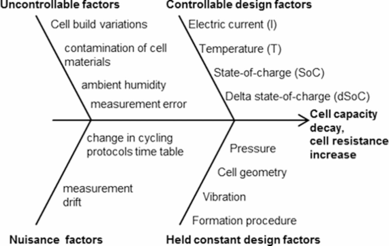
Figure 1. Fishbone-diagram of the identified causes effecting aging and the measurement thereof in lithium ion cells. The controllable design factors are researched in this paper, while all others contribute to the conduction boundary conditions of the experiment.
The study was conducted in order to demonstrate a method for statistically profound testing of lithium ion cells and shows the advantages statistical experimental design and analysis could provide for experimental cell development as well as estimation of cell survival times under certain loads. The method can certainly be applied to other types of energy storage devices also, but for of cost reasons was conducted using non-automotive, lab-size, non-series produced lithium ion cells. Stepping up to full-size cells will follow in a future study, since equipment is much more cost intense.
The basis of the design-of-experiment will be laid out in the experimental section. The measurement results of the conducted cell tests, and the statistical representation thereof, will be presented in the results section in detail. Finally the analysis of the statistical data will be discussed and the findings are pointed out in the discussion section.
Experimental
The study was conceived as large-scale aging experiment, therefore more than 150 cells were subjected to aging conditioning. Apart from planning how to distribute the sample points into the possible operating space of the cells, also the restrictions of the cycling equipment had to be taken into consideration.
The cells
Pouch cells of two different chemistries were studied: 99 cells which featured iron-phosphate cathodes and graphite anodes (further referred to as LFP cells) and 78 cells which featured nickel-aluminum-cobalt-oxide cathodes and graphite anodes also (further referred to as NCA cells). For reasons of energy consumption and safety of the experiment, a small cell size was selected for the cells. The cells showed initial capacities of 50 mAh (LFP) and 60 mAh (NCA) and consist of three square electrode sheets of the sequence anode (single layered) – cathode (double layered) – anode (single layered). During the whole experiment the cells were pressurized by using plastic clamps sitting on the outside of the pouch foil, in analogy to the straps commonly used in automotive applications, to hold the electrodes firmly in place. A common carbonate electrolyte (EC/EMC) and PP separator was used. The cells were especially designed and built for this experiment, using base electrode materials from Südchemie AG and cell building know-how from our project partner GAIA Akkumulatorenwerke GmbH.
Design-of-Experimental
Parallel to building cells, a Design-of-Experiment (DoE) was conducted. The DoE is a procedure which helps to plan and conduct an experiment such as to obtain statistically valid and objective conclusions.28 It consists of 5 steps, of which the first four will be explained in this subsection, for the last step see the explanations in sections Results and Discussion.
Statement of Experimental Target
The first step is an accurate statement of the experimental target. In this study, the aim was to determine the optimal settings of the key exterior influence factors on the target values "cell capacity decrease" and "impedance increase".11 The influence factors will be tested such as to find the optimum settings to prolong the time until the end-of-life criterion for one of the target values is reached. Taking into account the limited availability of cycling test equipment (max. 96 channels in parallel), only four exteriorly applicable parameters, were chosen for a given cell chemistry and geometry. The four factors are current, temperature, state-of-charge (SoC) and delta-SoC. The end-of-life criterion (EoLc) was formulated according to,29 as being a certain percentage of capacity retention as compared to the initial measurement. The limit was set to 60% remaining capacity for reasons of testing more than just the commonly required range of 80%. For the impedance increase a limiting percentage of 300% was chosen. Both values had to be measured always at the same temperature, which was found especially important for the impedance.
Screening and Test Plan Conception
The second step of the DoE procedure is the screening of the tested cells as well as the conception of the full factorial test plan. Screening means defining the range limits of the settings of the external influence factors (i.e. −15, 20, 50°C are settings for the factor "temperature") and testing of these limits regarding the cells' sensitivity in voltage response to setting combinations (i.e. are high c-rates at low temperatures possible?). The screening was mainly done by literature research, where many single-factorial variation experiments are on display.12,15,16,18,30 The fishbone-diagram in Fig. 1 was created out of the testing constraints and the results found in literature, wherein the "controllable design factors" are the influence factors to be actively varied in the test plan. From the number and assumed influences of "uncontrollable factors" the number of repetitions of each test point was determined to be at least three times, in order to obtain statistically valid results. On the bottom side of the effect arrow in Fig. 1 the factors are listed, which require special attention during the planning phase. It must be ensured that the "held-constant factors" are truly constant for the whole duration of the experiment, whereas the "nuisance factors" are points where very accurate calibration or additional measurement devices are supplied.
The four influence factors for this experiment are the temperature, the current (I, always given in c-rate), the average state-of-charge (SoC) and the amplitude or delta state-of-charge (dSoC). The temperature is given in degrees Celsius [°C], the range limits were set to −15°C and 70°C. For the current (expressed as c-rate) the generally accepted definition was applied, that the "c-rate is the current which corresponds to the cell capacity".22 The range of test for the c-rate is 0C (pure calendar aging) to 5C for charge as well as discharge. The average SoC is given in a range of [0...1]. The test will not exploit the full SoC range but will stay within 0.1 and 0.9, because it is not expected that a real-life application relies on the outer limits of the cell operation window. The dSoC is the SoC swing which is run through by a single constant-current pulse, which means that the SoC of the cell oscillates around the required average SoC by half of the dSoC value. The range limits of the dSoC will be 0 (calendar aging) to 0.8.
The full-factorial test plan is constructed out of each combination of the controllable factors in each of its factor levels. Factor levels are the numeric values in which the influence factor range is discretized, meaning for example the current factor range is 0 to 5 C, in which the levels are for example 0, 0.5, 1, 2 or 5 C. When considering the four identified controllable factors with five setting levels each, the full test plan has 45 = 1024 possible sample points and should be repeated at least 3 times in each point to eliminate the risk of testing an outlier with >90% confidentiality.
If the factor levels are chosen each within a physically possible range, the interaction with other factors' levels can be limited by the cell physics or the measurement equipment accuracy. The range of each factor, as well as the interaction limits found in literature, are marked as full (LFP) and dotted (NCA) lines in Fig. 2. In this figure the influence factors are given in columns and rows, so each plot shows the test space spanned by the two influence factors marked on the outside of the corresponding column and row.
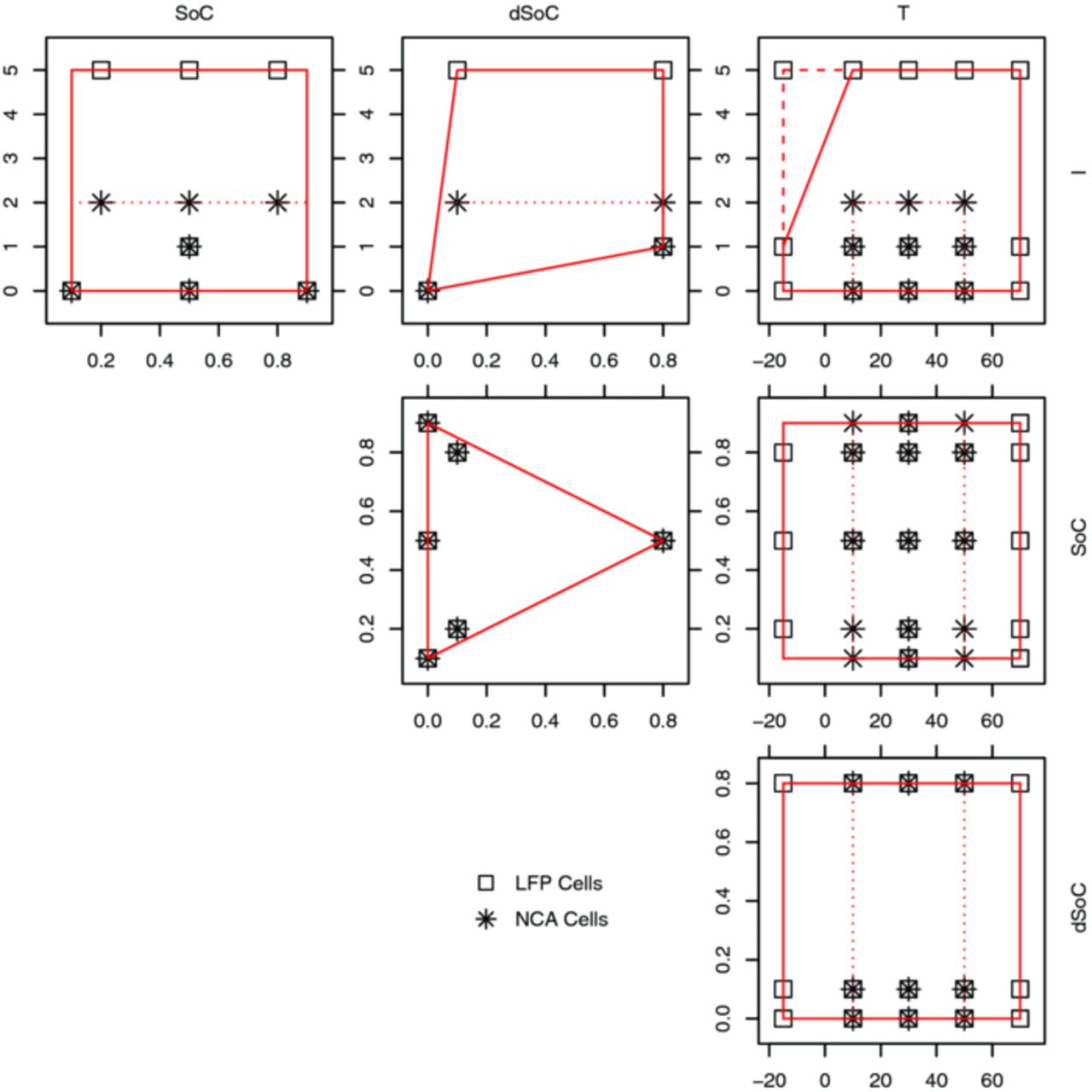
Figure 2. The design space of the experiment displayed in binary combinations of the influence factors, far side labels are valid for the whole column / row. Boundaries are displayed as full (LFP) and dotted (NCA) lines, test load points as squares (LFP) and stars (NCA). T in °C, I in h−1 (c-rate), SoC and dSoC in [0..1].
While considering imposable test limits, it is important to keep the test space convex,27 because after cutting away all the restricted spaces from the rectangular test space, a space must remain in which any two points can be connected by a straight line without crossing a limit or range border. Four such physically necessary limits were identified:
The first limit is the combination of dSoC with SoC, giving values larger than the SoC range, when added 1. The limit leads to the triangle shaped test space in the SoC vs. dSoC plot of Fig. 2 (center plot).
![Equation ([1])](https://content.cld.iop.org/journals/1945-7111/160/8/A1039/revision1/jes_160_8_A1039eqn1.jpg)
Second, the interaction of low temperatures and high currents was formulated as a limit, since cell cycling in this area could not be maintained within the operating voltage window. The current is empirically limited to 1C at −15°C, from 10°C upwards the full 5C is available 2 and top right plot in Fig. 2).
![Equation ([2])](https://content.cld.iop.org/journals/1945-7111/160/8/A1039/revision1/jes_160_8_A1039eqn2.jpg)
In 2 the temperature (T) is given in degrees Celsius [°C] and the current (I) in c-rate [h−1]. These numeric values depend strongly on cell micro and macro geometry as well as cell chemistry. Therefore this limit is not generally applicable with these values, contrary to the first limit.
The third and fourth limits concern the dSoC and current interaction (top center plot in Fig. 2). Both limits counteract the problem, that at zero current (I = 0) the dSoC is also always zero (and vice versa). When approaching this point with very small currents and/or very small dSoCs, the cycling equipment's accuracy will be the limiting factor. The limits were defined to not restrict the space more than up to the next factor level in current direction (1C) and in dSoC direction (0.1).
![Equation ([3])](https://content.cld.iop.org/journals/1945-7111/160/8/A1039/revision1/jes_160_8_A1039eqn3.jpg)
![Equation ([4])](https://content.cld.iop.org/journals/1945-7111/160/8/A1039/revision1/jes_160_8_A1039eqn4.jpg)
Since both limits are dependent of the cell chemistry and cycling equipment accuracy used, they are not applicable with exactly these values to every experiment, but the formulas are generally valid.
For the full-factorial test plan, the limits reduce the 1024 possible sample points by 230 not feasible points. So summing up for the cell count of the full-factorial experiment, a total of 3 * (45 - 230) = 2382 cells in 794 different sample points should be tested.
Test Plan Reduction
In the third step of the DoE process, the full factorial test plan is reduced, by using a modular algorithm for the design of large scale D-optimal experiments. The procedure and its implementation is thoroughly explained by Haselgruber in27 and used unaltered. The reduction is based on a criterion describing the usefulness of a single experimental point for the parameterization of an expected model for the target parameters. The score for the usefulness is called D-optimality of a design plan in statistical terms.
The algorithm selects a set of points in the corners of the test space as well as some points randomly distributed within the space. In each following optimization step it takes another random point out of the full factorial test plan, exchanges it with one point of, or adds it to, the initially selected points and calculates the change in D-optimality.28 If the D-optimality increases, the changes are kept and another point is exchanged. The optimization is finished if no more increase in D-optimality can be found. Such a coded test point matrix is displayed in,26 Table 2 for a visual reference.
After the screening process, it was assumed that a second-order statistical model would be the best way to express the expectations,31 without constraining the experiment too much. The target values (capacity decrease and impedance increase) are either linear or quadratic functions of a single factor or linearly dependent of the multiplication of two influence factors. The model was defined such as to incorporate offsetting the center of a quadratic term into the experimental range, an example of this model for capacity decrease is shown in 5.
![Equation ([5])](https://content.cld.iop.org/journals/1945-7111/160/8/A1039/revision1/jes_160_8_A1039eqn5.jpg)
This model definition accounts for all effects found in literature at the time of setting up the experiment, describing the capacity decrease and impedance increase depending on the chosen external influence factors.7,9,30 Table I gives an overview of influence factor transformations, which can be deduced from literature7–9,11,16,30 and which were used as a basis for the target parameter model of the DoE.
Table I. Overview of the influence factors and their transformations, deduced from literature, as basis for the target parameter model. The variables x and y stand for any numeric values within the ranges of the influence factors and introduce an offset from zero for the changes of influencing behavior. Sqrt(I) ... square root of I.
| Influence Factor | |||
|---|---|---|---|
| Temperature | Current | State-of-Charge | Delta State-of-Charge |
| T | I | SoC | dSoC |
| T2 | Sqrt(I) | SoC2 | dSoC2 |
| (T - y) | I2 | (SoC - x) | |
| (T – y)2 | (SoC - x)2 | ||
The exact model formulation, meaning whether every influence factor transformation has enough significance to remain in the resulting model, as well as the values for ai are not known until the analysis of the experiment.
Using the algorithm of27 the test plan was successfully reduced to 46 sample points, now fitting to the restrictions of the equipment available (channel number). These points are indicated in Fig. 2 for LFP cells (boxes) and for NCA cells (stars).
The fourth step of the design-of-experiment procedure is the conduction of the experiment itself, which is explained in the following subsections. Step 5 is the data analysis, which is presented in the sections Results and Discussion.
Experimental time schedule
The experimental planning was conducted under the premise that the measurement data acquisition is intermittent. This was necessary, because the capacity of the cell cannot be measured during 10% dSoC swings. So an experimental time schedule was drawn up, pictured in Fig. 3.
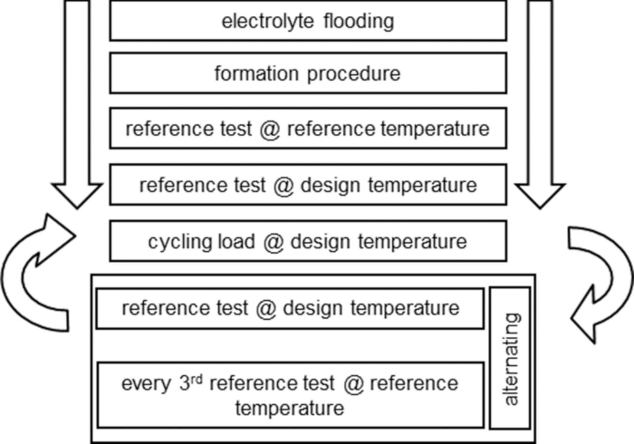
Figure 3. Flow chart showing the time order of the test execution. The first three blocks are performed within one week, the loop continues for the rest of the experimental time. The reference tests deliver the data points for statistical modeling.
The cells were built with the electrolyte in a squashable plastic bag, so they could be activated whenever the cell was required for the experiment. The first step after being connected to the cycling equipment is the formation procedure. After the initial cycles a reference test follows, which is described in detail in 2.4, conducted at reference temperature (30°C). Following this initial test, in order to make the cells comparable at start, the reference test procedure is applied a second time at the design-point temperature of the cell. The capacity measured in this second test forms the basis for the current rate to obtain the c-rate, at which the load cycling will be conducted. It was decided not to use the nominal c-rate for aging cycling, because otherwise the current density-dependent aging effects would be increasingly accentuated.
The cycling load as well as calendar aging (at a c-rate of 0 and a dSoC of 0), is periodically interrupted by reference tests, conducted at design temperature and at reference temperature. After reaching an end-of-life criterion in a reference test at reference temperature, the cell is taken out of the experimental setting.
Reference test procedure
The reference test procedure (RTP) was designed to be a measurement sequence which allows for a calculation of capacity decrease, impedance increase and their respective estimation errors as well as additional analysis data sets, such as differential capacity and differential voltage. It consists of an initial segment in which the cell is preconditioned to a full SoC (constant voltage charge at 3.8 V (LFP) / 4.2 V (NCA) until current < 0.05C). Then, a slow discharge at 0.2C is conducted for measuring the actual discharge capacity. This capacity is used as base for the following c-rate scan with 0.5, 1, 2, and 5 C (charge and discharge), each including constant voltage full charges in between (same as above). The third section is a galvanostatic intermittent pulse test, which has 5 pulse and rest periods at 0.5C in discharge and in charge direction (at SoC = 0.9, 0.7, 0.5, 0.3 and 0.1). This section is the base for calculation of the actual impedance32 of the cell. In the last part of the RTP a charge step followed by a controlled 50% discharge step set the cell to be ready to start a new load cycle. The RTP initialization and the load cycling restart are done by hand, because the new capacity has to be manually decreased in the control program of the cycling equipment.
Automation of data acquisition
The cycling equipment is an Arbin BT2000 with 96 channels ± 5 A in between 0 and 5 V with a measurement accuracy of ± 0.002 V and ± 40 uA in the used current range of ± 100 mA. Under the assumption that the measurement error follows a Gaussian distribution, the error for the capacity measurement is < 0.25% and the error for the impedance calculation is < 15%, for worst case settings with the given cells.
The status of aging is always calculated from a single RTP step, including the cell capacity, the cell impedance, the differential voltage and differential capacity:
- The cell capacity is calculated as being the value of the coulomb counter after the 0.2C discharge, which has been reset in end of the preconditioning charge preceding the discharge.
- The cell impedance is calculated from the pulse test of the RTP. For each current pulse of 0.5C a pulse impedance is calculated while switching on and switching off.32 The current rise time of the cycling equipment is <30 ms, so a time delta of 500 ms was chosen for the highest measurement frequency of voltage and current. Since the pulse test was done in charge and discharge direction, this equals to four calculated values per SoC level. A mean value for the impedance is calculated from all values at the same SoC level, since the expected difference between charge and discharge impedance is smaller than the measurement error. A linear regression is then applied to the mean values for the SoC levels to receive the median impedance for the cell.
- The differential voltage and differential capacity data is calculated from the same 0.2C discharge as the capacity. A constant current discharge is not the optimal base for this transformation, but a viable one according to.33
Results
In the following figures the experimental results for capacity decrease and impedance increase, the target values of the DoE, are displayed.
The plots are created with the lattice toolbox of "R", an open-source statistics program.34 The lattice-subplots all share their axes with the adjacent plots and throughout one figure. All axes have the same ranges within one figure. The x-axes are assigned the experimental time. The experimental time has been normalized to the longest lasting cell of each chemistry, because of the differences in endurance and the space available for tick marks. For LFP the normalized time range [0...1] is equal to 26 months, for NCA the normalized time range covers 18 months. Each subplot features a head panel showing the code for the displayed sample point. It consists of the four chosen influence values in the order temperature, c-rate, state-of-charge (SoC) and delta SoC (dSoC).
All cells which were run at one sample point are marked by dashed gray lines and the median value per time interval is shown in black. The red line is the cell in this sample point which is closest to the calculated median in most of the time steps. For further analysis and calculations all measurements of this cell are considered the realizations of the displayed target value per time interval, the other cells are considered repetitions and supply the variance values per time interval. For simplified comparison of the cells all measurements have been normalized to the first measurement after formation.
Capacity decrease
The experimental results for the capacity decrease are shown in Fig. 4 (LFP cells) and in Fig. 5 (NCA cells). There is a strong dependency of the capacity decrease on the test temperature for both chemistries. Although the test space for the two chemistries was slightly different (range limits for LFP cells: −15°C to 70°C, for NCA: 10°C to 50°C), the tests at 10°C were the ones resulting in the longest cell life time for both chemistries. For the LFP cells it is remarkable that cells being cycled at 1C do not age much faster than calendar aged cells, whereas cells cycled at 5C age significantly faster. For the NCA cells any cycling load ages the cells faster than calendar aging samples. For these cells the influence of the dSoC is stronger than the c-rate influence. These effects and additional, not directly visible effects of the other influence factors on the two cell chemistries will be highlighted during model built.
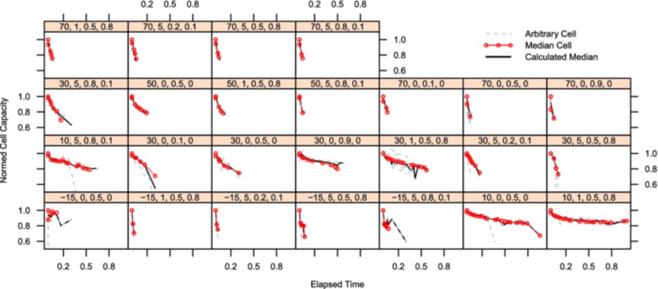
Figure 4. Each lattice box shows the normed cell capacity of all repeats of LFP cells running in a single test point on the y-axis over normalized experimental time on the x-axis. The test point is indicated by the number sequence in the bar above each chart in the following order: temperature [°C], current (as c-rate [h−1]), SoC, dSoC (both in [0..1]).
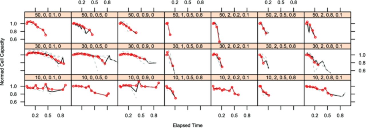
Figure 5. Each lattice box shows the normed cell capacity of all repeats of NCA cells running in a single test point on the y-axis over normalized experimental time on the x-axis. The test point is indicated by the number sequence in the bar above each chart in the following order: temperature [°C], current (as c-rate [h−1]), SoC, dSoC (both in [0..1]).
Impedance increase
The experimental results for the impedance increase are shown in Fig. 6 (LFP cells) and in Fig. 7 (NCA cells). The plots are structured the same way and show the data the same way the capacity decay plots do. The impedance and the time are again normalized to the initial measurement respectively the longest cell endurance.
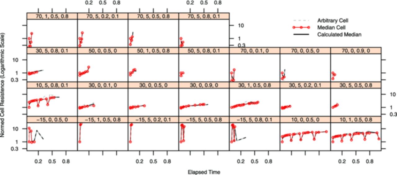
Figure 6. Each lattice box shows the normed cell impedance of all repeats of LFP cells running in a single test point on the y-axis over normalized experimental time on the x-axis. The test point is indicated by the number sequence in the bar above each chart in the following order: temperature [°C], current (as c-rate [h−1]), SoC, dSoC (both in [0..1]).
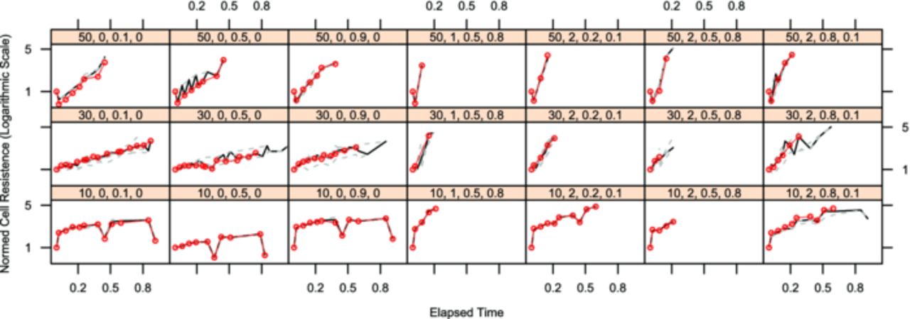
Figure 7. Each lattice box shows the normed cell impedance of all repeats of NCA cells running in a single test point on the y-axis over normalized experimental time on the x-axis. The test point is indicated by the number sequence in the bar above each chart in the following order: temperature [°C], current (as c-rate [h−1]), SoC, dSoC (both in [0..1]).
The impedance ticks on the y-axes are in logarithmic scales, due to the fact that the impedance is depending rather strongly on temperature. When temperatures below 10°C are applied to new cells, the impedance rises approximately 2.5 times per decade Celsius. Rising temperatures above 30°C do not affect the new cells as strongly, an impedance decrease of a factor of about 1.5 times per decade Celsius is observed. For aged LFP and NCA cells alike, these dependencies become less significant. Influences of factors other than temperature are not directly visible within the impedance data.
Differential capacity
Thompson33 and more recently Dubarry21 described how to read the changes of differential capacity over aging. Therefore, differential capacity plots were generated for the cells, as can be seen in Fig. 8 for a LFP cell (a and b) and a NCA cell (c and d). However, no other changes than a vanishing peak (upmost plot of b) to the right) for LFP and a shift to lower potentials for NCA could be observed. As both of these features are well visible in the discharge curves already, the peak shift data from differential capacity is not included in statistical analysis.
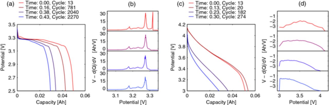
Figure 8. Comparison of the aging behavior of slow discharge voltage profiles and their respective differential capacity plots for LFP and NCA cells. a) LFP 0.2C discharge voltage versus capacity showing a rather constant behavior; b) LFP differential capacity, showing a vanishing peak but no shift of peaks; c) NCA 0.2C discharge voltage versus capacity showing a rather strong flattening; d) NCA differential capacity showing a clear shift of the capacity to lower voltages.
Statistical modeling
The fifth and last step in the DoE process (section 2.2) is modeling and analysis. There is a wide selection of statistical model methods available, which can be applied to the generated experimental data. Yet for the analysis of the DoE, the model which has been used for calculating the optimized design plan will be used for modeling. The basic model type is already shown in 5 and is a linear statistical model.
A linear model is not a time-dependent modeling method reproducing the data as seen in Figs. 4–7. The actually modeled data is represented by a single point in time per cell measurement. For the presented models this time is defined as the time needed for the cell to reach the end-of-life criterion for the modeled target value (see also Fig. 9).
![Equation ([6])](https://content.cld.iop.org/journals/1945-7111/160/8/A1039/revision1/jes_160_8_A1039eqn6.jpg)
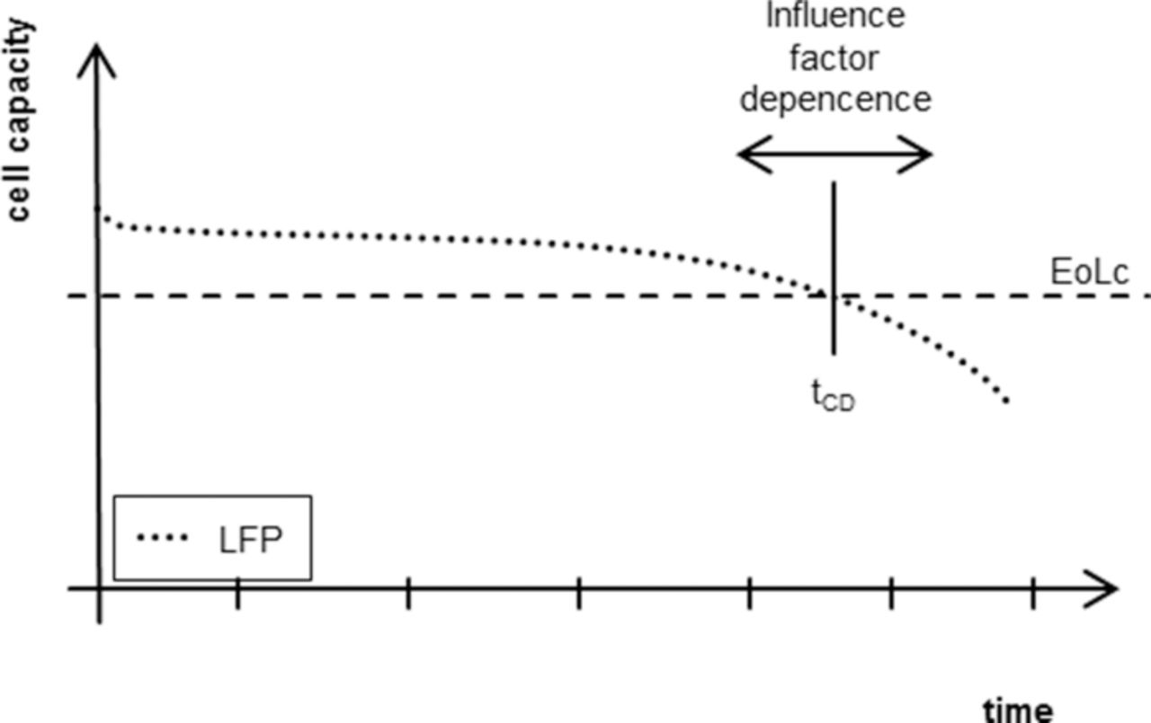
Figure 9. The presented linear statistical models of the cell aging only model the influence of the factors on the time until the intersection of the aging curve (ex. capacity decrease) with the end of life criterion and not the exact path behavior.
Each of the two target values, capacity decrease and impedance increase, will be treated in a separate model. Additionally separate models per chemistry were fitted. So a total of four parameter sets are presented in Table II (capacity decrease) and Table III (impedance increase).
Table II. Model parameters ai, their standard deviations and the resulting significance of the term for the LFP and NCA capacity decrease model. Empty rows indicate that this factor was insignificant for the respective model. An example for the construction of the model is given in 7.
| LFP | NCA | |||||
|---|---|---|---|---|---|---|
| Term Name | Parameter Estimate | Standard Deviation | Significance | Parameter Estimate | Standard Deviation | Significance |
| Intercept | 6,391·100 | 3,350·10−1 | *** | 8,9·100 | 1,127·10−1 | *** |
| T | 4,042·10−2 | 4,438·10−3 | *** | - | - | - |
| T2 | - | - | - | −4,488·10−4 | 6,854·10−5 | *** |
| (T-15)2 | −1,326·10−3 | 1,04·10−4 | *** | - | - | - |
| T * I | - | - | - | 1,994·10−2 | 5,119·10−3 | *** |
| I | - | - | - | −1,29·100 | 1,979·10−1 | *** |
| I * SoC | −7,513·10−1 | 2,131·10−1 | *** | - | - | - |
| SoC | 1,689·100 | 5,384·10−1 | ** | - | - | - |
| dSoC2 | −9,737·10−2 | 2,697·10−1 | - | - | - | |
| SoC * | - | - | - | |||
| dSoC | −2,305·100 | 3,044·10−1 | *** | |||
Table III. Model parameters ai, their standard deviations and the resulting significance of the term for the LFP and NCA impedance increase model. Empty rows indicate that this factor was insignificant for the respective model. An example for the construction of the model is given in 8.
| LFP | NCA | |||||
|---|---|---|---|---|---|---|
| Term Name | Parameter Estimate | Standard Deviation | Significance | Parameter Estimate | Standard Deviation | Significance |
| Intercept | 7,084·103 | 3,295·102 | *** | 3,799·103 | 9,812·102 | *** |
| (T-15)2 | −5,193·100 | 5,826·10−1 | *** | - | - | - |
| (T-15)4 | 1,361·10−3 | 2,091·10−4 | *** | - | - | - |
| T | - | - | - | 2,076·102 | 6,819·101 | ** |
| T2 | - | - | - | −3,857·100 | 1,034·100 | *** |
| dSoC | −4,325·103 | 2,556·103 | . | −1,402·103 | 8,015·102 | . |
| dSoC2 | 5,546·103 | 2,842·103 | . | - | - | - |
| dSoC * I | −1,627·103 | 5,701·102 | ** | - | - | - |
| I | - | - | - | −6,206·103 | 1,273·103 | *** |
| I2 | - | - | - | 2,816·103 | 5,877·102 | *** |
| SoC·*·I | - | - | - | −2,184·103 | 7,616·102 | ** |
The tables show three columns of values for each of the parameter sets. The values in the first columns are the estimates for the parameters of the model, received by least-square fitting. These estimates and the influence factor combinations for each term (found in the leftmost index column) form the model formula. For an increased accordance of the capacity decrease to a linear model (Fig. 9), the target variable tCD was transformed to a logarithmic scale. This step was not necessary for the target variable of the impedance increase tII. As examples, the final model formulations of the capacity decrease and impedance increase models for LFP from Tables II & III are presented in 7 and 8.
![Equation ([7])](https://content.cld.iop.org/journals/1945-7111/160/8/A1039/revision1/jes_160_8_A1039eqn7.jpg)
![Equation ([8])](https://content.cld.iop.org/journals/1945-7111/160/8/A1039/revision1/jes_160_8_A1039eqn8.jpg)
The center column displays the quadratic standard error for each estimated value coming from the least squares estimation. This value helps in deciding if a model term and the estimate are reliable and useful parameters or not, which is then displayed in the third column. Significance is given by a star rating, as common in many statistics tools such as R, more stars mean better reliability of the estimation (for more information see the R online help manual34), the formula for calculating significance is displayed in 9. The hypothesis, which the p-test is testing against, is that the estimate is actually zero. If true, the term is insignificant for the data description model.
![Equation ([9])](https://content.cld.iop.org/journals/1945-7111/160/8/A1039/revision1/jes_160_8_A1039eqn9.jpg)
A rating of three stars means that the term is highly significant and should not be left unconsidered. Two and one star are a little less significant. A point means the user should decide based on his knowledge of the subject, if the term should be considered.
Not all the influence factor combinations mentioned possible in Table I can actually be found in Tables II and III, because the models have already been reduced by all insignificant combinations. This process starts with the graphical interpretation of a factor plot as seen in Fig. 10. It exemplarily displays one model target parameter (tCD) for the LFP cells in dependence of a single influence factor (x-axis) averaged over all combinations with the remaining three factors. This plot tells which of the influence factor terms will very likely be significant and need to be taken into account for the model. In the upper right hand plot of Fig. 10 the maximum at 10°C visualizes the need for a center value different from zero for the quadratic temperature influence term for LFP, since this term would otherwise always be centered at zero. Alike, plots exist for the first order interactions, as shown in Fig. 11 for the data of the LFP cells. It tells which interactions are to be retained in the model for tCD of LFP. In the rightmost graph a weak interaction of SoC and dSoC is indicated, which showed to be insignificant during model reduction. It is a repeated process of taking a model, starting out with all possibilities of Table I, and reducing the insignificant ones, then refitting the model. This process is repeated three times per target value and chemistry, always reducing the model by all parameters which had no or very low significance (< 10% in the p-test). The improvement in model quality during the process is monitored in the four model graphs (Residual vs. Scaled, QQ-Normal, Scale Location and Leverage, see 28) given by the plot model command in R and the decreasing AIC value (Akaike Information Criterion).31,35 These steps are not explained in detail here, but can be found in the R help files.34 The models stayed very much the same across the chemistries during the first repetition, but differences arose in the following iterations. All models acquired good model quality during the fitting process.
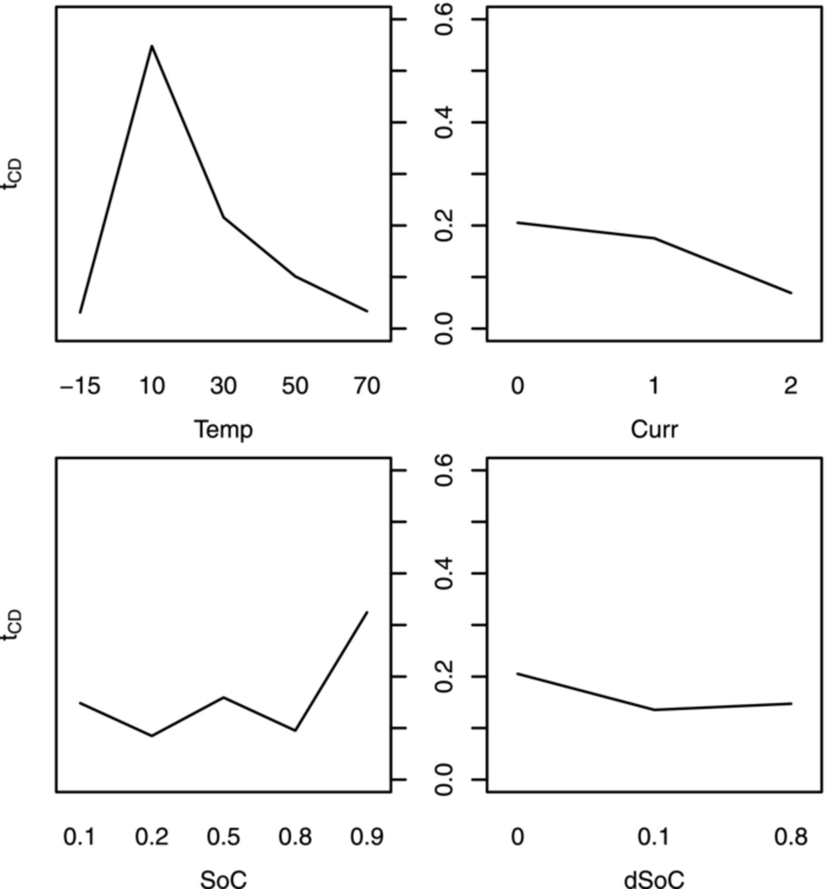
Figure 10. Exemplary influence factor plot for the model deduction (LFP cells). An average of the target variable (y-axis of each plot) over all cell data containing a single setting level of an influence factor (x-axis) is shown per factor. This plot identifies center offsets, as can be seen in the left upper plot for the temperature. The according offset was set to a center of 15°C. Temperature (Temp) [°C], current (Curr, as c-rate [h−1]), SoC, dSoC (both in [0..1]).
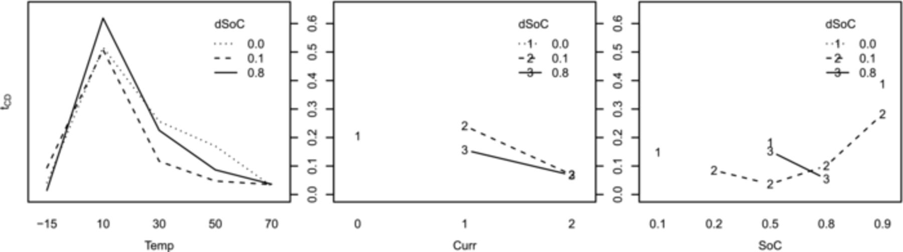
Figure 11. Exemplary factor interaction plot for the model deduction (LFP cells). An average of the target variable (y-axis) is displayed per factor setting, as indicated in the legend, over the factor settings of the y-axis factor. A weak interaction of SoC and dSoC can be seen in the rightmost subplot. Temperature (Temp) [°C], current (Curr, as c-rate [h−1]), SoC, dSoC (both in [0..1]).
Discussion
Measurement results
When reviewing the aging measurements of the capacity measurements it is notable that the cells do have some variance in their response to the influence factor combinations in a lot of the sample points. Since all cells were hand-made and the cells are only covered by a single layer of pouch bag foil, this was expectable to happen (Fig. 1). A countermeasure taken was to steady the active material parts by plastic clamps before the start of the experiment. As a second measure, a larger number of cells than required by the DoE plan was tested in some sample points to characterize the real-cell variance well. These sample points are enlarged in Fig. 12 for LFP (left) and NCA (right). The sample point selected was 30°C, 1C, 50% SoC and 80% dSoC for reasons of space for additional cells and channels being available in the 30°C test chamber and the electric load being a medium test point except for dSoC. The resulting variance in this test point is rather large, but it is also visible that most of the cells had the same characteristic path in their capacity decay. Among cells of the same chemistry the path is very common, but not shared by the other chemistry. LFP containing cells seem to age in a double dip behavior with an elongated plateau in between, while NCA cells experience a capacity rise in the first stage of their life and decrease their capacity continually down without plateaus later on. For both chemistries the different stages of aging (Fig. 13) are characteristic. Both cell types use the same anode, which indicates that at least the difference in aging behavior within LFP stage I & II versus NCA stage I can be attributed to cathode causes. The length in time of single stages is dependent on the influence factors, but the strength of influence factors is different between the stages in each sample point.
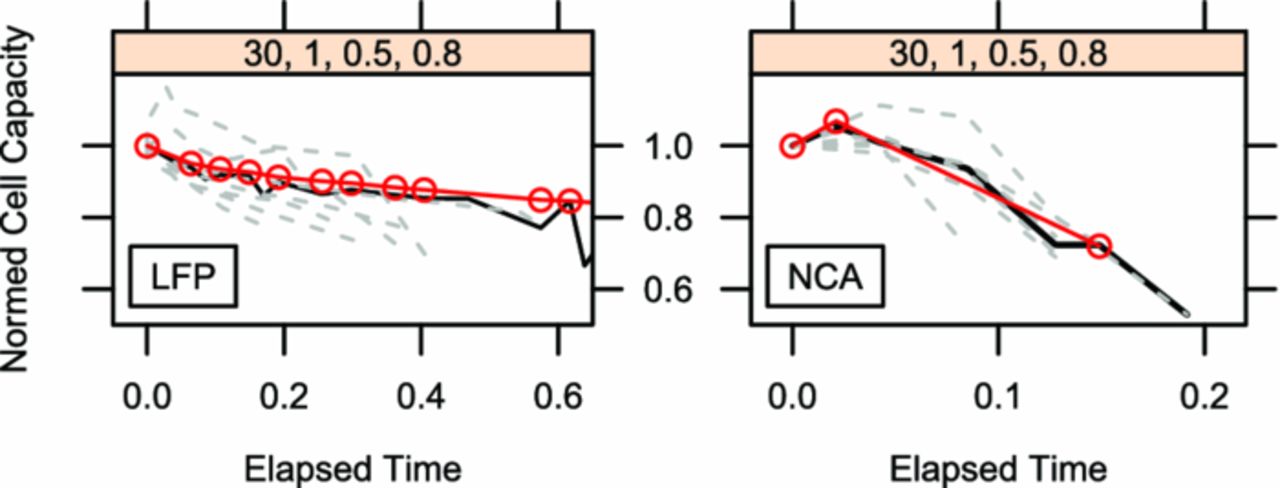
Figure 12. Zoom into two of the plot lattices of Fig. 4 (left) and Fig 5 (right). It shows the normed cell capacity of all repeats (dashed light) of the test point with the most cell repeats per chemistry over the normed testing time. The variance in numeric value is rather large, but the path behavior is similar per chemistry. The mean value is indicated by a red line with circles, the median cell (the most representative cell) is indicated by a dark line.
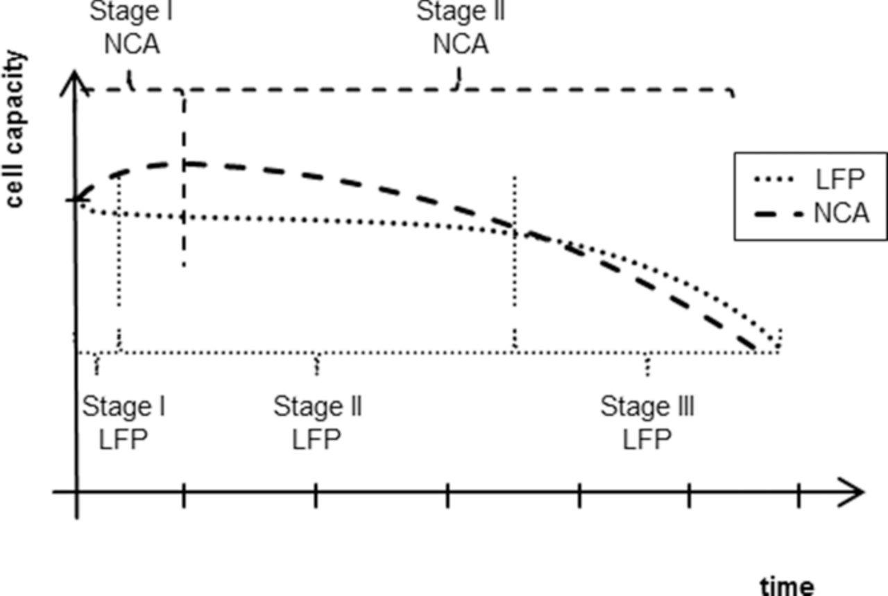
Figure 13. The deduced characteristic aging paths of the target parameter normed capacity for the two different lithium ion cell chemistries. Indicated are the stages in which the behavior can be split. For LFP three stages were found: initial losses, stable plateau and fall off. For NCA only two stages were found: run-in and accelerating loss phase.
Additionally having a build variance, some of the cells showed electrolyte leaks at the electrode bushings. This was an effect which was not initially expected and no specific countermeasures were taken. During model fitting it showed that there was no significant alteration of the aging path for both chemistries due to these leaks presumably due to an electrolyte excess, though it did accelerate the capacity decrease of heavily affected cells. The data of those cells was taken out of the data base before the statistical analysis.
The aging measurements of the impedance were expected to show visibly more variance than capacity measurements due to the measurement accuracy of just less than 15%. This expectation cannot be directly supported by the data presented in Figs. 6 & 7, because the measurements show a more articulate dependence on the actual temperature than on the aging influence factors or the measurement accuracy. The expectation of a characteristic shape of impedance increase has therefore to be reduced to a linear increase, fitting very well to the linear modeling. Still this linear increase has a slope depending significantly on all influence factors, not only temperature. For future experiments all reference tests should be at reference temperature to get less disturbed results. The found impedance increase ranges between factor 2 and 4,5 during the lifetime of the cell. At low temperatures there exist values exceeding the EoLc (factor 3) which was set for the impedance, but only measurements at reference temperature (30°C) were taken for the activation of EoLc.
The results from the impedance increase measurements are especially interesting for the design and sizing of cooling systems and power inverters. It implies that a system able to cope with all temperature levels of a new cell, can handle an aged cell with very little additional capacities needed.
Statistical modeling
Single factor variation experiments are rather easy to analyze, since one can tell the difference in cell aging by looking at the graphs of the different sample points. In this study a total of 46 sample points are tested and the factor level combinations are not linearly varied, so one has a hard time to see differences in sample points intuitively. Hence, a discussion of the model parameters of the presented statistical models is needed. In these parameter sets one can see the influence strength, the differences between sample points and chemistries in a more compact way. Fig. 14 and Fig. 15 show the capacity decrease model and the impedance increase model respectively in a telling way. These plots show within the top right triangle the LFP model and in the lower left part the NCA model. In both halves of the plot are box graphs bounded by the limits of the design space as introduced in Fig. 2. The axes of the design spaces are given in the main diagonal, the labeled contour lines within the design space boxes are the model responses (the survival time until EoLc). So a higher contour label encircles an area of an exponentially longer survival area. Each box graph gives the variation in survival deviating from the standard point of 30°C, a current of 1C and SoC as well as dSoC equal 0.5. If not varied for the graph, these values rest constant.
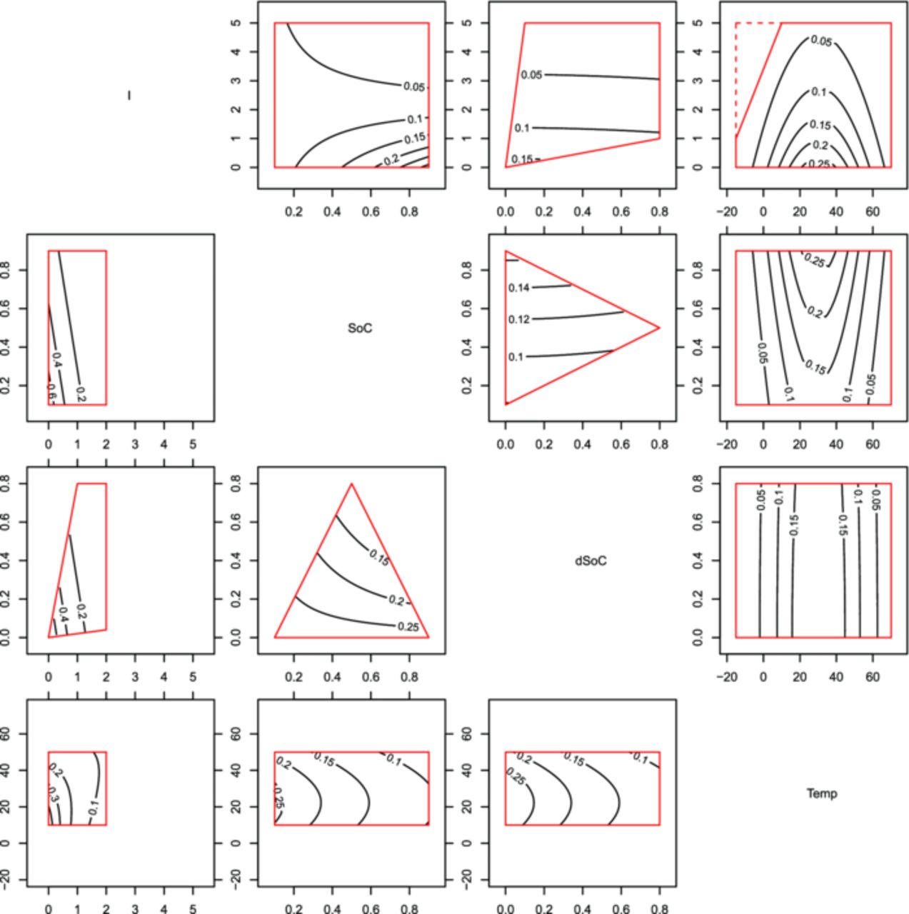
Figure 14. Normalized survival times, as predicted by the capacity decrease model plotted as isocontours within the experimental limits. Above the diagonal is the LFP, below is the NCA data model. Since one plot only shows the variation of two influence factors, the others were fixed to the settings completing the load point of Temp = 30°C, I = 1 h−1, SoC = 0.5, dSoC = 0.5.
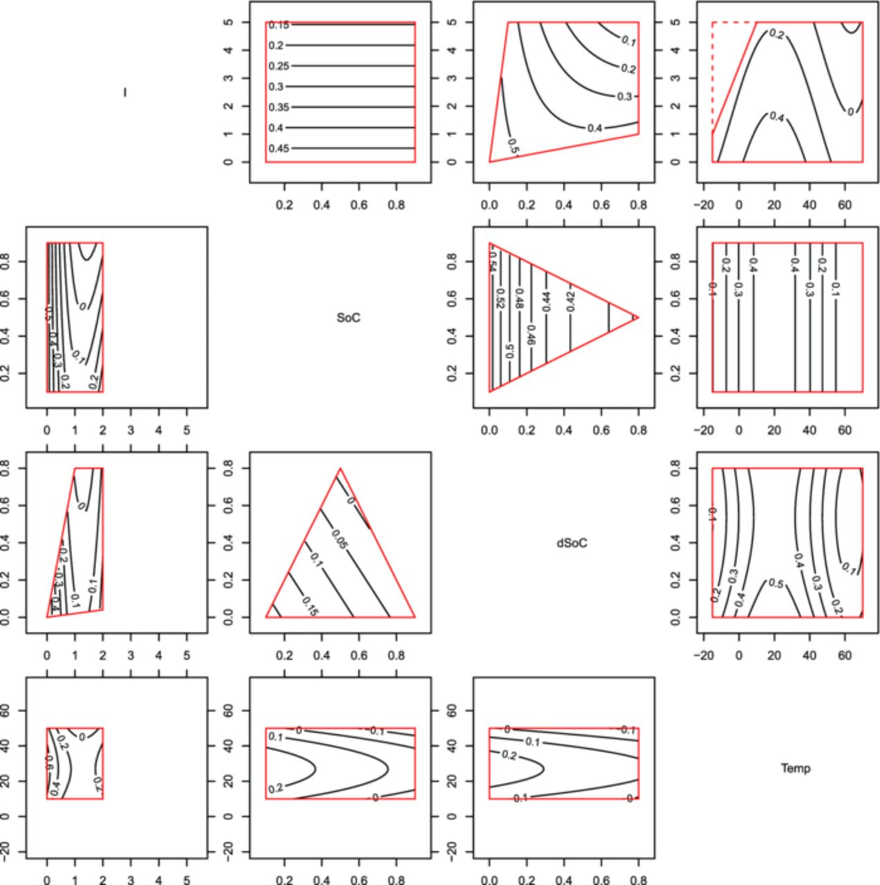
Figure 15. Normalized survival times, as predicted by the impedance increase model plotted as isocontours within the experimental limits. Above the diagonal is the LFP, below is the NCA data model. Since one plot only shows the variation of two influence factors, the others were fixed to the settings completing the load point of Temp = 30°C, I = 1 h−1, SoC = 0.5, dSoC = 0.5.
As for the influence parameters in both models it is remarkable – although in different powers and with different center values – how basic influence factor combinations are reduced per model and chemistry to a maximum of three out of four parameters tested. A stronger reduction is present in the interactions, which were reduced from 6 possible to about 3 significant interactions per chemistry only.
Temperature
There were five measurement settings in temperature for LFP cells, covering a range of −15°C to 70°C, and only three for NCA cells, ranging from 10°C to 50°C. The measurements suggest a maximum survival time at around 10°C to 15°C (Fig. 10), which was modeled by offsetting the temperature influence to +15°C. The effects leading to the maximum in survival time are suggested by literature8,36 also, underlined by the fact that the cells, which operated at low temperatures, showed lithium deposition on the anode upon visual inspection after experiment ending. The strength of the aging influence due to temperature as postulated from the measurements is schematically depicted in Fig. 16. The finding is that a cell operation temperature of around 10°C to 15°C would keep capacity decrease and the impedance increase low, although this temperature shows a higher power derating due to increased impedance compared to standard 30°C operation. So the compromise between life and operation conditions would be an operation in the window of 15°C to 20°C.
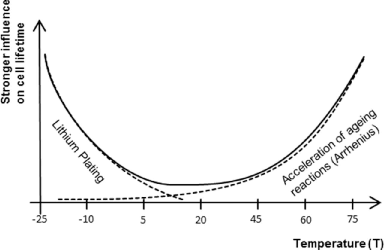
Figure 16. The aging influence of the temperature is a combination of different aging effects, producing a centered exponential influence on cell aging.
Current
All four models favor a smaller current for the reduction of aging effects. The lowest tested average current over aging was close to zero, meaning the cell was under calendar aging only, which also was the most favorable point. However, it is likely that the charging and discharging currents have different influences on the aging and will therefore be regarded as separate influence factors in future works.
dSoC
All four models favor smaller dSoCs for the reduction of aging effects. The lowest tested dSoC was equal to zero, meaning the cell was under calendar aging only, which also was the most favorable point.
The dSoC was found to especially enhance NCA aging when being high. SEM pictures, taken after disassembling aged cells, point toward a mechanism of particle destruction (Fig. 17).
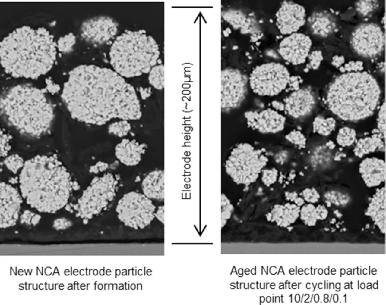
Figure 17. Detail of two REM pictures of a new (left) and an aged (right) NCA cathode. In the right picture the average particle size is smaller and more fragments are visible. The electrodes are shown in their whole thickness, the gray strip on the bottom is the aluminum current collector.
SoC
For the SoC very different results were found for the two chemistries. While for NCA cells low average SoCs were favorable for a low capacity decrease as well as impedance increase, the most favorable SoC for the LFP cells was found to be at higher SoC values for a low capacity decrease, and a non-issue for the impedance increase. A mechanistic explanation for this could be that the issue observed is a matter of mechanical cell balancing. LFP is changing its particle and consequently its electrode volume over SoC. This fact applies for graphite also and, if balancing is right, the ratio is about the same for both electrodes. NCA is changing its volume less,37 so the volume expansion of the graphite electrode cannot be counter balanced by the NCA electrode. So a mechanically relaxed electrode stack state in NCA cells is the discharged state. For LFP cells it is the fully charged state, because the graphite has a higher volumetric capacity than LFP but not a comparably larger volume expansion. Other explanations could be electric contact loss in LFP and inner recrystallization in NCA particles.38
Interaction of SoC and dSoC
This interaction is strongest for the NCA cell's capacity decrease. In NCA cells a large dSoC causes heavy aging and if additionally the SoC is high, a high cell pressure (see SoC) could enhance the particle destruction effect (see dSoC). So the interaction accelerates the aging process when both factors are at high settings.
This interaction is not relevant for LFP cells.
Interaction of current and dSoC
LFP cells exhibited a medium strength interaction of current and dSoC for the impedance increase while having a strong weight on dSoC. This interaction shows that high currents for small dSoCs are not much worse than small currents for large dSoCs, which is an often found result for aging experiments of lithium ion cells (see various data sheets, e.g. in39), although not often tested for as real interaction.
This interaction is not relevant for NCA cells.
Interaction of current and SoC
For both chemistries alike, this interaction suggests low aging when large currents are applied to an empty cell and stronger aging when large currents are applied to a charged cell. Since both cells feature the same graphite anode, the interaction could be an effect coming from anode. In favor of this theory would be the known issue that high charging currents at high SoCs enhance the risk of plating.9,11 It is likely that the charging and discharging currents have different influences on the aging.
Looking at the LFP cells separately, this interaction and the single influence of SoC combined give the suggestion that the cell has a window around medium SoC, in which large currents and zero current (storage) are favorable. At high and low SoCs the survival time is decreasing. The current limitation at high SoC exceeds the positive effect of the high SoC at very extreme values only. So a compromise in cell operation is suggested in using only medium to high SoCs as operational range (e.g. 80–35%). Again, it is likely that the charging and discharging currents have different influences on the aging.
Interaction of temperature and current
This interaction has a positive sign for NCA cells, so it favors larger currents only at higher temperatures for the capacity decrease model. It is a rather strong term in the model. It can be interpreted that local heating due to high currents has less impact when temperatures are already high and the impedance is low. The interaction has no significance for LFP cells.
The remaining, not mentioned interactions of the four influence factors were either not or weakly observed in the results and are therefore not statistically supportable as results. Since this study covered two very different cell chemistries, one could postulate that their influence will be small for other lithium ion cell chemistries as well.
When setting up a new design-of-experiment with the herein discussed influence factors and their ranges, those interactions can likely be neglected. Doing so will distribute the load points during the calculation of the design plan in a different manner. Points, which only add information about one of the neglected interactions, will not be taken into the reduced design plan. Therefore the experiment will be more focused on better description of the model terms identified as important in this study.
The model results
The model not only provides a good overview of the experimental results, but also has a real value for someone trying to calculate the survival time a cell under a load profile. Any of the applications mentioned in the introduction demand loads which fit well within the test space and can therefore be safely evaluated with this model. Some current publications39,40 use models which only rely on single data sets of dSoC variation, which could profit very much by applying models like the one presented here.
When an expected profile is at hand, calculation of the average values for the four influence factors is needed. Taking those as input of the model it will return a survival time for the cells used in this experiment. Since the model can very quickly be evaluated for many different load profiles versus battery pack combinations, this can give a very good hint on how to tune the load or size of the pack in order to reach the desired lifetime. The model presented holds true for the cells tested and needs reparameterization every time a new cell is regarded. General trends on cell aging depending on the cell chemistry can, however, be derived.
Conclusions
In this study we presented the statistical method of design-of-experiment applied to aging of lithium ion cells of two different chemistries, giving a model of the influences and some hints on the basic causes of cell aging. The method proved easily applicable and the results open the doors to more focused further electrochemical research in analysis of aged cells. All important aspects, from design space limitations and design plan deduction to the modeling and analysis of the experiment were shown and described for easy application in future experiments. The results obtained from these experiments are statistically sound and can therefore be reproduced, unlike single cell, single-factor experiments.
Of the initially proposed four influence factors, all four pure factors were found to be significant to the aging performance of the two cell chemistries, even though it were three out of four per chemistry. Only five among the possible interactions proved to be statistically significant, again only three per chemistry. So knowing the electrochemical background of aging of a researched cells' chemistries one could now initially reduce the design plan by those interactions.
The model provides insight into the processes leading to a change in external cell behavior and can be applied for dimensioning and aging analysis of future lithium ion cell applications.
For a future work a study based on design-of-experiment on series produced cells with a longer life span will be conducted. Therefore, the found models will be used as basis for the design plan optimization. Furthermore, post-mortem analysis of the cells will be added in order to support the electrochemical interpretations made.
Acknowledgment
The authors acknowledge the financial support of the "COMET K2 - Competence Centers for Excellent Technologies Program" of the Austrian Federal Ministry for Transport, Innovation and Technology (BMVIT), the Austrian Federal Ministry of Economy, Family and Youth (BMWFJ), the Austrian Research Promotion Agency (FFG), the Province of Styria and the Styrian Business Promotion Agency (SFG).
We would furthermore like to express our thanks to our supporting industrial and scientific project partners, namely AVL List GmbH, GAIA Akkumulatorenwerke GmbH, Volkswagen AG, University of Münster and to Graz University of Technology.