


ABSTRACT
We present a detailed study of the close eclipsing binary BS Vulpeculae. Although it is relatively bright (V: 10.9–11.6 mag) and belongs to short-periodic variable stars (P = 0.48 days), it is rather neglected. To perform a thorough period analysis, we collected all available photometric observations that span the time interval of 1898–2010. Observations include archive photographic plate measurements and visually determined eclipse minima timings done in 1979–2003, which were later shown to be biased to accommodate the existing linear ephemeris. Applying our own direct period analysis we found a well-defined shortening of the orbital period of dP/dt = −6.70(17) × 10−11 = −2.11(6) ms yr−1, which implies a continual mass flow from the primary to the secondary component. Using the 2003 version of the Wilson–Van Hamme code, our new complete BV(IR)C light curves were analyzed and the physical parameters of the system were derived. We found that BS Vul is a near contact binary system with the primary component filling its critical Roche lobe. The luminosity enhancement on the left shoulder of the secondary minimum shown in the light curves can be explained as a result of a persistent hot spot on the secondary due to the mass transfer from the primary component to the secondary one and heating the facing hemisphere of the secondary component, which is consistent with our result of period analysis. With the period decrease, BS Vul will evolve toward the contact phase. It is another good observational example as predicted by the theory of thermal relaxation oscillations.
Export citation and abstract BibTeX RIS
1. INTRODUCTION
Near contact binaries (NCBs) have been defined by Shaw (1990) as a subclass of close binaries with both components filling or nearly filling their critical Roche lobes (RLs). They display strong tidal interaction and show β Lyrae type variations. According to the geometric definition of this subclass, NCBs actually comprise semidetached, marginal contact and marginally detached systems. As we know, once a component fills its critical RL, mass transfer will occur and manifests itself by the presence of a hot spot on the surface of the mass accepting component. Therefore, NCBs are good targets to study mass transfer in close binaries. In addition, with mass transfer NCBs could evolve into detached or semidetached contact binaries, so they are important targets which lie in the intermediate stage between these systems. NCB targets are relatively rare because this stage is a very short phase compared to the lifetime of close binaries (Zhu & Qian 2006; Zhu et al. 2009, 2010). In order to study these rare systems, we observed a group of NCBs including our present target BS Vul, which displays a slightly asymmetric β Lyrae type light curve.
The light variations of BS Vul (= GSC 01614−00702 = HD 344650 = BD+21 3850; α = 19h37m27s, δ = +21°55'50'', 2000.0) were revealed on photographic plates of the Sonneberg observatory survey by Hoffmeister (1928). Jacchia (1940) determined a light ephemeris based on Harvard plates made in the period 1898–1939. Grigorieva (1938) found BS Vul on 18 plates of the Moscow photographic survey done in 1898–1917. The first photometric observations were done by de Bernardi & Scaltriti (1979), who gave the light ephemeris for primary minima as 2, 443, 271.579 + 0.47597198 × E. Shaw (1994) included this star in his list of near contact binaries and gave the spectral type as F2, apparent magnitude mV = 11 mag with the depths of minima as 0.7 and 0.2 mag, respectively, and the distance of the system as 460 pc. Although BS Vul is a quite bright (V: 10.9–11.6 mag) system that has been known for many decades, it remains neglected.
In this paper, we present the detailed period analysis of BS Vul. Orbital period investigations are important in close binary studies because they can provide us with some information about the important physical processes occurring in close binaries, such as mass transfer, magnetic activity cycles, and the interaction with additional bodies, and give us a hint of the evolutionary stage of the binaries. For obtaining an accurate period and period changes, long-time-span data sets are needed. Thus, the earlier timings are important. However, most of these earlier timings are less precise, i.e., visual and photographic timings are sometimes not very reliable due to the inherent biases of the observers. So we collected all available original data of BS Vul and used our own direct period analysis method to obtain reliable results. We then used the WD code to analyze our high-precision light curves to derive the photometric solutions. Finally, we combined the period changes with the photometric solutions of BS Vul and discussed the geometric structure and evolutionary stage of this system.
2. OBSERVATIONAL DATA
New observations of BS Vul were carried out on 2009 October 19, 22, 25, and 26 (2568 measurements) and 2010 November 4, 7, 10, and 11 (3730 individual magnitudes) with the PI1024 BFT camera attached to the 85 cm telescope in Xinglong Station of the National Astronomical Observatory, China. A standard Johnson–Cousins–Bessel multicolor CCD photometric system built on the primary focus was used. The effective field of view was 16 5 × 165. GSC 01614−00892 (α = 19h37m20s, δ = +21°51'38'', 2000.0) and GSC 01614−00678 (α = 19h36m57s, δ = +21°52'17'', 2000.0) which are near the target, were chosen as comparison and check stars, respectively. We set the integration time for B, V, RC, IC filters as 10, 7, 6, 5 s, respectively. The aperture photometry package of IRAF was used to reduce the observed images. From the observations, the complete BV(IR)C CCD light curves of BS Vul were obtained (see the entire version of Table 1 in the online journal). The typical photometric error for any single measurement was ±0.016 mag.
Table 1. CCD Photometric Observations in BVIR Bandpasses for BS Vul Observed in 2009 and 2010
| HJD | Differential Mag |
|---|---|
| (d) | (mag) |
| B-band | |
| 2455123.941462 | −0.545 |
| 2455123.942481 | −0.541 |
| 2455123.943511 | −0.542 |
| 2455123.944529 | −0.541 |
| 2455123.945560 | −0.532 |
Only a portion of this table is shown here to demonstrate its form and content. Machine-readable and Virtual Observatory (VO) versions of the full table are available.
Download table as: Machine-readable (MRT)Virtual Observatory (VOT)Typeset image
However, these observations were made only recently. To improve the accuracy of the BS Vul period and study its expected changes we need a much longer time span. Traditionally, we could use the (O − C) diagram of minima timings. Nevertheless, after many years of experience with period determinations, we preferred the direct period analysis method which uses complete phase information of all available individual measurements (see, e.g., Mikulášek et al. 2011b, 2012) containing phase information. In order to obtain reliable results, it is better to collect as many individual observations/measurements as possible. In addition to the new observations, the following data sources were used for a detailed analysis of the orbital period.
- 1.Grigorieva (1938): 18 measurements on plates of the Moscow photographic survey with a scatter of 0.13 mag (JD 2 414 433.4–2 421 484.3).
- 2.Szafraniec (1962): 200 visual estimates of brightness made by S. Piotrowski in two time intervals (1935–1939 (155 estimates) and 1945–1946 (45 estimates)). The data sets are quite homogeneous since estimates were done by one experienced observer (scatter of estimates being 0.18 mag), and thus we can use them in our method of data processing even though these are only visual estimates. We only had to transform his "magnitudes" to standard ones by scaling them by a factor of 2.65.
- 3.De Bernardi & Scaltriti (1979): 626 measurements in V with a scatter of 0.04 mag made from JD 2,443,247.5 to 2,443,406.5 at the Astronomical Observatory at Torino, Italy using a 0.45 m reflector equipped with a photoelectric photometer with an uncooled photomultiplier EMI 9502.
- 4.ASAS-3 (Pojmański 1997): 217 CCD survey measurements between JD 2,452,735–2,455,110 in V with a scatter of 0.03 mag.
- 5.OMC INTEGRAL: Optical Monitoring Camera on board of the INTEGRAL satellite (for details see Mas-Hesse et al. 2004) made 517 measurements in the V band during the time interval of JD 2,452,761.6–2,454,215.2.
- 6.AAVSO archive, 301 CCD observations with scatter of 0.07 mag made by Gerald Samolyk, U.S.A. in the V band over three nights: 2,455,005.5, 2,455,146.5, and 2,455,380.5 (http://www.aavso.org).
- 7.There are also some original BS Vul data from the ROTSE and PI surveys; however, their quality is so poor that we decided not to use them.
3. PERIOD ANALYSIS
3.1. Direct Period Analysis without Using O − C Diagram
The basic version of our direct period analysis entails the modeling of observed orbitally modulated variations making use of suitable models containing the orbital period and its pertinent secular changes as free parameters. In the present study, we limit ourselves only to analysis of light changes.
The first step of our more or less phenomenological modeling is the finding of the appropriate model function, F(t), that correctly describes the variations observed in the light curve of BS Vul. We aimed to search for functions with as few free parameters as possible. Comparing shapes of BS Vul mean BVRI light curves during the last several decades we concluded that all of them are nearly symmetrical with deeper primary and shallower secondary minima centered on 0.0 and 0.5 phases.
The shapes of individual light curves of BS Vul were described by the depths of primary and secondary eclipses a1b, a2b in the b = {B, V, R, and I} photometric bands, as well as the mean magnitudes outside of eclipses for the jth observer  . Light changes caused by proximity effects can be simulated by a simple double-wave cosinusoid with a semi-amplitude a3 unique for all photometric bands. The shapes of light curves during both eclipses could be described by the unique parameter C, the widths of primary/secondary minima d1, d2. In total, we analyzed 14 light curves, containing 8177 individual measurements obtained in four different photometric bands by eight different observers.
A detailed inspection of the observed  light curves indicated that there was an additional persistent light contribution that occurred between phases 0.25 and 0.45. Using the WD code, we modeled this excess as a hot spot on the secondary star (see Section 4). This effect was approximated by the last term described by three free parameters a4, d4, φs.
The observed light curves were then approximated by the model

where φ1, φ2 are the phases and ϑ(t) is the time-dependent phase function. The operator "round" rounds the argument to the nearest integer, while "floor" rounds the argument to the nearest integer toward minus infinity. The phase function ϑ(t) (for details see, e.g., Mikulášek et al. 2008, 2011a) is the monotonically increasing function of time t of which the integer part is the epoch E and the fractional part is the common orbital phase φ with zero phase put at the center of primary minimum. The phase function ϑ(t) thus has its origin at the time of the epoch origin M0. Knowing the phase function we are able to determine the phase for any time. Wanting to solve the reverse task: to predict the moment of zero phase (primary minimum timing) for any epoch E, we need to find the inversion function of the phase function θ(ϑ).
The phase function ϑ(t) is bound with the instantaneous period P(t) by the relation

We found that the instantaneous orbital period P(t) of BS Vul is monotonically decreasing. Using Equation (3) and assuming the linear decrease of the period (Equation (4)) we can derive the exact expression for the phase function ϑ(t) and its inversion function θ(ϑ)


where P0 is the instantaneous period at the moment t = M0 and  is the time derivative of the period. Since the decrease in period
  is very small, the functions ϑ(t) and θ(ϑ) can be replaced with their Maclaurin series expansions as follows:
Since the last terms in Equations (7) and (8) do not exceed 1.2 × 10⁻⁹ and 3 × 10⁻¹⁰ days, respectively, for any of the used measurements, we can restrict ourselves to only two (Equation (7)) or three (Equation (8)) first terms of the expansion.
All free parameters including  were computed by a standard weighted nonlinear least-squares method (LSM) regression applied to all the observational material (see, e.g., Mikulášek et al. 2011a). Weights of individual measurements were inversely proportional to the squares of standard deviations σ of their subsets with respect to the chosen regression model (Equation (1); see also Table 2).
Table 2. Virtual Times of Primary Minima and (O − C) of BS Vul versus the New Ephemeris Derived from Measurements Used for Its Orbital Period Determination, Number of Observations, Scatter in mag, and the Source of Photometry
| HJDI − 2400000 |  |
Type | N | σ | Source |
|---|---|---|---|---|---|
| (mag) | |||||
| 17707.134(6) | −0.0075 | pg | 18 | 0.15 | Grigorieva (1938) |
| 28506.0026(17) | 0.0051 | vis | 155 | 0.16 | Szafraniec (1962) I |
| 31725.4690(29) | −0.0011 | vis | 45 | 0.21 | Szafraniec (1962) II |
| 43291.0937(3) | −0.0006 | V | 626 | 0.040 | de Bernardi & Scaltriti (1979) |
| 53313.1292(4) | 0.0006 | V | 104 | 0.019 | ASAS I |
| 54004.2354(3) | −0.0018 | V | 517 | 0.036 | Mas-Hesse et al. (2004) |
| 54639.6567(5) | −0.0006 | V | 113 | 0.029 | ASAS II |
| 55005.6753(18) | −0.0029 | V | 93 | 0.017 | AAVSO I |
| 55128.00292(5) | 0.00042 | BVRI | 2568 | 0.014 | This paper I |
| 55146.5670(2) | 0.0017 | V | 86 | 0.013 | AAVSO II |
| 55380.7416(4) | −0.0009 | V | 122 | 0.034 | AAVSO III |
| 55508.77826(5) | −0.00025 | BVRI | 3730 | 0.015 | This paper II |
Download table as: ASCIITypeset image
After several tens of iterations we derived the following parameters: C = 1.256(14), d1 = 0.06901(3), d2 = 0.064(2), a3 = 0.0832(9) mag, a4 = −0.0113(7) mag, φs = 0.344(7), and d4 = 0.10. Depths of minima in the BVRI passbands are given in Table 3. The wavelength dependence of primary and secondary minima depths shows that the secondary component is smaller and cooler than the primary.
Table 3. Photometric Pass Bands, Their Effective Wavelengths, Number of Measurements, Further Depths of Eclipses aI, IIc and Depths of Primary/Secondary Minima DepthI, IIc in Various Photometric Bands, All in Magnitudes
| Band | λeff | Nc | aIc | aIIc | DepthIc | DepthIIc |
|---|---|---|---|---|---|---|
| (nm) | ||||||
| B, pg | 440 | 1608 | 0.532(2) | 0.005(2) | 0.699(4) | 0.172(4) |
| V, vis | 550 | 3448 | 0.503(2) | 0.020(2) | 0.670(5) | 0.187(5) |
| RC | 700 | 1578 | 0.476(2) | 0.036(2) | 0.643(4) | 0.203(3) |
| IC | 900 | 1543 | 0.444(3) | 0.056(2) | 0.611(4) | 0.223(3) |
Download table as: ASCIITypeset image
The moment of the center of the basic minimum M0 and the initial period P0 were determined as follows: M0 = 2455168.93592(4), P0 = 0.47597002(3) days. With an ironclad certainty of 39σ we found a very steady shortening of the orbital period  s yr−1 (see Figure 1), which corresponds with the epoch of the quick mass exchange phase. The times of primary minima can be predicted using
where E is an integer (epoch). Equation (9) predicts the primary minima with a formal precision of less than 1.5 minutes for the entire observed history of this star (from 1895 to 2011).
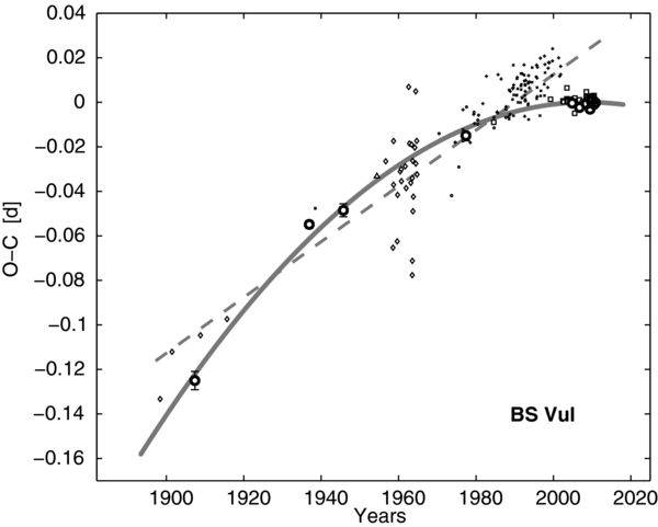
Figure 1. (O − C) diagram with respect to the linear ephemeris  , where E is an integer (epoch). Large circles with error bars correspond to "virtual times of eclipses." The small symbols "+" show published minima timings of visual observations of G. Samolyk, "×" denote timings of H. Peter, and small circles correspond to minima obtained by other visual observers (see Table 4). Small diamonds are timings of photographic plates on which the star is close to minimum and small squares are photoelectric or CCD minima timings. The dashed line corresponds to the linear ephemeris of de Bernardi & Scaltriti (1979)
  , used by visual observers.
Download figure:
Standard image High-resolution imageThe approach we applied did not use the timings of minimum light. Nevertheless, for better visualization and presentation of our results we could derive the so-called virtual times of minima and the corresponding virtual O − C values (similar to commonly used seasonal or normal values). Using the residuals of the observed data Δyi = mi − F(ti) and phase derivatives of the model function in the moment of individual observations, we can create individual values of the phase shifts. They are expressed in days (O − C)j with adapted individual weighting Wj for each observed date. An average of the phase shifts defined for arbitrarily selected groups of measurements  is then
 derived for each of eight observational sets.
  is defined as the mean shift of an observed phase curve (expressed in days) versus its model template. We assume that such introduced
  are more reliable than standard (O − C) values based on times of eclipse minima only.
3.2. Minima Timings and Their Suitability for Fine Period Analyses
The majority of eclipsing binary (EB) period studies done in the past were based on the analysis of timings of mid-eclipses. Though advanced versions of our direct period analysis method also allow for the exploitation of the radial velocity measurements and EB eclipse timings, we decided not to use these data because they did not offer anything new in the BS Vul ephemeris determination. On the contrary, using the robustly determined ephemeris given by Equation (9) we can straightforwardly discuss the properties of particular types of EB minima timings and their usability for fine period analyses.
All the BS Vul minima timings known to us are collected in Table 4, where "plate" represents the observations from photographic plates, "vis" refers to visual observations, "pe" indicates photoelectric data, and "cc" denotes CCD observations. We divided the timings, derived by several methods, into three groups: (1) timings derived from photographic plates where BS Vul seemed apparently fainter than usually (30 timings); (2) timings of minima, derived as a rule by the Kwee-van Woerden method (1956), and applied to data series acquired by objective photometric measurements (photoelectric photometry, CCD photometry, or acquiring of photographic snaps series) in a time vicinity of the predicted minima (46 timings); and (3) timings of minima derived from series of several visual estimates of the brightness of the star in the vicinity of the predicted primary minima (104 timings).
Table 4. Published Minima Timings of BS Vul
| HJDmin | Type | Filter | Number of Points | Observer | Source |
|---|---|---|---|---|---|
| (s) | |||||
| 14433.400 | plate | N. Grigorieva | PZ 5,179 (1938) | ||
| 15556.710 | pg | L. Jacchia | HB 912,22 (1940) | ||
| 18230.240 | plate | N. Grigorieva | PZ 5,179 (1938) | ||
| 20744.320 | plate | N. Grigorieva | PZ 5,179 (1938) | ||
| 28399.386 | vis | S. Piotrowski | AAC 3,68 (1937) | ||
| 29072.414 | vis | S. Piotrowski | AA 26, 341 (1976) | ||
| 31706.431 | vis | S. Piotrowski | AA 26, 341 (1976) | ||
| 34886.876 | pg | Koch & Koch | AJ 67,462 (1962) | ||
| 35718.402 | plate | H. Huth | MVS 3,114 (1965) | ||
| 36399.476 | plate | H. Huth | MVS 3,114 (1965) | ||
| 36451.385 | plate | H. Huth | MVS 3,114 (1965) | ||
| 36461.400 | plate | H. Huth | MVS 3,114 (1965) | ||
| 36807.385 | plate | H. Huth | MVS 3,114 (1965) | ||
| 36837.392 | plate | H. Busch | Hartha Beob. Zirk. 15 (1963) | ||
| 37082.527 | plate | H. Huth | MVS 3,114 (1965) | ||
| 37193.429 | plate | H. Busch | Hartha Beob. Zirk. 15 (1963) | ||
| 37202.467 | plate | H. Busch | Hartha Beob. Zirk. 15 (1963) | ||
| 37560.403 | plate | H. Huth | MVS 3,114 (1965) | ||
| 37642.260 | plate | H. Huth | MVS 3,114 (1965) | ||
| 37886.478 | plate | H. Huth | MVS 3,114 (1965) | ||
| 37959.276 | plate | H. Busch | Hartha Beob. Zirk. 15 (1963) | ||
| 38089.674 | plate | H. Huth | MVS 3,114 (1965) | ||
| 38172.510 | plate | H. Huth | MVS 3,114 (1965) | ||
| 38225.522 | plate | H. Huth | MVS 3,114 (1965) | ||
| 38231.478 | plate | H. Huth | MVS 3,114 (1965) | ||
| 38233.419 | plate | H. Busch | Hartha Beob. Zirk. 15 (1963) | ||
| 38262.461 | plate | H. Busch | Hartha Beob. Zirk. 15 (1963) | ||
| 38283.381 | plate | H. Huth | MVS 3,114 (1965) | ||
| 38323.369 | plate | H. Busch | Hartha Beob. Zirk. 15 (1963) | ||
| 38466.658 | plate | H. Huth | MVS 3,114 (1965) | ||
| 38549.502 | plate | H. Huth | MVS 3,114 (1965) | ||
| 38558.513 | plate | H. Huth | MVS 3,114 (1965) | ||
| 38640.390 | plate | H. Huth | MVS 3,114 (1965) | ||
| 38670.361 | plate | H. Huth | MVS 3,114 (1965) | ||
| 40759.411 | vis | 7 | R. Diethelm | Orion 120 (1970) | |
| 41929.317: | vis | 5 | R. Diethelm | BBSAG Bull. 11 (1973) | |
| 42275.371 | vis | 8 | R. Diethelm | BBSAG Bull. 17 (1974) | |
| 42621.390 | vis | 8 | R. Diethelm | BBSAG Bull. 23 (1975) | |
| 43011.697 | vis | 6 | K. Krueger | Obs. Min. Timings AAVSO 2 (1995) | |
| 43011.702 | vis | 8 | G. Wedemayer | Obs. Min. Timings AAVSO 2 (1995) | |
| 43011.711 | vis | 9 | G. Samolyk | Obs. Min. Timings AAVSO 2 (1995) | |
| 43271.579 | pe | V | Bernardi & Scaltriti | AAPS 35,63 (1979) | |
| 43346.795 | vis | 8 | D. Ruokonen | Obs. Min. Timings AAVSO 2 (1995) | |
| 43406.277 | pe | V | Bernardi & Scaltriti | AAPS 35,63 (1979) | |
| 43693.761 | vis | 11 | G. Samolyk | Obs. Min. Timings AAVSO 2 (1995) | |
| 44019.813 | vis | 14 | G. Samolyk | Obs. Min. Timings AAVSO 2 (1995) | |
| 44051.704 | vis | 10 | M. Baldwin | Obs. Min. Timings AAVSO 2 (1995) | |
| 44081.685 | vis | 13 | G. Samolyk | Obs. Min. Timings AAVSO 2 (1995) | |
| 44406.774 | vis | 9 | G. Hanson | Obs. Min. Timings AAVSO 2 (1995) | |
| 44407.724 | vis | 13 | G. Hanson | Obs. Min. Timings AAVSO 2 (1995) | |
| 44487.691 | vis | 17 | G. Hanson | Obs. Min. Timings AAVSO 2 (1995) | |
| 44885.607 | vis | 13 | G. Samolyk | Obs. Min. Timings AAVSO 2 (1995) | |
| 45221.654 | vis | 14 | G. Samolyk | Obs. Min. Timings AAVSO 2 (1995) | |
| 45911.7896 | pe | BV | D. R. Faulkner | PASP 98,690 (1986) | |
| 45923.691 | vis | 11 | G. Samolyk | Obs. Min. Timings AAVSO 2 (1995) | |
| 45944.629 | vis | 8 | D. Williams | Obs. Min. Timings AAVSO 2 (1995) | |
| 46230.694 | vis | 13 | G. Samolyk | Obs. Min. Timings AAVSO 2 (1995) | |
| 46270.675 | vis | 13 | G. Samolyk | Obs. Min. Timings AAVSO 2 (1995) | |
| 46321.621 | vis | 12 | G. Samolyk | Obs. Min. Timings AAVSO 2 (1995) | |
| 46606.725 | vis | 11 | G. Samolyk | Obs. Min. Timings AAVSO 2 (1995) | |
| 47059.355 | vis | 10 | A. Paschke | BBSAG Bull. 86 (1988) | |
| 47069.354 | vis | 9 | A. Paschke | BBSAG Bull. 86 (1988) | |
| 47073.639 | vis | 11 | G. Samolyk | Obs. Min. Timings AAVSO 2 (1995) | |
| 47299.720 | vis | 13 | G. Samolyk | Obs. Min. Timings AAVSO 2 (1995) | |
| 47363.499 | vis | 7 | H. Peter | BBSAG Bull. 89 (1988) | |
| 47365.416 | vis | 6 | H. Peter | BBSAG Bull. 89 (1988) | |
| 47426.329 | vis | 8 | H. Peter | BBSAG Bull. 89 (1988) | |
| 47465.369 | vis | 14 | G. Samolyk | Obs. Min. Timings AAVSO 2 (1995) | |
| 47477.258 | vis | 8 | H. Peter | BBSAG Bull. 90 (1989) | |
| 47692.403 | vis | 7 | H. Peter | BBSAG Bull. 92 (1989) | |
| 47706.687 | vis | 12 | G. Samolyk | Obs. Min. Timings AAVSO 2 (1995) | |
| 47744.765 | vis | 13 | G. Samolyk | Obs. Min. Timings AAVSO 2 (1995) | |
| 47762.386 | vis | 7 | H. Peter | BBSAG Bull. 92 (1989) | |
| 47782.354 | vis | 10 | H. Peter | BBSAG Bull. 92 (1989) | |
| 47794.743 | vis | 11 | G. Samolyk | Obs. Min. Timings AAVSO 2 (1995) | |
| 47803.306 | vis | 7 | H. Peter | BBSAG Bull. 93 (1990) | |
| 48068.421 | vis | 7 | H. Peter | BBSAG Bull. 95 (1990) | |
| 48086.508 | vis | 8 | H. Peter | BBSAG Bull. 96 (1990) | |
| 48108.410 | vis | 7 | H. Peter | BBSAG Bull. 96 (1990) | |
| 48133.637 | vis | 12 | G. Samolyk | Obs. Min. Timings AAVSO 2 (1995) | |
| 48178.373 | vis | 7 | H. Peter | BBSAG Bull. 96 (1990) | |
| 48208.353 | vis | 8 | H. Peter | BBSAG Bull. 97 (1991) | |
| 48444.434 | vis | 6 | H. Peter | BBSAG Bull. 98 (1991) | |
| 48475.385 | vis | 7 | H. Peter | BBSAG Bull. 98 (1991) | |
| 48483.471 | vis | 7 | H. Peter | BBSAG Bull. 98 (1991) | |
| 48504.412 | vis | 7 | H. Peter | BBSAG Bull. 99 (1992) | |
| 48524.405 | vis | 8 | H. Peter | BBSAG Bull. 99 (1992) | |
| 48586.275 | vis | 7 | H. Peter | BBSAG Bull. 99 (1992) | |
| 48601.517 | vis | 12 | G. Samolyk | Obs. Min. Timings AAVSO 2 (1995) | |
| 48773.822 | vis | 12 | G. Samolyk | Obs. Min. Timings AAVSO 2 (1995) | |
| 48780.481 | vis | 9 | H. Peter | BBSAG Bull. 101 (1992) | |
| 48801.421 | vis | 8 | H. Peter | BBSAG Bull. 101 (1992) | |
| 48835.675 | vis | 14 | G. Samolyk | Obs. Min. Timings AAVSO 2 (1995) | |
| 48840.444 | vis | 7 | H. Peter | BBSAG Bull. 102 (1992) | |
| 48866.620 | vis | 11 | G. Samolyk | Obs. Min. Timings AAVSO 2 (1995) | |
| 48871.387 | vis | 7 | H. Peter | BBSAG Bull. 102 (1992) | |
| 48881.382 | vis | 6 | H. Peter | BBSAG Bull. 102 (1992) | |
| 48885.663 | vis | 13 | G. Samolyk | Obs. Min. Timings AAVSO 2 (1995) | |
| 48892.323 | vis | 6 | H. Peter | BBSAG Bull. 102 (1992) | |
| 48897.558 | vis | 12 | G. Samolyk | Obs. Min. Timings AAVSO 2 (1995) | |
| 48917.558 | vis | 11 | G. Samolyk | Obs. Min. Timings AAVSO 2 (1995) | |
| 49137.445 | vis | 10 | H. Peter | BBSAG Bull. 104 (1993) | |
| 49147.450 | vis | 6 | H. Peter | BBSAG Bull. 104 (1993) | |
| 49157.446 | vis | 6 | H. Peter | BBSAG Bull. 104 (1993) | |
| 49177.427 | vis | 7 | H. Peter | BBSAG Bull. 104 (1993) | |
| 49203.618 | vis | 11 | G. Samolyk | Obs. Min. Timings AAVSO 2 (1995) | |
| 49207.406 | vis | 7 | H. Peter | BBSAG Bull. 105 (1994) | |
| 49273.580 | vis | 13 | G. Samolyk | Obs. Min. Timings AAVSO 2 (1995) | |
| 49282.626 | vis | 14 | G. Samolyk | Obs. Min. Timings AAVSO 2 (1995) | |
| 49534.414 | vis | 8 | H. Peter | BBSAG Bull. 107 (1994) | |
| 49544.416 | vis | 10 | H. Peter | BBSAG Bull. 107 (1994) | |
| 49920.428 | vis | 7 | H. Peter | BBSAG Bull. 110 (1995) | |
| 49955.655 | vis | 13 | G. Samolyk | Obs. Min. Timings AAVSO 6 (2000) | |
| 49970.395 | vis | 10 | H. Peter | BBSAG Bull. 110 (1995) | |
| 50002.290 | vis | 7 | H. Peter | BBSAG Bull. 110 (1995) | |
| 50006.578 | vis | 18 | G. Samolyk | Obs. Min. Timings AAVSO 6 (2000) | |
| 50016.565 | vis | 14 | G. Samolyk | Obs. Min. Timings AAVSO 6 (2000) | |
| 50036.569 | vis | 15 | G. Samolyk | Obs. Min. Timings AAVSO 6 (2000) | |
| 50276.436 | vis | 6 | H. Peter | BBSAG Bull. 112 (1996) | |
| 50320.727 | vis | 15 | G. Samolyk | Obs. Min. Timings AAVSO 6 (2000) | |
| 50337.369 | vis | 7 | H. Peter | BBSAG Bull. 113 (1996) | |
| 50357.362 | vis | 7 | H. Peter | BBSAG Bull. 113 (1996) | |
| 50672.457 | vis | 6 | H. Peter | BBSAG Bull. 115 (1997) | |
| 50698.648 | vis | 15 | G. Samolyk | Obs. Min. Timings AAVSO 6 (2000) | |
| 50702.438 | vis | 8 | H. Peter | BBSAG Bull. 116 (1998) | |
| 50749.573 | vis | 16 | G. Samolyk | Obs. Min. Timings AAVSO 6 (2000) | |
| 50754.329 | vis | 10 | H. Peter | BBSAG Bull. 116 (1998) | |
| 51012.774 | vis | 15 | G. Samolyk | Obs. Min. Timings AAVSO 6 (2000) | |
| 51054.668 | vis | 13 | G. Samolyk | Obs. Min. Timings AAVSO 6 (2000) | |
| 51095.604 | vis | 17 | G. Samolyk | Obs. Min. Timings AAVSO 6 (2000) | |
| 51156.528 | vis | 13 | G. Samolyk | Obs. Min. Timings AAVSO 6 (2000) | |
| 51275.9800 | ccd | A. Paschke | ROTSE, OCgate (2011) | ||
| 51411.642 | vis | 14 | G. Samolyk | Obs. Min. Timings AAVSO 6 (2000) | |
| 51452.582 | vis | 16 | G. Samolyk | Obs. Min. Timings AAVSO 6 (2000) | |
| 51460.679 | vis | 17 | G. Samolyk | Obs. Min. Timings AAVSO 6 (2000) | |
| 52042.786 | vis | 12 | G. Samolyk | Obs. Min. Timings AAVSO 10 (2004) | |
| 52133.688 | vis | 15 | G. Samolyk | Obs. Min. Timings AAVSO 10 (2004) | |
| 52225.551 | vis | 16 | G. Samolyk | Obs. Min. Timings AAVSO 10 (2004) | |
| 52235.550 | vis | 16 | G. Samolyk | Obs. Min. Timings AAVSO 10 (2004) | |
| 52448.7690 | ccd | 49 | G. Samolyk | Obs. Min. Timings AAVSO 10 (2004) | |
| 52521.5919 | ccd | 34 | G. Samolyk | Obs. Min. Timings AAVSO 10 (2004) | |
| 52803.3674 | pe | UBV | Z. Müyesseroglu et al. | IBVS 5463 (2003) | |
| 52817.4134 | pe | UBV | Z. Müyesseroglu et al. | IBVS 5463 (2003) | |
| 52831.4485 | pe | UBV | Z. Müyesseroglu et al. | IBVS 5463 (2003) | |
| 52876.6663 | ccd | 61 | R. Poklar | Obs. Min. Timings AAVSO 10 (2004) | |
| 52886.6613 | ccd | 34 | G. Samolyk | Obs. Min. Timings AAVSO 10 (2004) | |
| 52903.3198 | ccd | 45 | R. Ehrenberger | OEJV 74 (2007) | |
| 53228.4083 | ccd | C | 12 | Koss et al. | OEJV 0074 (2007) |
| 53233.6424 | ccd | 63 | J. Bialozynski | Obs. Min. Timings AAVSO 10 (2004) | |
| 53289.3324 | ccd | C | 40 | R. Ehrenberger | OEJV 74 (2007) |
| 53344.5428 | ccd | 46 | G. Samolyk | Obs. Min. Timings AAVSO 10 (2004) | |
| 53539.6916 | ccd | 48 | H. Gerner | Obs. Min. Timings AAVSO 10 (2004) | |
| 53544.4503 | ccd | I | F. Agerer | IBVS 5731 (BAVM 178) (2006) | |
| 53559.677 | ccd | 21 | S. Cook | Obs. Min. Timings AAVSO 10 (2004) | |
| 53575.3897 | ccd | C | 48 | R. Ehrenberger | OEJV 74 (2007) |
| 53579.4366 | ccd | I | F. Agerer | IBVS 5731 (BAVM 178) (2006) | |
| 53585.3848 | ccd | C | 64 | R. Ehrenberger | OEJV 74 (2007) |
| 53610.6106 | ccd | 42 | N. Simmons | Obs. Min. Timings AAVSO 10 (2004) | |
| 53615.3710 | ccd | I | F. Walter | IBVS 5731 (BAVM 178) (2006) | |
| 53616.3221 | ccd | C | 69 | R. Ehrenberger | OEJV 74 (2007) |
| 53946.6452 | ccd | 65 | G. Samolyk | Obs. Min. Timings AAVSO 12 (2007) | |
| 54003.2869 | ccd | R | 70 | R. Ehrenberger | OEJV 74 (2007) |
| 54302.6708 | ccd | 65 | G. Samolyk | Obs. Min. Timings AAVSO 12 (2007) | |
| 54318.3781 | ccd | I | 76 | F. Walter | IBVS 5830 (BAVM 193) (2008) |
| 54596.8208 | ccd | C | 87 | G. Samolyk | JAAVSO 36,186 (2008) |
| 54637.7543 | ccd | C | 60 | J. Bialozynski | JAAVSO 36,186 (2008) |
| 54649.4172 | ccd | R | 166 | R. Ehrenberger | OEJV 94 (2008) |
| 54658.4630 | ccd | I | 41 | F. Agerer | IBVS 5889 (BAVM 203) (2009) |
| 54684.3989 | ccd | I | 84 | F. Walter | IBVS 5889 (BAVM 203) (2009) |
| 54688.6830 | ccd | C | 68 | G. Samolyk | JAAVSO 36,186 (2008) |
| 54709.6259 | ccd | C | 68 | G. Samolyk | JAAVSO 36,186 (2008) |
| 54712.4825 | ccd | I | 65 | F. Agerer | IBVS 5889 (BAVM 203) (2009) |
| 54770.5500 | ccd | 86 | G. Samolyk | JAAVSO 37,44 (2009) | |
| 55005.6791 | ccd | 93 | G. Samolyk | JAAVSO 38, 85 (2010) | |
| 55071.3633 | ccd | C | 30 | H. Jungbluth | IBVS 5941 (2010) |
| 55146.5658 | ccd | G. Samolyk | JAAVSO 38, 183 (2010) | ||
| 55380.7456 | ccd | G. Samolyk | JAAVSO 39,94 (2011) | ||
| 55405.2547 | ccd | Rc | 286 | K. Shiokawa | VS Bull. VSOLJ No. 51 (2011) |
| 55483.3142 | ccd | I | 57 | L. Šmelcer | OEJV 137 (2011) |
| 55483.3152 | ccd | Rc | 57 | L. Šmelcer | OEJV 137 (2011) |
The scatter of times in the first group (1) is rather large: σ(O − C) = 0.020 days, nevertheless the mean value of (O − C) is close to zero:  days. The second group of observations (2) display an excellent agreement with our quadratic ephemeris (see Equation (9)). We found that
  days, the standard deviation of the scatter σ(O − C) = 0.0019 days. The standard deviation of visually determined minima timings (3) is of a moderate value: σ(O − C) = 0.0085 days. The corresponding weights of these three types of determination of minimum light should be in the ratio 1:110:5.6!
However, too credulously handling visually determined EB minima timings proved to be sometimes a rather hazardous business. Such data suffer from a lot of bad attributes that effectively limit their suitability for fine period analysis purposes. We can enumerate only the most serious ones.
- 1.Because of the poor quality of visual observations themselves the corresponding accuracy of the eclipse time determination used to be much worse than in the case of other types of photometric observations. The quality of visual timings used to be further deteriorated by the fact that some determinations were based on only a few individual observations done only in the immediate vicinity of the predicted time of minima. This is typical for some observers and one should be careful when using such unreliable minima timings. See the numbers of estimates used for minima timings determinations in Table 4.
- 2.The timings of minima of the time series of visual estimates often used to be determined by obscure, irreproducible methods. In the worst case, the original estimates were not published and they are now inaccessible.
- 3.Almost all methods developed for the processing of astrophysical observations are based on an application of LSM. Unfortunately, the method strictly requires that subsequent estimates are independent. This requirement is not met in time series of visual observations. "Observed" visual light curves are subjectively smoothed to the ideal of theoretical or photoelectric light curves with clearly defined descending and ascending branches. This smoothing therefore prevents us from estimating the real uncertainty of the timings' determination from the time series of only one observing session. The uncertainties formally calculated and published from the smoothed light curve data are many times smaller than they should be.
- 4.The most severe flaw in the majority of the visual observations is that observers obviously knew the predicted time of minimum light to an accuracy of minutes. If the ephemeris for the time of minimum light was incorrect, most observers were influenced into confirming the predicted, incorrect time of minimum light. This subjective effect, which is able to completely depreciate observations, equally afflicts both beginners and "experienced" visual observers.
The above general starting points are based on our long-standing experience with visual observations of EBs. Two of us (Z.M. and M.Z.) are now preparing an essential study on the reliability of visual EB timings and their usability for period analysis, where all the above-mentioned points of discussion will be studied and documented in detail for many assorted cases.
Analyzing 104 visual timings listed in Table 4 from 1970 to 2003 we found that they correlated very well with the linear ephemeris of de Bernardi & Scaltriti (1979)  , that was generally used by visual observers for their observation schedule (see Figure 2). The linear fit of visual observations is almost parallel with the line of prediction, while timings of minima systematically lag behind the minimum forecast by several minutes. Visual observations have only a very weak correlation with the real quadratic ephemeris. The conclusion is obviously valid for almost all visual observers who targeted the star. It is apparent that practically all visual observers subjectively adjusted their observations to more or less confirm the existing ephemeris.
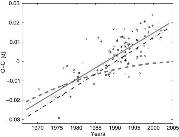
Figure 2. (O − C) diagram of visually determined primary eclipse timings with respect to the linear ephemeris  , where E is an integer (epoch). The "+" symbols show G. Samolyk timings, "×"s denote H. Peter timings, and circles correspond to timings obtained by other visual observers. The dash-dotted line corresponds to the linear ephemeris of de Bernardi & Scaltriti (1979) JDI = 2443271.578 + 0.47597147 × E, used by visual observers. The dashed curve is the real quadratic course. The full line is the linear fit of visually determined timings; dotted lines are the 1σ uncertainty of this fit.
Download figure:
Standard image High-resolution imageThe apparent "delay" in visual observers' timings with respect to the prediction agrees well with the heliocentric corrections for the times of observation. Observers used geocentric time, but the predicted minimum light time was heliocentric time, which was delayed via geocentric time by several minutes on the night when observations were done.
The most active visual observer of BS Vul, G. Samolyk, also published on the AAVSO Web site 528 brightness estimates obtained during his observations of 39 primary eclipses of BS Vul in the time interval of 1984–2002. We analyzed all these data in detail and arrived, i.e., at the following conclusions.
- 1.Observations of BS Vul were always optimally scheduled, typically 12 estimates per eclipse were able to describe the complete eclipse quite well. Both descending and ascending branches of the light curve during eclipses were covered nicely.
- 2.The resulting light curves were perfectly symmetric and they corresponded very well with ideal photometrically acquired curves. Samolyk light curves were very smooth; their scatter derived from the form of the light curve is only 0.055 mag! However, the scatter of individual times of eclipses indicates that the real scatter in estimates should be at least five times larger!
- 3.The scatter of timings published by Samolyk and their bad affinity to the real quadratic ephemeris might have been caused by the application of an inappropriate method for the derivation of light curve minima from estimate series. We apply our own rigorous method to determine the times of minima when we know the light curve shape (Mikulášek et al. 2011b). We obtained diverse times of minima. Nevertheless, all of them were clustered around the de Bernardi & Scaltriti (1979) ephemeris. Consequently, the estimates themselves were biased to accommodate the forecast.
- 4.It is evident that our findings prove the heavily subjective character of visual observations of short-period EBs, which disqualifies them as a source of unbiased information apt for fine EB period analyses.
On the other hand, we could use 200 visual estimates of brightness made by S. Piotrowski in two time intervals (1935–1939 (155 estimates) and 1945–1946 (45 estimates)), because these estimates have a different character than later AAVSO and BBSAG visual observations. The distribution of these old visual estimates shows that they were obtained in "monitoring mode" without the primary aim to obtain minima timings. Furthermore, they passed our careful analysis.
4. PHOTOMETRIC SOLUTION OF BS Vul
The new complete  CCD light curves of BS Vul were analyzed by the 2003 version of the Wilson–Van Hamme code (Wilson & Van Hamme 2003). During the computation, each band of CCD observations was binned into 100 normal points for every 0.01 phase interval, and the number of observations in each bin was adopted as the weight of the normal point. The corresponding light curves are shown in Figure 3. Given the F2 spectral type of BS Vul, we assumed an effective temperature of T1 = 7 000 K for the primary component (the star eclipsed at primary minimum). We took the gravity-darkening coefficients as g1 = g2 = 0.32 (Lucy 1967) and the bolometric albedo as A1 = A2 = 0.5, corresponding to the convective envelope of this binary system. Bolometric and bandpass square-root limb-darkening parameters were taken from Van Hamme's paper (1993). The adjustable parameters are the inclination
  , the mean temperature of star 2, T2; the monochromatic luminosity of star 1, L1B, L1V, L1I, and L1R; and the dimensionless potentials of stars 1 and 2, Ω1 and Ω2.

Figure 3. Observed and theoretical BV(IR)c light curves of BS Vul. The panel on the right shows a close-up comparison of the data to model light curves with, and without, a hot spot on the secondary component.
Download figure:
Standard image High-resolution imageSince no accurate mass ratio for BS Vul had been published, we needed to search for a reliable mass ratio, q, via the differential correction program. From Figure 3, one can see that the duration of the bottom of the primary eclipse is about 50 minutes, indicating that the eclipse is total. This characteristic makes the photometric mass ratio reliable. For searching the mass ratio q, the solutions for several assumed values of the mass ratio were obtained. For each q, the calculation starts at mode 2 (the detached mode). The sums of weighted square deviations Σ Wi (O − C)2i for all the assumed values of q are shown in Figure 4. The minimum Σ is achieved at q = 0.34 for BS Vul with mode 4 (the semidetached case with the primary component filling the critical RL). Therefore, we performed a differential correction so that the calculation converges by making q an adjustable parameter and by choosing q = 0.34 as the initial value. Finally, the converged photometric solutions were obtained as listed in the second column of Table 5. The values are given together with their uncertainties shown in parentheses. The theoretical light curves computed with these values are plotted in Figure 3 with solid lines.

Figure 4. Σ − q curves of BS Vul.
Download figure:
Standard image High-resolution imageTable 5. Photometric Solutions of BS Vul
| Parameters | Unspotted | Spotted |
|---|---|---|
| g1 = g2 | 0.32 | 0.32 |
| A1 = A2 | 0.5 | 0.5 |
| i (deg) | 88.4(9) | 87.8(8) |
| T1 (K) | 7000 | 7000 |
| T2 (K) | 4644(18) | 4632(18) |
| q | 0.340(3) | 0.340(4) |
| Ω1 | 2.5530 | 2.5530 |
| Ω2 | 2.5549(13) | 2.5651(46) |
| L1B/(L1B + L2B) | 0.9761(3) | 0.9771(3) |
| L1V/(L1V + L2V) | 0.9560(3) | 0.9576(3) |
| L1I/(L1I + L2I) | 0.9202(3) | 0.9226(3) |
| L1R/(L1R + L2R) | 0.9452(3) | 0.9400(3) |
| φ (deg) | 90(fixed) | |
| θ (deg) | 96.1(6.9) | |
| rs (deg) | 37(11) | |
| Ts/T* | 1.18(12) | |
| Σ | 0.0246 | 0.0218 |
Download table as: ASCIITypeset image
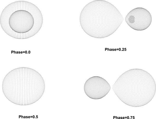
It is evident from Figure 3 that the theoretical light curves do not fit the observations very well over the phase 0.25–0.45 for BS Vul. This phenomenon could be the result of the mass transfer from the primary component to the secondary via a stream heating the facing hemisphere of the secondary component. With the addition of a hot spot on the secondary star near the inner Lagrange point, we found that our solutions converged. The corresponding solutions are listed in Column 3 of Table 5. The spot parameters are latitude, φ, longitude, θ, angular radius, rs, and the temperature factor, Ts/T* (where Ts is the temperature of the spot and T* is the local effective temperature of the adjacent photosphere). Corresponding synthetic light curves are depicted in Figure 3 with dashed lines and shown more clearly in the right-hand panel of this figure. From Figure 3, one can see that the additions of spots give better fits to the observed light curves. Our photometric solutions indicate that BS Vul is a near contact binary system with the primary component filling its critical RL and the secondary component close to filling its RL, but still detached. The configurations of BS Vul with a hot spot are pictured in Figure 5.
Figure 5. Configuration of BS Vul at phases of 0.00, 0.25, 0.50, and 0.75.
Download figure:
Standard image High-resolution image
5. DISCUSSION AND CONCLUSION
Based on our good quality BV(IR)c light curves, the photometric solutions for BS Vul are derived. It is shown that BS Vul is a primary filling near contact binary system (i.e., SD1 NCB). The excess luminosity seen in the light curves on the ingress of the secondary minimum can be explained by a hot spot on its secondary component near the inner Lagrangian point, which could be attributed to the mass flow from the primary component to the secondary one via a stream heating the facing hemisphere of the secondary component, just like other SD1 NCBs (see Zhu et al. 2009). Since no spectroscopic elements have been published for BS Vul, its absolute parameters cannot be determined directly. Assuming that the primary component is a normal, main-sequence star, we can estimate its mass as 1.52 M☉, corresponding to its spectral type of F2 (Cox 2000). Combined with the photometric solutions and its period, we then estimated the absolute parameters for this system as M2 = 0.52 M☉, R1 = 1.54 R☉, R2 = 0.93 R☉, L1 = 5.13 L☉, and L2 = 0.35 L☉.
We did the period analysis using our own method. In our approach, we used all available individual measurements instead of minima timings only because that allows us to obtain more information from the data and to study the quality of the data simultaneously. We found that the orbital period of this system is decreasing at a rate of dP/dt = (− 0.00211 ± 0.00006) s yr−1, which implies a continual mass flow from the primary component to the secondary one at a rate of dM/dt = (1.69 ± 0.04) × 10−8 M☉ yr−1 assuming the conservative case. The period decrease found in this system is consistent with its primary filling semidetached configuration and the asymmetrical shapes of its light curves. With the absolute parameters, the thermal timescale of the primary component can be estimated to be GM2/RL ∼ 1 × 10⁷ years, which is approximate to the timescale of period decrease P/(dP/dt) ∼ 1.6 × 10⁷ years. It implies that the mass may transfer on the thermal timescale.
With the orbital period decrease, the primary component transfers mass to the secondary one, the mass ratio increases and eventually the present semidetached system BS Vul may evolve into the contact phase. Therefore, it is possible that BS Vul is a progenitor of an evolved contact binary, or is in a broken-contact stage, just like BL And (Zhu & Qian 2006), CN And (Lee & Lee 2006), and V473 Cas (Zhu et al. 2009), etc., which is predicted by the theory of thermal relaxation oscillations (TRO; Flannery 1976; Lucy 1976 and Lucy & Wilson 1979). According to TRO theory, W UMa systems must undergo oscillations around the state of marginal contact. Each oscillation comprises a contact phase followed by a semidetached phase. When a system exhibits β Lyrae-type light-variation departures from EW light curves, a semidetached phase, with the more massive star filling the RL, followed by a marginal-contact phase with poor thermal contact, is to be expected. Thus, BS Vul is another good observational example supporting the TRO theory.
Our analysis of mid-eclipse timings of BS Vul derived from the time series of visual observations proved the heavily subjective character of visual observations of BS Vul. We conclude that visual observations (minima timings) of short-periodic EBs cannot be used as a source of unbiased information appropriate for fine EB period analysis without very careful preliminary verification.
This study was partly supported by the Chinese Natural Science Foundation (Nos. 11133007, 10973037, and 10903026) and by the grants MŠMT LH12175, GAČR P209/12/0217, and MUNI/A/0968/2009.