The electric field distribution in the brain during TTFields therapy and its dependence on tissue dielectric properties and anatomy: a computational study

Cornelia Wenger; Ricardo Salvador; Peter J Basser; Pedro C Miranda

doi:10.1088/0031-9155/60/18/7339

1. Introduction

Tumour Treating Fields (TTFields) are alternating electric fields of intermediate frequencies (100–300 kHz) with intensities between 1 and 3 V cm⁻¹ that are delivered via capacitively coupled transducer arrays. This non-invasive and anti-mitotic treatment is intended to selectively target dividing cells. TTFields were approved in 2011 by the U.S. Food and Drug Administration (FDA) for the treatment of recurrent glioblastoma multiforme (GBM).

The application of TTFields leads to distinct biophysical effects observed during in vitro experiments. Kirson et al (Kirson et al 2004) reported that when cells were treated with TTFields, not only was the mitotic phase prolonged or completely arrested, but a variety of abnormal mitotic figures were also observed. Additionally if the cell proceeded to telophase, then membrane blebbing and rupture occurred in one fourth of the tested cells, leading to cell death.

TTFields are thought to disrupt the proper assembly of the mitotic spindle by interfering with polymerization of microtubules. Their tubulin dimers are one of the most polar intracellular components and therefore most susceptible to applied electric fields. Furthermore, during cytokinesis the hourglass cell shape produced as the daughter cells are formed induces a non-uniform electric field with increased field strength at the furrow region. This field results in dielectrophoretic forces that may move polar and charged molecules within the cytosol, thus compromising normal cytokinesis (Gutin and Wong 2012, Wenger et al 2014b).

In vitro experiments performed with various cancer cell lines showed that the effect of TTFields is dependent on the frequency, the field intensity, and the orientation of the applied field (Kirson et al 2004, 2007). For each cell line there appears to be an optimal frequency for which the inhibitory effect on cell division is greatest, e.g. for glioma cells a frequency of 200 kHz leads to the greatest reduction in cell proliferation (Kirson et al 2007). Furthermore, the inhibitory effect of TTFields starts at 1 V cm⁻¹ and increases with increasing field intensity. Complete proliferation arrest for rat glioma cells was seen after a 24 h exposure to TTFields of 2.25 V cm⁻¹ (Kirson et al 2004). Concerning the orientation dependence, TTFields are most effective when the applied electric field and the axis of cell division are parallel (Kirson et al 2004). Since these axes are randomly orientated in the tumour, multiple field directions are alternately applied to improve efficacy: two perpendicular field directions were found to be about 20% more effective than a single direction (Kirson et al 2007). The anti-tumour effect of TTFields was also demonstrated in animal tumour models (Kirson et al 2007).

The Optune^™ device was developed by Novocure (www.novocure.com) to deliver TTFields in human subjects by means of two pairs of perpendicular transducer arrays that are sequentially switched. Both array pairs are placed on the patient's shaved scalp, one operating in the left and to the right (LR) direction and one in the anterior and posterior (AP) direction (figure 1). The arrays are connected to a field generator (Fonkem and Wong 2012). It is recommended that TTFields should be applied continuously.

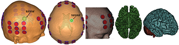
**Figure 1.** Realistic human head model of s2. The tumour position is illustrated for two different views. At the right, the meshes representing the scalp and selected transducers, the WM, and the GM with the cerebellum are shown.
Download figure:
Standard image High-resolution image

The results of the first small pilot trial, in which 10 patients with recurrent GBM received TTFields as a monotherapy were encouraging and indicated that the use of TTFields was safe (Kirson et al 2007). In the first phase III trial (EF-11) TTFields were compared to physician's choice chemotherapy in a total of 237 recurrent GBM patients. TTFields were found to be equally effective as chemotherapy with no drug toxicity, and thus associated with better quality of life status of the patients (Stupp et al 2012). This trial lead to the approval of the Optune^™ system for the treatment of recurrent GBM by the FDA. The analysis of a patient registry dataset (PRiDe) with 457 recurrent GBM patients who were treated with TTFields showed that ⩾75% compliance, i.e. application for ⩾18 h d⁻¹, was a favourable prognostic factor (Mrugala et al 2014). A recent Phase III clinical trial (EF-14) of TTFields in patients with newly diagnosed GBM was terminated during interim analysis due to early success (Stupp et al 2014). In this study patients treated with TTFields in combination with the chemotherapeutic agent temozolomide (TMZ) demonstrated a significant increase in progression-free survival and overall survival compared to TMZ alone. The EF-14 trial investigators proposed that TTFields/TMZ should become the new standard of care for GBM (Stupp et al 2014).

As already noted, the efficacy of TTFields therapy depends on the electric field strength that can be delivered to the tumour. While the field intensity can be measured in cell cultures and animals, its assessment inside the human head remains problematic. Currently only one intracranial measurement exists showing that an electric field strength of 1–2 V cm⁻¹ within the centre of the brain can be produced by applying a 50 V difference between the transducer arrays (Kirson et al 2007). However, the electric field distribution can be predicted using realistic computational models of the human head. We have already shown that the electric field distribution within the brain induced by TTFields is highly non-uniform. The induced field was calculated to be higher than 1 V cm⁻¹ in over 60% of the brain. Furthermore, different field strengths in a virtual lesion that represents a tumour were predicted for the LR and AP array pairs (Wenger et al 2013, 2014a, Miranda et al 2014). These studies were based on a single subject, and incorporated isotropic values for the conductivities and permittivities that were obtained from the literature. However, white matter anisotropy has been shown to influence the electric field distribution in the brain in related techniques such as electroconvulsive therapy (Lee et al 2011) and transcranial direct current stimulation (tDCS) (Suh et al 2012, Shahid et al 2013, 2014), and is expected to affect TTFields distribution in the brain, as well. Also, isotropic conductivity values are not known accurately since a wide range of values are reported in the literature (see Methods).

For this study we developed a second realistic human head model from an MRI dataset that included diffusion tensor imaging (DTI) data as a means to estimate the anisotropic and heterogeneous conductivity distribution. This follows the proposition that the conductivity tensors share the same eigenvectors as the effective diffusion tensor (Basser et al 1994). In addition, the DTI pipeline for calculating eigenvectors, eigenvalues, mean diffusivities (Basser et al 1994) and the fractional anisotropy (Pierpaoli and Basser 1996) is extensively used in this work.

With these models, we started investigating the effect of conductivity anisotropy on the electric field distribution in TTFields applications, particularly on the electric field strength in the virtual tumour. Additionally, we carried out a sensitivity analysis to determine how uncertainties in the dielectric properties of tissues affect the electric field in the tumour. Finally, we compared the two realistic head models to examine inter-subject differences in the field distribution for the same tumour location and size, and the same transducer array layout.

2. Methods

2.1. Development of a new head model

One realistic human head model has already been developed based on T₁ and proton density (PD) MR images of a healthy young male subject, as described in (Miranda et al 2013). A second realistic head model was developed from the MRIs of a 20 year-old healthy female subject. This dataset consisted of T₁ − (TR = 2050 ms, TE = 3.09 ms) and T₂ − (TR = 6000 ms, TE = 429 ms) weighted MR images with 1 mm³ isotropic resolution, acquired on a Siemens MAGNETOM Avanto 1.5 T scanner. Additionally, a DTI dataset (TR = 7500 ms, TE = 113 ms, b-value = 1000 s mm⁻² applied in 20 non-collinear directions) was acquired with 1.25 mm × 1.25 mm × 3.5 mm anisotropic voxel resolution. First, the images were registered to MNI (Montreal Neurological Institute) space with FSL FLIRT (Jenkinson et al 2012). The grey matter (GM) and white matter (WM) surface meshes were created using the SimNibs pipeline (Windhoff et al 2013) with minor adaptations. The software package Brainsuite (Shattuck and Leahy 2002), version 13, was used to obtain surface meshes of the cerebrospinal fluid (CSF), the skull and the scalp. Furthermore, the surface meshes were corrected for triangle intersection, unnatural bumps and holes with Mimics, (v16.0, www.materialise.com).

In Mimics, a virtual tumour within the right hemisphere, near a lateral ventricle and totally contained in the WM (figure 1), was positioned as close as possible to the virtual tumour placed in the first subject. The cystic tumour was represented by two concentric spheres, incorporating a necrotic core of 1.4 cm diameter within a 2.0 cm active shell. Additionally, the transducer arrays were modelled so as to represent the Optune^™ system as closely as possible. Each transducer was modelled as a 1 mm high ceramic disc with a diameter of 9 mm. Each array consisted of 3 × 3 transducers separated by 22 mm and 33 mm along two perpendicular directions. A thin layer of conductive gel (0.5–2 mm) of 10 mm diameter was placed underneath each transducer (figure 1). Finally, Mimics was also used to transform the assembly of all surface meshes into a volume mesh, suitable for finite element method (FEM) analysis. This model had approximately 6.1 million degrees of freedom.

We will refer to the first model as subject 1 (s1) and the second model as subject 2 (s2).

2.2. Dielectric properties and processing of DTI data

Conductivity and permittivity values at 200 kHz were obtained through an extensive literature search for all the tissues represented in the model: scalp (Hemingway and McClendon 1932, Burger and van Milaan 1943, Yamamoto and Yamamoto 1976, Gabriel et al 1996), skull (Kosterich et al 1983, Reddy and Saha 1984, De Mercato and Garcia Sanchez 1992, Law 1993), CSF (Crile et al 1922, Gabriel et al 1996, Baumann et al 1997), GM and WM (Freygang and Landau 1955, Ranck 1963, Van Harreveld et al 1963, Stoy et al 1982, Surowiec et al 1986, Latikka et al 2001, Logothetis et al 2007, Gabriel et al 2009), and tumour (Peloso et al 1984, Surowiec et al 1988, Lu et al 1992, Latikka et al 2001). The ventricles were assumed to be filled with CSF. For each tissue a range of isotropic values is reported in the literature, so standard, minimum and maximum values for each parameter were chosen to be used in this study (table 1). The standard values are the same as those used in a previous study (Miranda et al 2014), for which model s1 was first produced.

Table 1. Standard maximum and minimum values of dielectric properties of tissues, transducers and gel.

	Conductivity σ (Sm⁻¹)			Rel. permittivity ε
	Min	Standard	Max	Min	Standard	Max
Scalp	0.14	0.25	0.45	1000	5000	10 000
Skull	0.003	0.013	0.032	50	200	300
CSF	1.64	1.79	1.94	100	110	110
GM	0.15	0.25	0.50	2000	3000	3800
WM	0.08	0.12	0.30	1000	2000	3000
Shell	0.15	0.24	0.50	—	2000	—
Core	0.50	1.00	1.50	—	110	—
Gel	—	0.10	—	—	100	—
Transducer	—	0	—	—	10 000	—

For s2, the DTI data was used to estimate the anisotropic conductivity tensors for GM and WM following the SimNibs pipeline. First, the FSL diffusion toolbox (Smith et al 2004) was used for correction and registration of the images and calculating the principal directions (eigenvectors), principal diffusivities (eigenvalues), and the fractional anisotropy, as described in (Windhoff et al 2013). Subsequently the SimNibs Matlab scripts were adapted to estimate the corresponding conductivity tensors with our baseline conductivity of the WM and the GM (table 1). As described in detail in (Opitz et al 2011), two ways of estimating the conductivity tensors are used. The direct mapping (dM) method (Tuch et al 2001) assumes a linear relationship between the eigenvalues of the diffusion and conductivity tensors, i.e. σ_v = s⋅d_v, where s is a constant, and σ_v and d_v are the vth eigenvalues of the conductivity and the diffusion tensors respectively. An adapted scaling factor s is applied following (Rullmann et al 2009). In our model with the standard conductivities in table 1 this factor resulted in s = 0.224 [S⋅s mm⁻³]. The second approach follows the proposal of (Güllmar et al 2010) which will be referred to as volume normalized (vN) mapping since the geometric mean of the conductivity tensor's eigenvalues in each voxel in the brain (WM and GM, including the cerebellum) are matched locally to the specific isotropic conductivity values. These two methods result in different conductivity tensors. The xx and yy-component of the tensors, which correspond to the apparent diffusivities or conductivities along the LR (x-axis) and AP (y-axis) directions are illustrated in figure 2. The average of all mean conductivity values within the whole brain is similar for the two methods, i.e. the whole-brain average value of the trace of the conductivity tensor divided by 3 is 0.195 S m⁻¹ in the dM model and 0.182 S m⁻¹ in the vN model. Yet, regional differences between GM and WM are clearly visible in figure 2, and are also reflected in the average conductivity values that are produced by the two mapping methods for these tissues. For dM, the mean conductivity is 0.175 S m⁻¹ within the WM and 0.215 S m⁻¹ within the GM, whereas the corresponding values in the vN model are 0.127 S m⁻¹ and 0.252 S m⁻¹ and thus are similar to the isotropic values. The percentage difference between mean conductivity values in GM and WM is only 21% in the dM method, but 66% in the vN model.

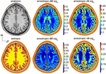
**Figure 2.** An axial slice above the tumour is shown in the anatomic image on the top left. The corresponding isotropic conductivity map is plotted below, in arbitrary colours—isotropic conductivity values are presented in table 1. For the anisotropic brain tissues, the dM tensor components are shown in the middle and vN in the right columns, respectively. Top panels illustrate the xx-component of the tensor, the bottom panels the yy-component of the tensor. The colour scale applies to GM and WM only. All conductivity values are given in Sm⁻¹.
Download figure:
Standard image High-resolution image

2.3. Solution of the model

In order to calculate the electric field distribution within the brain the FEM model was used to solve the electroquasistatic approximation of Maxwell's equations (Haus and Melcher 1989), which is valid for our experimental conditions. For this FEM model we utilized the Electric Currents Interface of Comsol Multiphysics, version 4.3b (www.comsol.com), which solves a current conservation problem for the scalar electric potential. Within this package it is now possible to formulate the time-harmonic problem as a stationary problem in the frequency domain with complex-valued solutions. The frequency was set to 200 kHz.

The following boundary conditions were imposed: continuity of the normal component of the current density at all interior boundaries and electric insulation at the external boundaries. The active transducers were modelled as current sources. Their external bases were simulated with the floating potential boundary condition that sets the potential at that boundary so that the integral of the normal component of the current density is equal to the specified amplitude of 100 mA per transducer. In practice, the Optune^™ system operates in a slightly different mode since the total current is controlled at the array level (900 mA) and not at the transducer level.

3. Results

In order to analyse differences in the electric field distribution quantitatively the average and maximum values of the electric field strength (in V cm⁻¹) were evaluated for the different tissues. Additionally, the percentage of a tissue volume where the field intensity exceeded a specified threshold was calculated. These quantities will be referred to as above-threshold-volumes, i.e. the abbreviations ATV1, ATV2 and ATV3 correspond to the percentage of tissue volume with an electric field magnitude greater than 1 V cm⁻¹, 2 V cm⁻¹ and 3 V cm⁻¹, respectively.

3.1. Isotropic versus anisotropic conductivities

The impact of anisotropic conductivity on the electric field distribution was analysed based on three versions of model s2: one with isotropic conductivity values and two with anisotropic GM and WM values (vN and dM). The results in figure 3 show that field distributions are similar for all three models. However, the field in the brain in the vN model is generally higher than in the other two models, because of the higher difference in conductivity values of GM and WM generated by this mapping method. Conversely, the field in the dM model is generally lower than in the other two models, because of the lower difference in conductivity values generated by this mapping method.

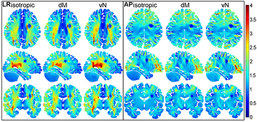
**Figure 3.** Electric field strength (V cm⁻¹) distribution in s2. Axial (top row), sagittal (middle row) and coronal (bottom row) slices through the spherical tumour for the LR (left panel) and AP (right panel) stimulations. Isotropic results are plotted on the left and corresponding anisotropic results for vN and dM are illustrated in the middle and right columns respectively. The colour range is the same for all figures and varies between 0 (dark blue) and 4 (dark red) V cm⁻¹.
Download figure:
Standard image High-resolution image

The average values of the electric field magnitude in the brain, the tumour shell and the tumour core are given in table 2 for both array configurations. As expected from figure 3, the average value of the electric field in the brain is higher for the vN model and equal or lower for the dM model, in comparison to the isotropic model. On the other hand, the average value of the electric field in the tumour shell (and also in the tumour core) is higher in both anisotropic models than in the isotropic model. This pattern is observed in both array configurations. For this particular tumour location and array setup, the average field within the tumour tissues is higher for the LR configuration in all isotropic and anisotropic models. Conversely, the average field in the brain is always higher for the AP configuration. In the tumour shell, the average electric field is increased to approximately 111% of the isotropic value for the LR configuration and to 106% for the AP configuration in the dM model, and to 106% for LR and 102% for AP in vN model respectively.

Table 2. Average field strength (V cm⁻¹) in the brain and tumour for the isotropic and anisotropic models.

		Brain	Shell	Core
LR	iso	1.41	1.59	0.74
	dM	1.39	1.76	0.82
	vN	1.45	1.68	0.78
	dM/iso	98%	110%	111%
	vN/iso	103%	106%	106%
AP	iso	1.43	1.13	0.52
	dM	1.43	1.20	0.55
	vN	1.49	1.15	0.53
	dM/iso	100%	106%	106%
	vN/iso	104%	102%	101%

The ATVs in table 3 also show that the anisotropy of WM and GM has a limited impact on the electric field distribution in the tumour shell. Anisotropy generally leads to higher predicted ATV values, particularly ATV1 for the AP arrays and ATV2 for the LR arrays. However, the main difference is due to the array configuration. The higher electric field values achieved in the LR configuration result in larger tumour volumes being exposed to a field of more than 1 V cm⁻¹.

Table 3. Comparison of ATVs in the tumour shell for the isotropic and anisotropic models.

	LR setup			AP setup
	iso	dM	vN	iso	dM	vN
ATV1	91%	92%	90%	58%	65%	58%
ATV2	17%	28%	23%	1%	2%	2%
ATV3	3%	6%	4%	0%	0%	0%

The incorporation of anisotropy in the model also influenced the maximum electric field values. The maximum values in the brain were even more affected than the average values and showed large differences for the dM, vN and isotropic conductivity values. On the other hand, the increase in the maximum field strength in the tumour tissues when incorporating anisotropy remained comparable to those of the average field strength, because the tumour tissues were always considered to be isotropic.

3.2. Sensitivity to tissue dielectric properties

As shown in table 1, the dielectric properties of tissues are not known precisely so we performed a sensitivity analysis to determine how their changes in different tissues affected the electric field distribution. This analysis was performed on the anisotropic versions of model s2. A new set of conductivity values was generated by changing the conductivity of one tissue to the maximum or the minimum value in table 1, while all the other parameters retained their standard value. In the case of GM and WM, the conductivity tensors for both methods had to be recalculated for each new combination of GM and WM isotropic values. For each new parameter set the model was evaluated for both anisotropic conductivity mapping methods and also for both active array configurations. The same analysis was carried out for changes in permittivity.

One general finding was that the average and maximum electric field values as well as the three ATVs were similar or higher in the vN model compared to the dM model for almost all tissues. The noteworthy exceptions were the tumour tissue and the GM, for which the dM model produces higher values. Nonetheless within the total volume of the brain the vN values exceed the dM values due to the contribution of the WM. As an example, figure 4 shows ATV1 plotted as a function of scalp conductivity. In the tumour shell (left) the solid curves that correspond to the vN model are lower than the dotted dM curves, whereas in the brain parenchyma (right) the opposite is true.

**Figure 4.** ATV1 in the tumour shell (left) and brain parenchyma (right) as a function of scalp conductivity. Results are presented for LR (blue) and AP (green) setups for both anisotropic models, vN (solid) and dM (dotted).
Download figure:
Standard image High-resolution image

Another observation is that the vN and dM curves have similar shapes, i.e. the effect of changing conductivity is almost the same for both mapping methods. In other words, the ratio of the maximum to minimum ATV volumes does not depend strongly on the conductivity mapping method used (but the absolute values do). This can be seen in figure 4 for the specific case of changes in the scalp conductivity. This general tendency was also observed in the plots of the average electric field. Again there exists an exception which concerns conductivity changes of the GM and WM that have varying impact for dM and vN, but only on the brain tissue itself.

The effects of variations in the conductivity of each tissue on the average electric field in the brain and in the tumour shell are presented in figure 5. The plots show the changes in average electric field in the tumour shell, (a) and (b), and in the brain, (c) and (d), that result from changes in the conductivity of one of the tissues, for both the LR, (a) and (c), and the AP array configurations, (b) and (d). Scaled conductivities are plotted along the x-axis, where the value 1 corresponds the standard value of each conductivity. Since different ranges were defined for the conductivity of the various tissues, the curves are unequal in length. The 3 numbers in the plot area are the lowest and highest detected average electric field values, and the average electric field value for the standard conductivity values. Figure 5 only displays the dM curves, but although the results are mostly similar, different outcomes obtained by dM and vN methods will be pointed out later on.

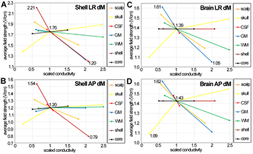
**Figure 5.** Average electric field strength for varying conductivities of all tissues, obtained with the dM method. The x-axis corresponds to the scaled conductivity values, from table 1. The results for the tumour shell are presented in the left column, the ones for the brain tissue in the right column. Results for LR and AP configurations are shown in the top and bottom rows, respectively.
Download figure:
Standard image High-resolution image

Increased scalp conductivity led to lower values of electric field strength and ATVs everywhere. This is due to more current between the two arrays being shunted through this tissue, and therefore less flowing across the skull into the cranial cavity. For the tumour shell and AP stimulation (figure 4 left, red curves) the ATV1 reduces from about 75% and 80% for low scalp conductivity to only 40% and 47% for high conductivity (vN and dM values respectively). Also note that the reduction is more pronounced for the AP setup compared to the LR setup (blue curves) for the tumour shell, but not in the brain where the reductions for LR and AP are approximately the same (figure 4, right). The LR configuration induces higher ATV1 in the tumour shell than in the brain, whereas following AP stimulation a bigger volume of the GM, WM, and the cerebellum are exposed to a field strength higher than 1 V cm⁻¹. The plots in figure 5 show that variations in scalp conductivity have a significant effect in the average electric field in both the tumour shell and the brain tissue (orange curves). The effect is more relevant in the brain, where the lowest scalp conductivity leads to a high electric field value close to the maximum, e.g. 1.59 V cm⁻¹, which was attained for the lowest scalp conductivity value (0.14 S m⁻¹) for the AP configuration.

Skull, on the other hand, is the only tissue for which increasing conductivity values resulted in strictly increasing values of the average electric field and ATVs for all array configurations and most tissues (scalp and skull itself were the only exceptions). This is expected since higher skull conductivity leads to more current flowing into the cranial cavity. This is depicted by figure 5, where the yellow curves are the only ones with a positive slope in all plots. Note the skull conductivity has the widest range, i.e. it is associated with the greatest (relative) uncertainty. The lowest skull conductivity value (0.003 S m⁻¹) leads to low values of average field strength within the brain tissue, close to or being the minimum, for both the LR (1.10 V cm⁻¹) and AP (1.09 V cm⁻¹) configurations.

Changes in the conductivity of CSF have a limited impact on the average electric field in the brain and in the tumour, as shown by the short red curves in figure 5. This is because of the narrow range of values used, which reflects the high precision with which this value is known. However, the descent of the line is very steep. The negative slope of the curve indicates that current is shunted through the CSF, as it is through the scalp.

Changes in the GM (blue curves) and WM (green curves) conductivities have a different effect on the electric field in the brain and in the tumour. In the brain tissue, the effect of both changes on the electric field is large, with always rapidly decreasing field for increasing conductivities. This is due to the fact that in a heterogeneous conductor the electric field is higher in a tissue with lower conductivity, and vice versa. The lowest WM and GM conductivity lead to maximal average field strength values in the brain. Likewise the highest conductivity values results in the minimum average field strengths in some cases. As already pointed out the results for the dM and the vN method differ only for GM and WM conductivity variations. The vN mapping method produces lower variations within the average field strength values in the brain for varying GM conductivity and higher variations when the WM conductivity is changed. Thus, changing the WM conductivity has a larger effect on the values obtained by the vN method, whereas alterations of GM conductivity have a greater effect on the dM model results. This is obvious in figure 5(c), where for the LR configuration the maximum (1.61 V cm⁻¹) and minimum (1.05 V cm⁻¹) average field strength value is predicted for the lowest and highest GM conductivity. The effect on the average electric field in tumour shell is smaller. For the LR configuration of either dM or vN method, the slope of the curves is mostly negative, indicating that an increase in the conductivity of GM and WM leads to less current in the tumour, i.e. more current is being shunted around the tumour through the brain. One noticeable exception occurs in the WM curve in the vN AP configuration (not shown), possibly due to more current through AP white matter pathways at the level of the tumour as WM conductivity increases, and which then flows through the tumour.

Changes in the conductivity of the tumour shell (brown lines) and the tumour core (black lines) do not affect the average electric field strength in the brain tissues, as shown in figures 5(c) and (d). This was expected given the small size of the tumour relative to the brain. In the tumour shell, the effect of the core conductivity is small. As expected, increasing the shell conductivity results in drastically reduced average field strengths in the shell itself.

The lowest, standard and highest average electric field values for tumour shell and brain tissue have already been given in figure 5 for both the LR and AP array configurations. These numbers have been compiled in table 4, together with the equivalent numbers for the vN method and the respective percentage difference between highest and lowest value. This table confirms that the conductivity mapping model does not affect much the estimates of the electric field strength in the shell and the brain. On average a percentage difference of 4% of corresponding dM and vN values are observed, with slightly higher vN values in the tumour and slightly higher dM values in the brain. The subscripts on the lowest and highest average electric field values indicate the conductivity values for which these extremes were obtained.

Table 4. Minimum, standard and maximum detected average electric field strength for all parameter variations. For the shell also the corresponding values for only considering variations in the healthy tissues are presented. Percentage differences between the highest and lowest values are shown in the last row.

E (V cm⁻¹)	Brain				Shell (all variations)				Shell (w.o. tumour variations)
	dM		vN		dM		vN		dM		vN
	LR	AP	LR	AP	LR	AP	LR	AP	LR	AP	LR	AP
Lowest	1.05^a	1.09^c	1.11^b	1.14^c	1.20^e	0.79^e	1.11^e	0.74^e	1.38^c	0.97^c	1.32^c	0.93^c
Standard	1.39	1.43	1.45	1.49	1.76	1.20	1.68	1.15	1.76	1.20	1.68	1.15
Highest	1.61^a	1.62^a	1.62^b	1.67^d	2.21^e	1.54^e	2.14^e	1.49^e	1.94^d	1.31^d	1.85^d	1.27^b
	42%	39%	37%	38%	59%	64%	63%	67%	33%	30%	34%	31%

^a(GM), ^b(WM), ^c(skull), ^d(scalp), ^e(shell).

A sensitivity analysis regarding the permittivity values in table 1 was performed in the same way as the analysis outlined above for the conductivity. No matter what tissue permittivity was changed or which tissue was observed, no significant changes were found for the average and maximum field strength as well as the ATVs. Changes in the average field strength are less than 2%, in the maximum field strength less than 5%, in the ATV1 less than 4%. This was expected since at the frequency used in delivering TTFields the dielectric properties of tissues are such that the current is mainly resistive (as opposed to capacitive), i.e. $\sigma \gg \omega {{\varepsilon}_{r}}{{\varepsilon}_{0}}$ , the tissue conductivity is significantly greater than the product of the angular frequency, the relative tissue permittivity and the permittivity of vacuum (Plonsey and Heppner 1967).

3.3. Inter-subject variability

In order to clarify inter-subject differences in the electric field distribution induced by TTFields application, both models have been evaluated for the same standard isotropic conductivity values for all tissues (table 1). The virtual lesion of equal size was placed at approximately the same location within the right hemisphere. The transducer layouts also match and each array was placed at corresponding positions (compare transducer outlines in figure 6).

**Figure 6.** The electric field (V cm⁻¹) with a fixed colour scale on axial slices through the tumour in s1 and s2 for LR (left) and AP array (right) configurations as indicated by active red arrays. Average electric field strengths (V cm⁻¹) in the brain, the shell and the core are presented for each panel.
Download figure:
Standard image High-resolution image

The individual head geometries result in different tissue volumes. For example, the total brain volume of s1 is 1623 cm³ compared to 1474 cm³ in s2, which corresponds to 91% of s1's total brain volume. The shapes of the two heads are also somewhat different. The tumour itself has the same size, with a shell volume of 2.7 cm³ and a core volume of 1.4 cm³.

Both models result in similar electric field distributions, inasmuch as the general pattern remains the same. The induced electric field is highly non-uniform due to the shape and especially the dielectric properties of the tissues. In general, the field strength is highest close to the active transducers. However, the field strength is also increased within low conductivity tissues at locations where the applied field is perpendicular to a tissue interface. This can lead to high electric field regions adjacent to interfaces far from the transducers. For example, this field increase is very pronounced in the WM near the ventricles, particularly for the LR array configuration, but can also be observed within the tumour and in the WM near some parts of the GM-WM interface (figure 6).

However, the average and maximum field strength as well as the ATVs differ for the two models. The average field values in the tissues of s2 are about 20% higher than the corresponding values in s1 when the LR array is active (figure 6). For example, the average electric field in the brain parenchyma (GM, cerebellum and WM) of s2 is 1.41 V cm⁻¹, and only 1.18 V cm⁻¹ in s1. This difference is even more pronounced in the AP configuration, where a 25% increase is observed in the parenchyma and a 50% increase in the tumour tissues. Note that the average field strength within the tumour shell of s2 is above 1 V cm⁻¹ for both transducer setups, which is favourable for TTFields treatment, since the inhibitory effect on glioma cell division was observed for field strengths of 1 V cm⁻¹ and higher.

Another interesting analysis that is relevant for TTFields treatment is the direct comparison between the effectiveness of the LR and AP setups. A similar pattern for s1 and s2 can be observed, namely that the LR stimulation produces higher average field values in the tumour tissues than the AP stimulation, being about 40% higher in s2 and about 80% higher in s1. On the other hand, the average field strength values within the brain tissues remain similar.

Furthermore, also the ATVs differ for s1 and s2, i.e. the percentage of the brain and also the tumour shell which has a field strength above certain threshold values is higher for s2 than for s1 (table 5). This is also true for all the other tissue types. For example, the tumour shell of s2 under LR stimulation shows the highest ATV1 of 91%, which is considerably higher than the 73% of s1. Within the shell the LR setup leads to much higher values than the AP configuration. The opposite tendency is observed in the brain tissues. Generally, the differences in ATVs between these subjects is more pronounced for the AP setup. The highest difference of 44% is observed for ATV1 of the tumour shell under AP stimulation.

Table 5. ATVs for different tissues in the s1 and s2 isotropic model. Comparison between LR and AP configurations, values in bold are higher.

	Brain				Tumour shell
	s1		s2		s1		s2
	LR	AP	LR	AP	LR	AP	LR	AP
ATV1	62.6%	65.2%	76.2%	85.4%	72.9%	13.8%	91.2%	57.9%
ATV2	4.5%	1.3%	14.2%	11.9%	8.4%	0.0%	16.8%	1.1%
ATV3	0.1%	0.1%	1.7%	1.0%	1.1%	0.0%	3.0%	0.0%

In the tumour shell of s2, the LR array configuration always produces higher ATV values than the AP configuration (bold values in table 5, last column). In the brain, the AP configuration only produces higher values of ATV1. Neither the brain nor the tumour shell shows significant regions affected by more than 3 V cm⁻¹. The tumour core is only exposed to field strengths lower than 1 V cm⁻¹. The ATVs for s1 follow a similar trend.

The reported differences in average field strength values, also lead to varying specific absorption rates (SAR) in the two head models. In s1 the average SAR in the scalp and skull directly underneath the transducer arrays were already calculated to be 81 W kg⁻¹ and 77 W kg⁻¹ respectively (Miranda et al 2014). These values are 79 W kg⁻¹ in the scalp and 88 W kg⁻¹ in the skull of s2. Also the average SAR values in the part of the brain contained in the two cuboid regions defined by LR and AP arrays is higher in s2, 2.3 W kg⁻¹ compared to 1.6 W kg⁻¹ in s1. All these values remain almost the same in s2 if the anisotropic models are considered. Additionally, the SAR values were evaluated in the tumour and were found to be higher in the LR than in the AP configuration. The volume-weighted average for AP and LR is 1.4 W kg⁻¹ in s1 and 2.3 W kg⁻¹ in s2.

4. Discussion

In this study we describe, for the first time, the electric field distribution induced by TTFields within an electrically anisotropic head model. The results show that the average field strength values are generally higher in both anisotropic models than in the isotropic model (table 2). This is in agreement with a study on the electric field distribution in transcranial magnetic stimulation (TMS), where the authors reported that taking anisotropy into account consistently increases the average field strength in the brain for all conductivity mappings (Opitz et al 2011). In the tumour shell, the introduction of anisotropy leads to an increase in the average electric field strength by about 110% and 106% for the LR configuration and 106% and 102% for the AP configuration for dM and vN models respectively. This in turn, also results in higher SAR values in the tumour, with the volume-weighted average SAR values for LR and AP setups increasing to 121% and 110% in the dM and vN models.

The two mapping methods used in this study (dM and vN) predict different average field strengths in the brain tissues, with the vN method producing systematically higher values (table 2). Similar differences have been reported in a study of the effect of WM anisotropy on the electric field distribution in tDCS (Shahid et al 2013). On the contrary, in the tumour tissues the dM method leads to higher average electric field values and bigger ATVs (tables 2 and 3). Note that the average field strength value within the tumour shell is well above the threshold 1 V cm⁻¹ in all cases.

The impact of anisotropy on the electric field in the tumour also depends on the tumour and transducer positions. For example, in one of our models with a tumour of the same size and in the same hemisphere but with a more frontal and more inferior location (not shown here), the average field strength when incorporating dM tensors for the cortical tissues leads to an increase to 102% of the isotropic value for the LR setup and to 110% for the AP setup when the transducers remain at the same locations, instead of 110% and 106%, respectively for the model presented here (table 2). More simulations with different virtual tumour and transducer array positions should be carried out to corroborate our findings.

One limitation of our anisotropic model is that a virtual lesion was placed in a healthy brain and that the tumour tissues were always modelled as isotropic tissues. More accurate estimates of the electric field in the tumour may be obtained by incorporating conductivity information for the tumour and surrounding tissues derived from DTI data of a patient's brain. Additionally the model could be enhanced by incorporating an edema region around the tumour, which may boost the field in the tumour shell because of its higher conductivity and large size. Apart from a more detailed representation of the tumour itself, more complex models of the human head and brain already exist in which many more structures are segmented. A compelling summary of these models is presented in Iacono et al (2015). Nonetheless, since the main object of investigating TTFields treatment is the induced field distribution in the tumour, our head model including the main influential tissues is justified.

In the sensitivity analysis significant alterations of the induced electric field strength were observed when tissue conductivities were varied. The percentage difference between the highest and the lowest average field strengths within the brain tissues (table 4) range from 37% to 42% for vN and dM LR stimulation respectively. For the tumour shell the difference is more pronounced for all considered variations including the shell conductivity itself: the percentage difference between highest and lowest values is in the range of 59% to 68% for the four models. When only healthy tissue variations are considered for the average field strength in the tumour shell, the percentage difference between the highest and lowest values is slightly less than in the brain, i.e. between 30% and 34%. The tissues whose conductivity has the greatest effect on the average electric field in the tumour shell are the tumour shell itself, the skull, and the scalp.

Within this study we did not include the comparison between cystic and solid tumours, which can be modelled with one active sphere or likewise assigning the same dielectric properties for the core and the shell. The results were presented elsewhere (Wenger et al 2014a) and suggest unaltered average field strength in the active part of the tumour, but changed ATVs due to a uniform field distribution in the solid tumour and additional hotspots in the cystic type.

Concerning TTFields, the most relevant result of this sensitivity analysis is that the average field strength within the tumour shell is higher than 1 V cm⁻¹ for almost all considered variations of dielectric properties. The only exceptions were the minimum values obtained during the sensitivity analysis for AP stimulation. The lowest field in the tumour shell (all variations) was 0.79 V cm⁻¹ and 0.74 V cm⁻¹ for the dM and vN mapping methods, respectively, due to the high conductivity attributed to the shell. Without variation in tumour conductivity, the lowest field in the tumour shell was 0.97 V cm⁻¹ and 0.93 V cm⁻¹ for the dM and vN mapping methods, respectively, due to the low conductivity attributed to the skull (table 4).

The comparison between two isotropic realistic head models showed significant differences in the induced average electric field strength as well as in the calculated ATVs. The s2 model generally shows higher values of the evaluated properties within all tissue types. In the tumour shell, the average electric field is 20% and 50% higher in s1 than in s2 for the LR and AP configurations, respectively (figure 6). Furthermore the average field strength within the tumour shell of s2 is above 1 V cm⁻¹ for both transducer setups, in contrast to s1. This parameter is significant for TTFields treatment outcome, since only in s2 is the therapeutic value of 1 V cm⁻¹ reached for both stimulation directions, which would suggest a more effective treatment within s2 although the virtual lesion and the transducer layout are the same in both models.

Differences in head size and shape may explain in part the difference in electric field strength in the two subjects. In particular, the thickness of the tissue layers may play a significant role. An exploratory analysis of the two models showed that the scalp as well as the skull appears to be thicker in s1. In s2, the median thicknesses of the scalp and the skull are 94% and 75% of those of s1. Both of these factors could contribute to an increase of the electric field in the brain and tumour of s2 and also to the difference in SAR values in the scalp and skull. Despite the fact that the stated SAR values are quite high, only limited adverse effects were reported in TTFields patients as discussed in more detail in a previous paper (Miranda et al 2014). Anyway, these results suggests a future systematic sensitivity analysis of layer thicknesses. It also suggests that it may be warranted to obtain high-resolution CT data for the skull and scalp, and incorporate this into the FEM once properly registered to the DTI data.

Inter-subject differences have been observed before. One tDCS study showed that in 3 different subjects the percentage difference between highest and lowest values the electric field in the motor cortex was 29% (Edwards et al 2013). Another tDCS study based on 18 subjects showed significant current density variation between subjects with the same applied electrode configuration (Russell et al 2013). In this study the variability was largely dependent on the local architecture of the cranium but also on skull thickness. They further showed that vessels passing through the skull and the presence or absence of cancellous bone significantly impacted current density, especially when these features occur near the electrodes. This suggests that in the case of patients it may be important to account for changes in the skull due to craniotomies. An opportunity would be to adapt the freely available MIDA model (Iacono et al 2015), which offers a very detailed representation of 153 structures, including several distinct muscles, bones and skull layers, arteries and veins.

Generally, besides testing a very complex model, it would be beneficial to conduct simulations with a larger number of realistic head models to further elucidate on the observed variability in treatment outcome. A retrospective patient analysis with computational modelling study could clarify whether the induced field strength within the tumour differed significantly between patients and possibly explain successful or negative treatment outcomes.

5. Conclusion

In this study we have shown that the inclusion of anisotropic conductivity in a realistic head model leads to a systematic increase of the average electric field in the tumour, of about 10% in our model. The conductivity of the tumour has the strongest influence on the electric field in the tumour itself. The limited accuracy with which this conductivity value is known could lead to an uncertainty in the predicted average electric field in the tumour shell of about ±33% (half of the percentage difference between the highest and the lowest electric field values in table 4). One way to address this limitation is to acquire DTI data in patients to avoid underestimating the electric field in the brain and tumour. However, the biggest benefit will come from the additional information about the conductivity of the tumour tissues and edematous areas surrounding them that can then be incorporated into a realistic computational head model.

Differences in the average electric field in the tumour shell in two different subjects reached about 50%, i.e. ±25% variation about the mean value. The impact of individual anatomy on the electric field in the tumour can be accounted for in patient specific head models. However, this is currently a time-consuming process and ways to streamline the computational pipeline should be sought.

The results reported in this study indicate that the average electric field in the tumour shell exceeds the therapeutic threshold value 1 V cm⁻¹ in most circumstances. In clinical practice, the transducers arrays are placed as close as possible to the tumour, which will increase the field in this region. In future, computational models such as the one presented here may be used to optimize delivery of TTFields.

Acknowledgments

CW was supported by Novocure. PJB was supported by the Intramural Research Program (IRP) of the Eunice Kennedy Shriver National Institute of Child Health and Human Development, NIH. PCM and RS were supported in part by the Foundation for Science and Technology (FCT), Portugal.

The electric field distribution in the brain during TTFields therapy and its dependence on tissue dielectric properties and anatomy: a computational study

Article metrics

Author e-mails

Author affiliations

Dates

Abstract

1. Introduction