
Abstract
The contact mechanics model of Persson is applied to layered materials. We calculate the M function, which relates the surface stress to the surface displacement, for a layered material, where the top layer (thickness d) has different elastic properties than the semi-infinite solid below. Numerical results for the contact area as a function of the magnification are presented for several cases. As an application, we calculate the fluid leak rate for laminated rubber seals.
Export citation and abstract BibTeX RIS
1. Introduction
Contact mechanics involving layered materials is very common [1]. Thus most solids have thin surface layers with different properties than the bulk. This is the case for all metals (except gold), which are covered by oxide layers. Most engineering surfaces are painted (typically involving thin polymer coatings) or have surface layers to improve their properties, e.g. thin rubber coatings to improve the wear resistance [2, 3] or to prevent barnacles and mussels from attaching themselves to ships' hulls, reducing drag on the ship [4].
Figure 1 shows the contact between a rigid and rough substrate with a rubber block coated with a thin, elastically stiffer layer. In this case the surface of the block may be able to bend and make contact with the substrate on length scales much longer than the thickness d of the stiff layer. However, because of the stiff coating it cannot bend and follow the roughness on length scales of the order of or smaller than the thickness d. This has many important implications. For example, rubber seals are sometimes coated by a thin (d ≈ 10 µm) Teflon layers to reduce the friction during sliding. However, the coating usually increase the leak rate because the non-contact channels, which exist in the apparent contact area owing to the surface roughness, will be larger for the Teflon-coated rubber than for the uncoated rubber.

Figure 1. The contact between a rigid and rough substrate with a rubber block coated with a thin, elastically stiffer layer. At low magnification ζ the surface of the block can bend and make contact with the substrate on length scales much longer than the thickness d of the stiff layer. However, at higher magnification it is observed that the surface cannot bend and follow the roughness on length scales of the order of or smaller than the film thickness d.
Download figure:
Standard imageWe have recently developed a contact mechanics model for randomly rough surfaces [5–7]. The theory is based on studying how the interfacial stress distribution P(σ,ζ) depends on the magnification ζ (or resolution L/ζ, where L is the linear size of the system) at which the interface is probed. This model is very flexible and can be applied to elastic, viscoelastic and elastoplastic materials, and to surfaces with anisotropic roughness. The theory is valid for arbitrary squeezing pressure, e.g. even at so high pressures that nearly complete contact prevails (which may be realized only for elastically soft materials such as rubber or gel). Here we will show that the theory can also be applied to layered materials. We first calculate the M function, which relate the surface stress to the surface displacement, for a layered material, where the top layer (thickness d) has different elastic properties than the semi-infinite solid below. Numerical results for the contact area as a function of the magnification are presented for several cases. As an application, we calculate the fluid leak rate for laminated rubber seals with Teflon-like coating.
A large number of papers have been published on contact mechanics for layered materials [8–12]. Thus Bufler has presented a general theory of elasticity for multilayered materials [8]. Burminster studied the deformation of a two-layer system due to a uniform pressure applied within a circular region [9]. Li and Chou presented the elastic solution of a layered half-space with perfect interfacial bonding under an axisymmetrical compressive loading on the plane surface [10]. The analysis is intended to model the nano-indentation of thin-film coating/substrate systems. Nogi and Kato presented a numerical simulation technique for calculating the pressure distribution and the deformed geometry of an elastic half-space which has a hard surface layer in contact with a rigid indenter with a rough surface [11]. Sullivan and King studied the quasi-static sliding contact stress field due to a spherical indenter on an elastic half-space with a single layer [12]. The resulting stresses were discussed for different values of the layer stiffness relative to the substrate and also for different values of the friction coefficient. In [12] the M function was derived in the static limit ω = 0 using the Papkovich–Neuber elastic potential. In this paper we derive the M function for finite frequencies which is relevance in some applications, e.g. rubber sliding friction on layered materials at high sliding velocity [5]. When ω → 0 our expression for M reduces to that of Sullivan and King. Our method of the derivation of the M function differ from that of [12] and is more general (finite frequencies).
2. Basic equations
Consider the layered material shown in figure 2. Introduce a coordinate system xyz and assume that the z axis is pointing into the solid as indicated in the figure. Let σ (a vector with the components σi, i = 1–3) be the force per unit area (or stress) acting on the surface z = 0 and u the surface displacement induced by σi. Let x = (x,y) and q = (qx,qy) be two-dimensional vectors and write
then

We define M(q) = M(q,0).

Figure 2. Semi-infinite elastic solid (Young's modulus E1, Poisson ratio ν1) with an elastic slab (E0, ν0) of thickness d as top layer.
Download figure:
Standard imageIn the Persson contact mechanics model the area of contact (projected on the xy plane) A(ζ) at the magnification ζ is given by [5]
where A0 is the nominal contact area and
In this expression σ0 is the external squeezing pressure and Mzz is the zz component of the matrix M(q).
We now calculate the M function for a layered system consisting of an elastic slap on top of a semi-infinite elastic substrate. Both materials are described as an isotropic elastic continuum. Let n be a unit vector along the z axis. Following appendix A in [5] we write the elastic deformation field u(x,z,t) as

where p =− i∇ and K = n × p. In what follows we will assume that all fields depend on x = (x,y) and on time t as exp(iq⋅x − iωt), and we will not write out this (x,t) dependency explicitly. We have
so that

Assume that on the surface z = 0 act the stress σi = σ3i which we denote as σ. One can show that for z = 0 (see (A12)–(A14) in [5])


where
where μ0 = E0/2(1 + ν0) is the shear modulus and cT0 = (μ0/ρ0)1/2 is the sound velocity of transverse polarized elastic waves for solid 0 (top layer).
3. M function for the B field
The B-field contribution to u is denoted by uB and is defined by

where


where
and similar for pT1. For z = 0 we have from (4)

and using (8) this gives

Using (7), (8) and (11) gives for z = 0:
where now K = n × q. Thus if we define uB = MB⋅σ then we can write

For z = d both B and μpzB must be continuous. This gives


Thus
or

Substituting this in (12) gives MB(q,ω).
In the limit ω → 0 we get
and similar for pT1 so that

and

Substituting this in (12) gives MB(q) = MB(q,0):

If we introduce the unit vector  we can also write

When μ0 = μ1 we get MB = (1/μ0q)ee which is a well-known result (see the appendix in [13]).
4. M function for the A and C fields
The M function for the A and C fields is much more complicated to calculate in part because these fields are coupled at the interfaces and also because we need to calculate rA(ω) and rC(ω) to first order in (ω/cq)2 even if we are just interested in M(q,ω) for ω = 0 (see below).
In what follows we will assume that the stress σ is normal to the surface z = 0 and we will only focus on the z component of u. From (2)


The last equation gives pzA = R0C/2 so that for z = 0

This equation shows that, in order for uz to be finite as ω → 0, it is necessary that C ∼ ω−2 as ω → 0.
Let us write


Substituting this in (23) and (24) gives


where

Using (25) this gives

with
Note that as ω → 0 we have  and 4q2pL0pT0 → −4q2. Thus in order for Mzz to remain non-zero as ω → 0 we must have ZA = ZC for ω = 0. We can expand

where a0 = c0. Substituting (36) and (37) in (35) gives Mzz(q) = Mzz(q,0):
or
where  and where

Using that
and
we get from (39)

For a semi-infinite solid (no layer system) rA = rC = 0 so that a0 = 1, a1 = c1 = 0 and (42) reduces to S = 1.
If we expand the reflection factors
then we can write
Note also that a0 = c0 implies that a'0 =− c'0. Substituting (45) and (46) in (42) gives
4.1. Mzz for a limiting case
We consider first a simple limiting case, namely where the solid for z > d can be considered as rigid and where there is no friction between the elastic slab and the substrate. In this case uz = 0 and σ∥ = 0 for z = d. From (5) it follows that the parallel stress will vanish for z = d if 2pzA + R0C = 0 for z = d, while from (2) it follows that uz will vanish for z = d if pzA + q2C = 0 for z = d. Thus we conclude that C = 0 and pzA = 0 for z = d. This gives


Thus
Substituting these results in (35) gives Mzz(q,ω).
In the limit ω → 0 we can expand
Thus

and

Substituting these results in (47) gives

Note that S → 1 as qd → ∞.
4.2. Mzz for the general case
The displacement field u and the stress must be continuous for z = d. The continuity of u implies that A − pzC and pzA + q2C must be continuous for z = d. The continuity of the stress implies that μ(RA + 2q2pzC) and μ(2pzA − RC) (where R = R0 for z < d and R = R1 for z > d, where R1 is obtained by replacing cT0 with cT1 in the expression for R0) are continuous. It is convenient to write μ(RA + 2q2pzC) = μ[(R + 2q2)A − 2q2(A − pzC)] and μ(2pzA − RC) = μ[2(pzA + q2C) − (R + 2q2)C] since the bracket terms involving pz are continuous in both cases. Note that (R + 2q2) = (ω/cT)2 = κ is already of order ω2. Using (26)–(29) and denoting α = pT0C0/A0 the continuity of u implies

where


The continuity of the stress gives

or

and

or
Using (31) we have

Equations (55)–(62) constitute five equations for five unknowns (rA,tA,rC,tC,α). To zero order in ω2 the equations above are all satisfied if rA(0) =− rC(0) (or a'0 =− c'0) and tA(0) = tC(0). Note that α → 1 as ω → 0.


Substituting (60) and (61) in (63) and (64) and defining ϕ(ω) = (q2 + pT1pL1)/κ1 gives
or
Substituting (57) and (58) in (65) and (66) gives
or


where


where

Using (33), (35) and (67)–(75) gives Mzz(q,ω).
Note that for ω = 0, a11 = a22 = a12 = a22 =− (1 + ψ)eqd and b1 = b2 = 0 so that both the numerator and the denominator in (67) and (68) vanish. Thus it is necessary to include higher-order terms in ω2 in order to calculate rA and rC. Expanding rA and rB to order ω2 and using (47) gives after some simplifications

where
where the shear modulus μ0 = E0/2(1 + ν0) and similar for μ1. Note also that S is dimensionless and only depends on qd, ν0, ν1 and E0/E1. Equation (76) agree with the result obtained by Sullivan and King [12] using a very different method of derivation limited to ω = 0.
4.3. Two important limiting cases
Two important limits of (76) are (a) a free elastic slab (thickness d) and (b) an elastic slab in contact with a rigid flat surface. The first case corresponds to E1 = 0 and the second to E1 = ∞. For these two cases (67) reduces to [14, 15]


In figure 3 we shows the logarithm of the surface response function S as a function of the logarithm of qd, where q is the wavevector and d is the film thickness, for two different cases: (a) stiff layer on top of a soft semi-infinite solid and (b) soft layer on top of a semi-infinite stiff solid. The red curves are the analytical results for (a) a free elastic slab and (b) an elastic slab on top of a rigid solid. In both cases the Poisson ratio ν0 = ν1 = 0.5. As expected, for qd ≪ 1 the M response function is determined by the bulk properties of the layered material so that  as qd → 0. However, when qd → ∞ only the top layer determine the M function so that S → 1 in this limiting case.
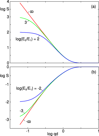
Figure 3. The logarithm of the surface response function S as a function of the logarithm of qd, where q is the wavevector and d the film thickness, for two different cases: (a) stiff layer on top of a soft semi-infinite solid and (b) soft layer on top of a semi-infinite stiff solid. The red curves are results for (a) a free elastic slab and (b) an elastic slab on top of a rigid solid. In both cases the Poisson ratio ν0 = ν1 = 0.5.
Download figure:
Standard imageNote that bending effects are fully taken into account in the theory presented above, since the derivation is based on the Navier equation of motion of an elastic body, which is the foundation of the theory of elasticity and therefore of also, in particular, for the theory of the bending of plates. As an example if one considers a free elastic plate described by equation (77) it is clear that for small values of qd one exactly gets the solution for pure bending of plates. Thus if we assume qd ≪ 1 and expand both the numerator and denominator in (77) to leading order in qd we get Sa = 6/(qd)3. Substituting this into the definition Mzz =− 2S(q)/(E*q) gives Mzz =− 12/(E*q4d3). This is exactly the result obtained from the theory of the bending of plates, where the normal displacement u satisfies D∇2∇2u =− σ or, after Fourier transformation, u(q) =− σ(q)/(Dq4), where the bending stiffness D = E*d3/12. This is identical to the prediction of (77) for qd ≪ 1.
5. Numerical results
In what follows we will present numerical results for two surfaces a and b, with the power spectra shown in figure 4. Both surfaces have the root-mean-square roughness 10 µm and the large and small wavevector cutoff q1 = 3.9 × 10¹⁰ m−1 and q0 = 103 m−1. Curve b is with the roll-off wavevector qr = 105 m−1 while in case a there is no roll-off. For qr < q < q1 the surfaces are self-affine fractal with the fractal dimension Df = 2.2 (corresponding to the Hurst exponent H = 0.8). Note that the rms roughness hrms is mainly determined by the longest wavelength roughness, while the area of real contact is determined mainly by the short-wavelength roughness. It is interesting to note that, for q > qr, the power spectra C(q) for surface b is ∼1000 times larger than for surface a, in spite of the fact that the two surfaces have the same rms roughness value. This has important implications for the leak rate of seals (see below).

Figure 4. The logarithm of the surface roughness power spectrum C as a function of the logarithm of the wavevector q for two surfaces with the root-mean-square roughness 10 µm and the large and small wavevector cutoff q1 = 3.9 × 10¹⁰ m−1 and q0 = 103 m−1. Curve b is with the roll-off wavevector qr = 105 m−1 while in case a there is no roll-off. For qr < q < q1 the surface is self-affine fractal with the fractal dimension Df = 2.2 (corresponding to the Hurst exponent H = 0.8).
Download figure:
Standard image5.1. Contact area
In figure 5 we show for surface b the logarithm (with 10 as the base) of the (normalized) contact area as a function of the logarithm of the magnification. Figure 5(a) is for a d = 10 µm thick rubber film (elastic modulus E0 = 106 Pa, Poisson ratio ν0 = 0.5) on top of a stiffer semi-infinite solid (elastic modulus E1 = 109 Pa, Poisson ratio ν1 = 0.5), which we will refer to as Teflon, and (b) for the reversed system with Teflon film on rubber. The vertical dashed line indicates the magnification where q = ζq0 = 1/d. Also shown in the figure is the result obtained with only rubber (blue curve) and only Teflon (green curve). Note that for large magnification the contact area is given by the properties of the top layer. In what follows we will focus on case (b) with Teflon film on rubber. Real Teflon has similar elastic properties as we use above but a rather small penetration hardness (about 30 MPa) and will yield plastically already at rather low contact stresses. However, as we will argue below, this does not affect the leak rate of Teflon-coated rubber seals (see section 5.2) and we will neglect plastic yielding in most of the calculations in order to more clearly exhibit the basic physics involved in the contact mechanics for laminated systems.
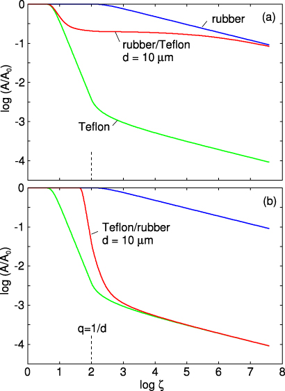
Figure 5. The logarithm (with 10 as the base) of the (normalized) contact area as a function of the logarithm of the magnification for (a) a d = 10 μm thick rubber film (elastic modulus E0 = 106 Pa, Poisson ratio ν0 = 0.5) on top of a semi-infinite Teflon solid (elastic modulus E1 = 109 Pa, Poisson ratio ν1 = 0.5) and (b) for the reversed system Teflon on rubber. The squeezing pressure p = 1 MPa and the surface roughness power spectra given by curve b in figure 4.
Download figure:
Standard imageIn figure 6 we show the logarithm (with 10 as the base) of the (normalized) contact area as a function of the logarithm of the magnification for a d = 10 μm thick Teflon film on top of a semi-infinite rubber solid. The two curves are for the two power spectra a and b in figure 4. The leak rate is determined mainly by the size of the critical junction observed (during increasing magnification) at the magnification ζc, where the first percolating channel appears, i.e. for A(ζc)/A0 ≈ 0.5. At the squeezing pressure used in figure 6 (p = 1 MPa) we get ζc ≈ 70 and ≈100 for surfaces b and a, respectively. This correspond to the wavevectors q = ζcq0 ≈7× 10⁴ and ≈105 m−1. Figure 4 shows that for these wavevectors the surface roughness power spectrum is much larger for surface b than for surface a, and we therefore expect larger leakage for surface b.

Figure 6. The logarithm (with 10 as the base) of the (normalized) contact area as a function of the logarithm of the magnification for a d = 10 μm thick Teflon film (elastic modulus E1 = 109 Pa, Poisson ratio ν1 = 0.5) on top of a semi-infinite rubber solid (elastic modulus E0 = 106 Pa, Poisson ratio ν0 = 0.5). The two curves a and b are for the two power spectra a and b in figure 4. The squeezing pressure p = 1 MPa.
Download figure:
Standard imageTeflon has a Poisson ratio ν ≈ 0.5 and polymers in general have 0.3 < ν < 0.5. In figure 7 we show the logarithm (with 10 as the base) of the (normalized) contact area as a function of the logarithm of the magnification for two d = 10 μm thick polymer films with the elastic modulus E1 = 109 Pa and the Poisson ratio ν1 = 0.5 and 0.3, on top of a semi-infinite rubber solid. In both cases we have assumed the power spectra b in figure 4. Note that the contact area depends only weakly on the Poisson ratio.
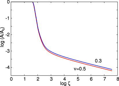
Figure 7. The logarithm (with 10 as the base) of the (normalized) contact area as a function of the logarithm of the magnification for two d = 10 μm thick polymer films with the elastic modulus E1 = 109 Pa and the Poisson ratio ν1 = 0.5 and 0.3, on top of a semi-infinite rubber solid (elastic modulus E0 = 106 Pa, Poisson ratio ν0 = 0.5). The curves are for the power spectra b in figure 4. The squeezing pressure p = 1 MPa.
Download figure:
Standard imageFigure 8 shows the logarithm of the (normalized) contact area as a function of the logarithm of the magnification for two d = 10 μm thick polymer films with the elastic modulus E1 = 109 Pa and the Poisson ratio ν1 = 0.5, on top of a semi-infinite rubber solid (elastic modulus E0 = 106 Pa, Poisson ratio ν0 = 0.5). The dashed curve is for elastic contact (from figure 6), while the blue and green curves are for elastoplastic contact with the penetration hardness 30 MPa as is typical for Teflon. The blue curve is the contact area which has yielded plastically and the green curve the elastic contact area. The curves are for the power spectra a in figure 4.
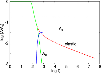
Figure 8. The logarithm (with 10 as the base) of the (normalized) contact area as a function of the logarithm of the magnification for two d = 10 µm thick polymer films with the elastic modulus E1 = 109 Pa and the Poisson ratio ν1 = 0.5, on top of a semi-infinite rubber solid (elastic modulus E0 = 106 Pa, Poisson ratio ν0 = 0.5). The dashed curve is for elastic contact (from figure 6), while the blue and green curves are for elastoplastic contact with the penetration hardness 30 MPa. The blue curve is the contact area which has yielded plastically and the green curve the elastic contact area. The horizontal dotted line corresponds to A/A0 = 0.5. The curves are for the power spectra a in figure 4. The squeezing pressure p = 1 MPa.
Download figure:
Standard imageThe horizontal dotted line in figure 8 correspond to A/A0 = 0.5. The condition A(ζ)/A0 ≈ 0.5 determines the point where the non-contact percolates which results in most of the leak rate of seals (see section 5.2). Note that at the magnification when the contact area equals A/A0 = 0.5 plastic deformation is negligible. Thus we can neglect plastic deformation when studying the leak rate for surface a squeezed against a flat surface at the (nominal) contact pressure 1 MPa, which is typical for rubber seals.
5.2. Leak rate for laminated rubber seals
Rubber seals, e.g. rubber O-rings, is of great importance in very many mechanical constructions. Because of its low elastic modulus (E ≈ 1 MPa), already nominal contact pressures of order ∼1 MPa may result in nearly complete contact between a rubber body and the countersurface, e.g. a polished steel surface, resulting in good sealing. However, the friction between the rubber and an unlubricated countersurface can be very high, e.g. the friction coefficient for a rubber–steel contact is typically of order unity, and sometimes even higher. In some applications the confined fluid has a very low viscosity, e.g. for water, and in this case the friction may be very high for all relevant sliding velocities. In such cases it may be useful to coat the rubber surface with a low friction material like Teflon. However, Teflon, and other coating materials, usually have a much higher elastic modulus than rubber which may result in large non-contact (fluid leak) channels at the interface for laminated rubber seals. Here we will show how the theory developed above may be used to study this problem in detail.
In earlier publications we have studied fluid flow at interfaces using the so-called critical junction theory and an effective medium theory [16, 17]. The critical junction theory is accurate at high enough contact pressures, while the effective medium theory holds (approximately) for all contact pressures. Let us first briefly describe the critical junction theory.
Consider the fluid leakage through a rubber seal, from a high fluid pressure Pa region, to a low fluid pressure Pb region. Assume for simplicity that the nominal contact region between the rubber and the hard countersurface is rectangular with area L × L. Now, let us study the contact between the two solids as we change the magnification ζ. We define ζ = L/λ, where λ is the resolution. We study how the apparent contact area, A(ζ), between the two solids depends on the magnification ζ. At the lowest magnification we cannot observe any surface roughness and the contact between the solids appears to be complete i.e. A(1) = A0. As we increase the magnification we will observe some interfacial roughness and the (apparent) contact area will decrease. At high enough magnification, say ζ = ζc, a percolating path of non-contact area will be observed for the first time. The most narrow constriction along the percolation path, which we denote as the critical constriction, will have the lateral size λc = L/ζc and the surface separation at this point is denoted by uc = u1(ζc), and is given by the Persson contact mechanics theory. As we continue to increase the magnification we will find more percolating channels between the surfaces, but these will have more narrow constrictions than the first channel which appears at ζ = ζc, and as a first approximation we will neglect the contribution to the leak rate from these channels.
In the critical junction theory the leak rate is obtained by assuming that all the leakage occurs through the critical percolation channel and that the whole pressure drop ΔP = Pa − Pb occurs over the critical constriction (of length (in the fluid flow direction) λx and width λy, with λx = λy = λc ≈ L/ζc and height uc = u1(ζc)). Thus, for an incompressible Newtonian fluid, the volume-flow per unit time through the critical constriction will be (Poiseuille flow)
where η is the fluid viscosity. For a rectangular nominal rubber-countersurface there is an additional factor Ly/Lx in (79), where Lx is the length (in the direction of fluid flow) and Ly is the width of the nominal contact region. Typically Ly/Lx ≫ 1.
To complete the theory we must calculate the separation uc of the surfaces at the critical constriction. We first determine the critical magnification ζc by assuming that the apparent relative contact area at this point (where the non-contact area percolates) is given by the Bruggeman effective medium theory: A(ζc)/A0 = 0.5. Knowing the critical magnification ζc, the separation uc = u1(ζc) at the critical junction can be obtained using the Persson contact mechanics theory.
The leak rate can also be expressed in terms of the flow factor ϕp. First note that the ensemble averaged current in the x direction  or since
  we get the leak rate
Thus, ϕp can be determined from the leak rate  if the average surface separation
  is known. In the calculations presented below we have used the effective medium theory for the leak rate of seals. For high squeezing pressures this latter theory gives almost the same result as the critical junction theory [18], but for small contact pressures the effective medium theory is more accurate, and in fact for very small contact pressures it gives the same result for
  (where
  is the average interfacial separation) as predicted by the Tripp theory (which is exact to order
  ).
).
Figure 9 shows the logarithm (with 10 as the base) of the leak rate as a function of the logarithm of the squeezing pressured for a d = 10 μm thick Teflon film on top of a semi-infinite rubber block. The results are again for the power spectra a and b in figure 4 and for the (Teflon) laminated rubber (solid lines) and for pure rubber (dashed lines). The fluid viscosity η = 0.001 Pa s, the fluid pressure drop ΔP = 0.1 MPa and the ratio Lx/Ly = 16. Note that the Teflon film for most squeezing pressures increases the leak rate by many orders of magnitude. Note also that, as the squeezing pressure goes toward zero, the leak rate for the laminated and pure rubber seals approach each other, which is expected because for low contact pressure the long-wavelength λ roughness will determine the leak rate and the contact mechanics at large length scales (λ ≫ d) is not dependent on the stiff coating.

Figure 9. The logarithm (with 10 as the base) of the leak rate as a function of the logarithm of the squeezing pressure for a d = 10 μm thick Teflon film (elastic modulus E1 = 109 Pa, Poisson ratio ν1 = 0.5) on top of a semi-infinite rubber solid (elastic modulus E0 = 106 Pa, Poisson ratio ν0 = 0.5). The results are for the power spectra a and b in figure 4 and for the (Teflon) laminated rubber (solid lines) and for pure rubber (dashed lines). The fluid viscosity η = 0.001 Pa s and the fluid pressure drop ΔP = 0.1 MPa. We have assumed the ratio Lx/Ly = 16.
Download figure:
Standard imageThe fluid flow factor  for homogeneous bodies with isotropic surface roughness is a monotonically increasing function of
  . However, this is not always the case for layered materials. Thus, in figure 10 we show the pressure flow factor ϕp as a function of the average interfacial separation for a d = 10 μm thick Teflon film on top of a semi-infinite rubber block. The results are for the power spectra a and b in figure 4. The origin of the non-monotonic dependence of
  on
on  for surface a can be understood as follows.

Figure 10. The pressure flow factor ϕp as a function of the average interfacial separation for a d = 10 μm thick Teflon film (elastic modulus E1 = 109 Pa, Poisson ratio ν1 = 0.5) on top of a semi-infinite rubber block (elastic modulus E0 = 106 Pa, Poisson ratio ν0 = 0.5). The results are for the power spectra a and b in figure 4.
Download figure:
Standard imageFor very large separation  (or low nominal contact pressures) the long-wavelength roughness will determine the flow factor and, with respect to the long-wavelength roughness, the layered material will deform as if the stiff top layer would not exist, and
  will increase with increasing
  as expected for a homogeneous solid with the bulk (rubber) elastic properties. Note that the rms roughness hrms is dominated by the long-wavelength contribution. As we increase the applied stress,
  will decrease and the elastic solid will deform and follow the long-wavelength roughness down to a point where the wavelength becomes of the order of the thickness of the Teflon coating. From here on the contact area and the interfacial separation is mainly determined by the Teflon film, but now the relevant surface roughness is only the wavelength component smaller than the thickness of the film. Thus, with respect to the contact mechanics for small
  the surface roughness
  appears much smaller than the full roughness hrms. This implies that for small
  the flow factor will increase with
  at a rate much higher than at large
  . This explains the general form of curve a in figure 10. For surface b there is almost no long-wavelength roughness and the flow factor (and leak rate) is determined mainly by the Teflon layer for all
  and this explains why the flow factor in this case takes its usual form, being a monotonically increasing function of
  .
.
To summarize, the fluid flow factor for a homogeneous and isotropic material is a monotonically increasing function u/hrms. In the case of layered materials, below a certain threshold of  the flow factor will be depend on the ratio
  and since
  is much smaller than hhrm this means that
  and therefore the flow factor will take almost the same value that it would take in the case of a homogeneous and isotropic material at much higher values of
  . This explains the non-monotonic behavior of the curve.
6. Summary and conclusion
We have applied the contact mechanics model of Persson to layered materials. We have derived the M function, which relates the surface stress to the surface displacement, for a layered material, where the top layer (thickness d) has different elastic properties than the semi-infinite solid below. The formalism is valid for viscoelastic solids but is applied in this paper only to elastic materials. We have presented numerical results for the contact area as a function of the magnification for several different cases. For small magnifications, where only the long-wavelength roughness is observed, the contact mechanics does not depend on the thin-film coating. For very large magnification the contact area is the same as if the coating film would be infinitely thick. The transition from bulk to surface film dominance occurs at the magnification where the roughness wavelength of the order of the thickness of the film can first be observed. We have also studied the dependence of the contact area on the Poisson ratio and plastic yield stress. We find that changing the Poisson ratio for the coating material from 0.5 (Teflon) to 0.3 (lower limit for polymer coatings) has a very small influence on the contact area. When plastic yielding is included in the analysis, the surfaces deform elastically with respect to the long-wavelength roughness (low magnification) but plastically at high enough magnification (involving shorter wavelength roughness).
As an application, we have studied the fluid leak rate for laminated rubber seals with Teflon-like coating. The large stiffness of the coating film as compared to the rubber bulk material underneath results in larger interfacial separation and larger leak rate as compared to the uncoated rubber seal. In most cases the critical junction, which determines most of the leakage, is observed at a magnification where negligible plastic deformation has occurred. As a result, in most cases it is not necessary to include plastic deformation when estimating the leak rate, even for coating materials like Teflon with a relatively low yield stress or penetration hardness. Finally, we have shown that for layered materials the fluid pressure flow factor ϕp may be a non-monotonic function of the average interfacial separation, in contrast to homogeneous materials with isotropic roughness for which ϕp increases monotonically with increasing  .
.
Acknowledgments
I thank G Carbone for useful discussions. This work, as part of the European Science Foundation EUROCORES Program FANAS, was supported from funds by the DFG and the EC Sixth Framework Program, under contract no. ERAS-CT-2003-980409.