
Abstract
Two different plasma actuation strategies for producing near-wall flow oscillations, namely the burst-modulation and beat-frequency mode, are characterized with planar particle image velocimetry in quiescent air. Both concepts are anticipated to work as non-mechanical surrogates of oscillating walls aimed at turbulent flow drag reduction, with the added benefit of no moving parts, as the fluid is purely manipulated by plasma-generated body forces. The current work builds upon established flow-control and proof-of-concept demonstrators, as such, delivering an in-depth characterization of cause and impact of the plasma-induced flow oscillations. Various operational parameter combinations (oscillation frequency, duty cycle and input body force) are investigated. A universal performance diagram that is valid for plasma-based oscillations, independent of the actuation concept is derived. Results show that selected combinations of body force application methods suffice to reproduce oscillating wall dynamics from experimental data. Accordingly, the outcomes of this work can be exploited to create enhanced actuation models for numerical simulations of plasma-induced flow oscillations, by considering the body force as a function of the oscillation phase. Furthermore, as an advantage over physically displaced walls, the exerted body force appears not to be hampered by resonances and therefore remains constant independent of the oscillation frequency. Hence, the effects of individual parameter changes on the plasma actuator performance and fluid response as well as strategies to avoid undesired effects can be determined.
Export citation and abstract BibTeX RIS

Original content from this work may be used under the terms of the Creative Commons Attribution 4.0 license. Any further distribution of this work must maintain attribution to the author(s) and the title of the work, journal citation and DOI.
1. Introduction
The development of plasma-based flow-control actuators has experienced a brief time span [1] nevertheless leading to a considerable variety of numerous electrical and mechanical characterisation studies. These have led to rapid advances in plasma actuator (PA) technology, as summarized in reviews in the past two decades [2–6].
In the branch of turbulent flow control different concepts and mechanisms, aimed at viscous drag reduction, have been developed so far [7]. A promising concept is streamwise traveling waves (StTWs) of spanwise wall velocity [8], which impart a periodic fluid oscillation transverse to the mean-flow direction and modulated along the streamwise direction. The key element is the generation of a so-called generalized Stokes layer [9], a near-wall shear layer that favourably modifies flow structures inherent to the viscous sublayer and consequently reduces friction drag [10–14]. The parameter space of StTWs spans a spectrum of temporal oscillation frequencies f and streamwise wavenumbers κx
[13], where the oscillation waveform has an additional effect on both drag control performance and efficiency [15]. For  , the StTWs become the limiting case of pure temporal oscillation of spanwise wall velocity [10, 12] which is the investigated mechanism of particular interest in the present work.
Formerly, complex control devices [11, 14], mechanical inertia [10] and resonant effects [12] have come in contradiction to the advantages of active flow-control (AFC) devices. By design, the simplicity and absence of moving parts make PAs very attractive candidates for a successful implementation of StTW. As one of the most common types, the alternate-current dielectric barrier discharge (AC-DBD) PA is known to mainly produce a volume-distributed body force along the wall-parallel direction that drives a quasi-steady wall jet [16–18]. Both magnitude and distribution of this body force are major key-quantities to determine the fluid-mechanical impact of an operative PA (thus flow-control performance). They can be determined using different types of numerical models [19–24], by direct integral measurements [16, 25, 26] or can be computed by using velocity-field information to estimate either the spatial force distribution [17–19] or the integral force magnitude [16, 17, 27–30]. A particularly supportive characteristic, in view of mimicking wall oscillations, is their fast response time allowing to rapidly switch the forcing direction and, consequently, to induce an oscillatory fluid motion near the wall [31–34]. These fluid-mechanic attributes and the structural properties of AC-DBD PAs render them also a relevant AFC candidate for turbulent flow manipulation.
In previous works [31, 35, 36] different approaches and concepts dedicated to unsteady excitation of plasma discharges have been investigated. The burst-modulation mode is one of such approaches that has been applied by Jukes et al [32] to generate spanwise flow oscillations in a turbulent boundary layer. They operated an intermittent array of three-electrode PAs and achieved drag reduction (≈45%), despite the remaining gaps between the individual PAs that led to inhomogeneities of the spanwise flow. Therefore, they suggested that a decrease of the spanwise forcing wavelength, ideally without any gaps, becomes more beneficial. This was initiated by Hehner et al [33] who developed and successfully tested a non-interrupted electrode configuration that reduces the aforementioned gaps [32] to a minimum, i.e. to the width of the exposed electrode. Accordingly, the forcing wavelength was halved. An alternative approach for discharge excitation, inspired by Wilkinson [31], is the beat-frequency mode that was adapted by Hehner et al [34] to be tested on the above-described continuous electrode configuration [33].
Compared to a classical wall-driven Stokes layer, plasma-based oscillations [32–34] have shown that wall-normal velocity components occur, due to unavoidable spanwise discontinuities in the body force topology. Additionally, for static walls obeying the no-slip condition, the maximum spanwise velocities have to develop above the wall. These distinguishable features notwithstanding, the very limited amount of experimental studies on this mode of plasma-enabled actuation has demonstrated promising advancements and further developments that encourage more investigations into the direction of turbulent flow control and of mimicking StTWs. In general, progress in PA understanding was made through several characterization studies of PAs, fostering the understanding of their working principle and promoting a systematic application to boundary-layer flows. Likewise, the lack of works on plasma-induced flow oscillations reveals the need for in-depth characterizations of flow-control [32] and proof-of-concept [33, 34] demonstrators, in order to gain particular insights into the actuation mechanisms.
The objective of the present work is hence to elucidate the attributes of plasma-induced flow oscillations based on two distinctively different excitation strategies, namely burst-modulation [33] (BM) and beat-frequency [34] (BF), and identify their parametric effects on the induced flow topology and performance. The experiments are carried out in quiescent-flow conditions and the parameter space accommodates a range of oscillation frequencies, duty cycles and input amplitudes. For the BF mode, however, the duty cycle is dependent on the input amplitude as will be explained in section 2.2. More specifically, the plasma-induced flow oscillations will be differentiated from the mechanically oscillating wall analogue by assessing the role of oscillation limiting factors (e.g. detrimental resonance effects [10, 12]), the produced waveforms [15], the flow homogeneity as a follow-up of the brief comparison made by Hehner et al [34] and the oscillation performance based on body-force input and fluid response. Furthermore, the inherent problems of estimating body-force distributions for plasma-based oscillations will be thoroughly discussed. As such, this work additionally attempts to provide accurate representation models of the PA system as input for numerical simulations that can support the definition of favorable control parameters to be applied retroactively under experimental conditions.
2. Dielectric-barrier discharge actuators and forcing strategies for near-wall oscillations
The hereby considered PA configurations of alternating staggered electrodes on the upper and lower side of the dielectric are shown in figure 1, each consisting of four individual electrode groups. Polyethylene terephthalate (PET) of 500 µm thickness was used as dielectric barrier and all electrodes were spray-painted with a conductive silver coating. The exposed and encapsulated electrodes have a width of 1 and 3 mm, respectively, and each a length of 100 mm. Hence, four wavelengths λz along the z direction (see figure 1) were covered, resulting in a total plasma length of 400 mm. An electrical insulation layer was applied to the encapsulated electrodes, preventing spurious discharges on the lower dielectric side. The z direction defined for this PA would be equivalent to the spanwise direction in a boundary-layer flow. Both contrasted concepts are briefly recapped below. Further information on the PA array and its operation modes can be found in the respective proof-of-concept studies of Hehner et al [33, 34].
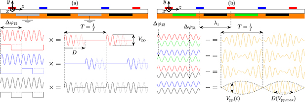
Figure 1. The considered concepts for oscillatory discharge actuation. Color-coded electrodes and high-voltage signals refer to HV1 (red), HV2 (blue), HV3 (black), HV4 (green) and ground (gray). The dielectric (white) and insulation layer (orange) are shown (not to scale). (a) Burst-modulation (BM) mode for 25% (and 50%, dotted lines) duty cycle. (b) Beat-frequency (BF) mode where the resulting high-voltage signals driving the discharge are displayed in yellow.
Download figure:
Standard image High-resolution image2.1. Burst-modulation (BM)
The BM mode is presented in figure 1(a) and shows that the exposed electrodes HV1 (red) and HV2 (blue) each obtain a high-voltage AC sine-wave signal that is multiplied by a square signal. The latter is the burst function with burst frequency  that triggers the plasma discharges. As one requirement for the oscillatory discharge, HV1 and HV2 receive the same burst functions with a phase shift of
  . On the lower dielectric side, another high-voltage electrode pair HV3 (black) and one grounded electrode pair (gray) complete this PA configuration. In order to maintain an oscillation of plasma discharges, HV3 is to be driven by a burst function of
  . As indicated by the dotted line in figure 1(a), HV3 is switched on at all times for duty cycles of 50%.
All high-voltage electrode groups, in this work, receive the same plasma-discharge frequency  kHz. The oscillation frequency f for the burst-modulation is determined by the burst frequency
  (see equation (1)).

For this particular triggering concept the duty cycle can be tuned independently from all other operational input parameters. The duty cycle should, however, be in the range  % for the present application. For D = 0 or D > 50% either no discharge or simultaneous discharges in opposing directions are produced, respectively. For the burst-modulation mode arbitrary combinations of oscillation frequency f, duty cycle D and input amplitude cover the testing parameter space.
2.2. Beat-frequency (BF)
The BF mode accomplishes a discharge oscillation without any grounded electrodes (i.e. fully floating potential) and the principle is shown in the schematic of figure 1(b). In contrast to the burst-modulation mode, the PA is connected to four independent high-voltage electrode groups: HV1 (red), HV2 (blue), HV3 (black) and HV4 (green). The discharge procedure underlies constructive and destructive interference of high-voltage AC sine-wave signals and, thus, it requires different plasma AC frequencies  (
( ) for the upper and lower electrodes. The difference in respective frequencies defines the resulting beat-frequency as
In general, this produces in-phase pulsating discharges between all electrodes. In order to achieve a periodic switching of the forcing direction, the AC signals of both upper and lower electrodes need a phase shift of a half period π, i.e.  . Hence, the oscillation frequency f becomes equal to the beat-frequency
  (see equation (3)).

The upper high-voltage electrodes HV1 and HV2 received  kHz and, accordingly, the lower electrodes HV3 and HV4 were provided with
  in order to enforce the desired settings for f. Therefore, the effective plasma-discharge frequency is
  .
.
The resulting differential voltage signals are shown as yellow lines in figure 1(b) and clarify that, in contrast to the burst-modulation mode, the peak-to-peak voltage  is a continuous function of time t. For the limiting case of π phase difference, the function is sinusoidal. This promptly involves a coupling of the effective duty cycle D and the maximum voltage amplitude (
 ) [34]. Specifically, the discharge onset is dictated by the breakdown field strength of the working medium, which in the present case is air at atmospheric conditions. Variation of
  , due to the sinusoidal envelopes (see figure 1(b), black dashed lines), implies that the breakdown field strength is exceeded or undercut at different positions within the phase of the beat cycle. Accordingly, the decrease of
  narrows the discharge period and reduces D, vice versa for the increase of
  . Therefore, the parameter space of the beat-frequency mode is reduced and can be decomposed into two independent parameters, namely the oscillation frequency f and the input amplitude. The duty cycle D, being directly affected by the input amplitude, is a dependent parameter.
3. Experimental procedure
3.1. Experimental setup and test cases
For the fluid-mechanical characterisation of the above-described concepts in section 2, time-resolved velocity information of the plasma-induced flow oscillations was acquired by means of planar high-speed particle image velocimetry (PIV). The coordinate system  is such that the x axis is parallel to the electrodes, y is the wall-normal coordinate and z refers to the (spanwise) forcing direction of the PA, which is across the electrodes (see figure 1). The velocity components u, v and w are aligned respectively to x, y and z directions. The flow was seeded with 1 µm di-ethyl-hexyl-sebacate (DEHS) particles (particle response time
  s, Stokes number Stk
  ) in a closed containment to ensure quiescent ambient conditions. The particles were illuminated via a wall-normal light sheet (
 -plane) at the PA-array center (x = 50 mm) by a Quantronix Darwin-Duo Nd:YLF laser. Two Photron FASTCAM SA4 cameras (active sensor size 1024 × 512 px2, 12 bits) equipped with Nikon Nikkor 200 mm lenses (
 ) with an additional flange focal distance of 70 mm were located perpendicularly to the light sheet, in order to capture two successive fields of view (FOV) with a 5 mm overlap and a spatial resolution of 80 px mm−1. The FOV was aligned with the dielectric surface and the merged images cover five exposed electrodes and respectively span four forcing wavelengths (
 mm). The control system for oscillatory PA operation is summarized in table 1. An ILA_5150 synchronizer control unit was used to coordinate double-cavity laser pulses, camera exposures and high-voltage transformers to run on a single clock.
Table 1. Overview of applied devices for the plasma control system.
| Device | Specifications | Classification |
|---|---|---|
| Function generator | Synchronizer control unit, | — |
| ILA_5150 GmbH | ||
| Power supply | VLP-2403 Pro | HV1 & HV2 |
| VSP-2410, | HV3 & HV4 a | |
| VOLTCRAFT® | ||
| High-voltage transformer | Minipuls 1 | HV1 |
| Minipuls 1 | HV2 | |
| Minipuls 2 | HV3 | |
| Minipuls 2, | HV4 a | |
| GBS Elektronik GmbH |
Images were acquired in double-frame mode with a pulse distance of  s. To ensure quasi-steady far-field conditions, the PA array was activated 10 s prior to the PIV measurement. In each test run the number of recorded oscillation cycles was locked at 225 with a phase resolution of 24 bins (
 ). Therefore, the camera frame rate
  was dependent on the selected oscillation frequency f in such a way that
  .
.
An overview of the conducted PIV experiments is shown in figure 2 as combinations of f and time-averaged electrical power consumption  for cases BM and BF. The corresponding frame rates
  of the cameras, to ensure the phase resolution of 24 image pairs per oscillation cycle, are added to the right ordinate of figure 2 for clarity. In addition, the underlying peak-to-peak voltages are added to the upper abscissa for completeness. The variation of D for case BM was performed at constant voltage amplitude, where a linear relation of D and
  [37] can be identified. The respective test cases are presented in figure 3, where the dashed lines further support the D-
 relation.
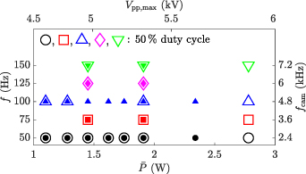
Figure 2. Map of the investigated parameter space for the PIV experiments: oscillation frequency f (~frame rate  ), peak-to-peak voltage
  and corresponding time-averaged electrical power consumption
  . Open and solid symbols refer to cases BM and BF, respectively.
Download figure:
Standard image High-resolution image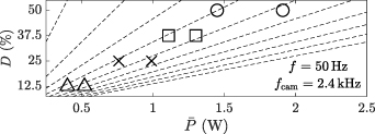
Figure 3. Additional D- parameter space of PIV experiments for case BM; the dashed lines indicate constant ratios of
  and D (
 [37]).
Download figure:
Standard image High-resolution imageThe time-averaged power consumption  and for case BM has been quantified on the grounds of the electrical treatise by Kriegseis et al [38], where also the corresponding electrical efficiency
  of the setup was determined [39]. The accordingly calibrated input power
  of the power supply subsequently guaranteed an actuator operation at identical constant power levels for the case BF—despite the absence of grounded electrodes and related implications for the power measurements [40].
3.2. Data processing and measurement uncertainty
For PIV processing, PIVTECs PIVview2C software (version 3.8.0) was used in a multi-grid approach, where the raw images were cross-correlated on a final interrogation window size of 16 × 8 px2 (z × y) with an overlap factor of 50%. As such, the resulting velocity information was derived with a spatial resolution of 10 and 20 vectors mm−1 in z and y direction, respectively. A normalized median test [41] (threshold 2.5) was used to replace 3.5% outliers with the second highest correlation peak. Further post-processing of the velocity information and combination of the two FOVs was done on Matlab.
A random velocity field of the merged FOVs is shown in figure 4 to indicate the processing approaches. The convergence of the PIV data was checked by computing the relative standard deviation [17, 42]  of the horizontal velocity component w. The standard deviation
  alone considers both true velocity fluctuations and measurement errors (
 ) [43]. The relative standard deviation is shown in figure 5(a) at specific locations of the velocity field, being depicted in figure 4 by the black symbols. The amount of recordings per wavelength was
  and this number was increased to
  by taking all four captured wavelengths into account. It is obvious that the data has significantly converged for N > 200. The convergence of the PIV data at the wall-jet location (
 ) is additionally indicated by the color-coded diamonds for single λz
(
) is additionally indicated by the color-coded diamonds for single λz
( ). In this region,
  was found for all PIV experiments of cases BM and BF, whereas
  is found for single λz
. Despite the phase-locked observation of a periodic process, a slightly larger relative standard deviation than typically found in literature for a quasi-steady PA-based wall jet [17] is obtained.
is found for single λz
. Despite the phase-locked observation of a periodic process, a slightly larger relative standard deviation than typically found in literature for a quasi-steady PA-based wall jet [17] is obtained.

Figure 4. Illustration of the post-processing strategies. Velocity vectors of phase-resolved velocity field in the y, z-plane are shown. The orange solid line (at y ≈ 0.25 mm) indicates the integration domain of equation (8). The purple rectangles depict the control volumes and surfaces of equation (5). The top boundary of the control volumes is at y = 0.9 mm. Exposed and encapsulated electrodes are added in light and dark gray, respectively. Symbols and color fill indicate locations for the convergence studies. Velocity profiles are evaluated along the green dashed lines.
Download figure:
Standard image High-resolution image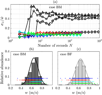
Figure 5. (a) Typical PIV-convergence diagram at different flow-field locations (see figure 4). (b) PDF of w at the wall-jet location. Color-coded symbols in (a) and dots in (b) refer to the same single λz
. The color code is indicated in figure 4 to be related to the respective  location.
Download figure:
Standard image High-resolution imageSuch deviations can be expected as the fluid undergoes a complete reversal of motion during one oscillation cycle, where small uncertainties in the supplied driving signal can already produce large fluctuations. Another sensitive aspect is the fine tuning of the high-voltage transformers, in order to minimize differences between the discharges intensities of all four λz and, as such, to generate volume body forces of equal strength. This effect can lead to the higher relative standard deviation as observed in figure 5(a) for N = 900 and is therefore visualized in the probability density functions (PDF) in figures 5(b) and (c). The color-coded dots each belong to the same data shown in figure 5(a) for single λz . The comparison of cases BM and BF shows that for case BM one of the discharges can deviate from the others, whereas for case BF the fluctuations around the mean values are larger. The latter can be identified smaller for case BM, while the mean values for single λz of case BF appear identical due to the coupled character of the respective HV-devices for this operating mode.
The measurement uncertainty of the PIV-correlated velocity components was additionally estimated by applying the correlation-statistics method presented by Wieneke [44] and Sciacchitano et al [45]. This method uses the PIV raw images and displacement fields, in order to dewarp the cross-correlated interrogation windows of the second frame back onto the first frame. The uncertainty field is then computed from intensity differences in each interrogation window and it represents the approximate measurement errors  of the velocity components [43]. Accordingly, the absolute error averaged for a single displacement field was determined as
  px (or 0.03 m s−1) and
  px (or approx.
  ).
).
4. Post-processing strategy
4.1. Body-force magnitude estimation
The volume-distributed body force emerges as a result of the fast collisional processes between charged and neutral species and is the main mechanism driving the resultant induced flow topology by the PA. As such, it is an important benchmark for the PA performance that can be quantified and analysed by inserting the acquired velocity information into differential [16–19, 46], integral [16, 27–29] or hybrid [30] forms of the Navier–Stokes momentum equation.
Insights into the spatial body-force distribution can be gained from the differential approaches. However, the existence of the unknown pressure field renders the problem underdetermined, when only velocity information is used. For a quasi-steady wall jet in quiescent-air surroundings, a closing assumption must be made, usually considering that the body force prevails over the pressure gradient and hence it can be neglected [47]. This assumption, however, is an oversimplification for heavily unsteady flow, as was demonstrated for the initial stages of the actuation when a starting vortex is formed that typically requires  ms to be washed out and to reach quasi-steady conditions for the PA [16]. Another, simpler approach that bypasses the previous assumption is the so-called 'reduced method', as introduced by Kotsonis et al [16]. The reduced method accounts only for the acceleration term of the momentum balance via
  , which is assessed in the very first moments after actuation. In this state the contribution of all other terms can be shown to be small and can be neglected from the momentum balance. As a result, the force magnitude Fj
is underestimated by about 20%, when compared to performing the force evaluation on the quasi-steady wall jet [16].
, which is assessed in the very first moments after actuation. In this state the contribution of all other terms can be shown to be small and can be neglected from the momentum balance. As a result, the force magnitude Fj
is underestimated by about 20%, when compared to performing the force evaluation on the quasi-steady wall jet [16].
The momentum balance in integral form writes
which yields the body-force magnitude as an additional source term Fj , albeit no spatial information can be gained. For the wall jet, the common quasi-steady assumption is made, justifying the negligence of the unsteady term in equation (4) (see e.g. Versailles et al [29]). The force is then obtained by evaluating both the momentum fluxes across the surface S and the shear stress at the wall. The pressure is assumed uniform for the control-volume borders chosen far enough from the bulk of the plasma-induced force. In the work of Debien et al [30] it was shown that concise temporal variations of the body force—present during one plasma discharge cycle—can be accounted for, when the unsteady term in equation (4) is additionally evaluated.
The PA described in section 2 drives periodically oscillating body forces to induce a near-wall flow oscillation. The resulting flow topology for this PA configuration is established from Hehner et al [34] who showed the two-dimensional velocity fields  of two oppositely arranged phase positions within an oscillation cycle for case BF. A representative field is shown in figure 4. For the oscillation periods
  of the current PIV data set
  ms holds (cp. figure 2) and therefore the quasi-steady state is not reached as also confirmed by the earlier proof-of-concept study by Hehner et al [34] who operated the PA with f = 50 Hz (or T = 20 ms). Therefore, for the unsteady plasma-induced flow oscillations, the time-dependent term has to be accounted for, in order to resolve the time-dependent body force at each phase position of the oscillation cycle. Furthermore, as the presence of the starting vortex involves an unknown local pressure gradient that cannot be neglected, the common differential approach [18] cannot be applied. Last but not least, for the case of continuously operated plasma flow oscillations, as the flow field of continuously operated plasma flow oscillations does not come to rest, the sole application of the reduced method (corresponding to the first term in equation (4)), is also prohibitive due to the absence of the required quiescent-air environment prior to the actuation.
Considering the limitations of the aforementioned body-force estimation techniques, the unsteady integral (hybrid) form of the momentum balance [30] as given by equation (4) is applied in the present work—interpreted as a combination of the methods of Kotsonis et al [16] and Versailles et al [29]. The chosen control volume (CV) is a box that encloses one wavelength λz of the PA. This choice ensures that the CV borders have sufficient distance from the plasma bulk [16] and allow dropping the pressure term in equation (4). The four selected control volumes are highlighted in figure 4 by the magenta boxes. Each of them considers one λz and was individually evaluated along the surfaces S1, S2, S3 and S4. Afterwards, the average of four λz was computed. As stated in earlier studies [16, 17, 30], the wall-normal force component Fy is an order of magnitude smaller than the wall-parallel force component Fz . Accordingly, the total actuator force Fz is be computed, explicitly rewriting equation (4) to
where the wall shear stress  is
is
The first right-hand side term in equation (5) includes the rate of change of the spanwise flow component  that has been approximated for all acquired phase positions ϕm
(
that has been approximated for all acquired phase positions ϕm
( ) via central differences [48]
where the time lag between phases  and
and  or the phase-to-phase spacing
  is dependent on f.
It is further important to note that the total actuator force [17] has to be distinguished from the net force [16, 28], known as thrust, as it disregards the shear forces at the wall. The uncertainty of the force component Fz
, resulting from equation (5), was evaluated based on the relative standard deviation of the velocity  . The computation of Fz
was repeated, by inserting
. The computation of Fz
was repeated, by inserting  into the flux terms (across S2, S3, S4) of equation (5), resulting in a deviation of
  for single λz
and of
for single λz
and of  for the spatial mean of all four λz
.
for the spatial mean of all four λz
.
4.2. Amplitude of the virtual wall oscillation
The second relevant performance measure is obtained from the fluid response to the exerted body force. For turbulent flow control, the amplitude of physically realizable spanwise-oscillating walls is crucial, affecting both the amount of drag reduction and required power (i.e. efficiency of the control) [13]. In such case, the resulting flow field is one-dimensional (w(y) and  ) in space (along y) and the temporal oscillation can be described by analytical solutions of the first Stokes problem. The use of PAs on non-moving walls to generate flow oscillations implies, however, zero fluid velocity at the wall due to the no-slip condition. This was confirmed in the studies by Hehner et al [33, 34] who showed the resulting velocity profiles w(y) of the induced oscillation at different locations along the z direction. Accordingly, the maximum velocity was found slightly above the wall surface, which nonetheless revealed a Stokes-layer-like flow behavior for
  .
.
However, as a consequence of the discharge discontinuity at the exposed electrode (see also figure 1), the PA produces a two-dimensional flow in the z direction that varies periodically at the wavelength λz
as evident from figure 4. Consequently, the integrated effect of the horizontal flow component  may be considered a meaningful performance metric. For the remainder of this work, this will be defined as the 'virtual wall velocity'
where n is the number of wavelengths (here n = 4, see figure 4) and  is the phase-resolved horizontal velocity component. The virtual wall velocity
  enables both, a comparison to the analytical Stokes-layer solution and the quantification of the inherent cause-effect relations between exerted body force and resulting flow fields. As illustrated in figure 4, the integral in equation (8) is computed along the orange solid line at
  (at y ≈ 0.25 mm) as an equivalent to the oscillating wall that exhibits the maximum velocity at the wall. Gatti et al [12] defined the oscillating-wall amplitude as the maximum oscillation velocity, which accordingly corresponds to the maximum value of the virtual wall velocity
  in the present context.
A more rigorous evaluation measure is  , which is the time mean of
  , thus compensating for the fluid being periodically accelerated and decelerated during an oscillation cycle. Note that for an oscillating wall this would similarly be the ratio of peak-to-peak displacement of the wall (analogous to the stroke) and half oscillation period (
 ).
).
5. Results and discussion
5.1. Fluid response
The induced flow topology of the plasma-induced flow oscillations of both concepts have already been elaborated by Hehner et al [33, 34], where figure 4 demonstrates the repeatability between the former experiments and the present study. The focus in this section is on a comparison of the temporal and spatial shape of the produced oscillation waveforms to the analytical solution of the first Stokes problem.
The time-dependent fluid response of the oscillating plasma discharges for cases BM and BF is compared in figure 6 by means of the phase-resolved virtual wall velocities  ; see equation (8). All curves show the produced oscillation waveforms with respect to D, f and the excitation concept. The (sinusoidal) Stokes-layer waveform is additionally added to each graph as a reference.
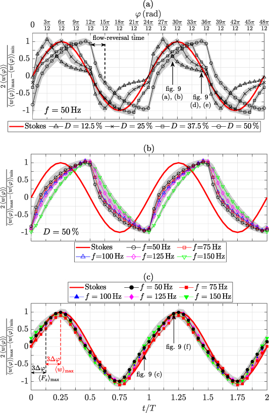
Figure 6. Comparison of normalized oscillation waveforms for cases BM and BF. (a) Case BM for  (f = 50 Hz). (b) and (c) Cases BM (D = 50%) and BF, respectively, for
  Hz. The red curves depict the Stokes-layer profile. The gray shadings correspond to standard deviation of experiments of constant f. The data is normalized between −1 and 1.
Download figure:
Standard image High-resolution imageIn figure 6(a) the normalized waveforms of case BM are plotted for variable D, showing the acceleration of the fluid during the actuated fraction of the duty-cycle period. Therefore, for D = 12.5% the fluid accelerates up to  , decelerating until the end of the half period (
 ) and then being accelerated along the other direction. Upon duty-cycle onset, the flow is instantly accelerated—independent from D, which leads to a faster velocity rise for lower D due to the longer relaxation time from the previous burst event in opposite direction. For D = 50%, in contrast, the flow reversal is retarded by
  , until counter-directed velocities occur, since the flow encounters a sudden sign flip of the forcing direction and accordingly has to decelerate from full speed; see figure 6(a). This observation is, therefore, considered disadvantageous in terms of an efficient transformation of body force into momentum. For
  % the flow is already immediately reversed. A comparison of the waveforms to the Stokes-layer profile (red curve) reveal agreement for D = 25% on the rising velocity branch, only, whereas the produced waveform for the burst-modulation mode is a distinguishing feature.
This waveform characteristic is also shown in figure 6(b) for all considered f at D = 50%. The waveform is weakly dependent on f, depicting a systematic decrease of the curve bending for larger f that can be explained as follows. The development time of the induced flow is shorter for larger f, therefore, the relative velocity increase is larger (steeper slope), whereas the phase-to-phase spacing is smaller.
The oscillation waveforms for case BF are presented in figure 6(c), where the waves are temporally aligned such as to have zero velocity at  . In fact, all curves coincide independent of f and they depict sinusoidal waveforms, endorsed by the outstanding agreement with the Stokes-layer profile.
The discharge excitation on the basis of time-dependent  has shown to transform into a continuous fluid response that forms a sinusoidal wave, similar to the Stokes-layer oscillation. In contrast, for case BM the integrated effect of the forcing is discontinuous. The discharge is abruptly triggered and the inherently impulsive burst brings about a strong impact on the surrounding fluid, producing large velocity gradients in the beginning of each half oscillation period. As such, case BM renders an alternative oscillation waveform, where the waveform character can additionally be controlled by the duty cycle.
For a further comparison of the fluid response and the analytical Stokes-layer solution the wall-normal root-mean-square (rms) profiles  of both plasma-induced flow oscillations and real Stokes layer were computed along the 24 resolved phases of the oscillations cycle, as shown in figure 7. The z location of the profiles corresponds to the center of the encapsulated electrodes
  , 1.5, 2.5 and 3.5 (see green dashed lines in figure 4). At this location the similarity of the velocity profiles to the analytical Stokes layer was found to be strongest (see e.g. Hehner et al [34]). For the shown fluctuation profiles all four individual profiles were averaged and normalized with the maximum velocity
  .
.
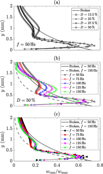
Figure 7. Comparison of root-mean-square profiles  for cases BM and BF. (a) Case BM for
  (f = 50 Hz). (b) and (c) Cases BM (D = 50%) and BF, respectively, for
  Hz. The gray curves depict the
  of the Stokes layer. The data is normalized by
  .
.
Download figure:
Standard image High-resolution imageIn figure 7(a) the rms profiles for different D (f = 50 Hz) are compared. It can be observed that a reduction in D leads to a reduction of the peak velocity fluctuations (y ≈ 0.25 mm) and to improved similarity with respect to the Stokes-layer profile, culminating in  . In particular, in the near-wall region (y ≈ 0.25 mm) and in the upper region (y > 1 mm) a good compliance is found. The effect of f for case BM is considered in figure 7(b), where in addition to the 50 Hz Stokes-layer rms profile the one for f = 150,Hz is also included. In compliance to a decrease of the rms value of the Stokes profile (with increasing f), the peak velocity fluctuations of the plasma-induced flow oscillations also decrease. However, the differences with respect to the Stokes layer increase significantly in the region of
  mm, which is dominated by the local minimum, inherent to the inversion of the body force direction. In this respect, for the fluctuation profiles of case BF in figure 7(c), both peak velocity fluctuations in the near-wall region (y ≈ 0.25 mm) and in the upper region (
 mm) show an improved fit, which can be attributed to the continuous flow-phase relationship, in contrast to the impulsive inversion inherent to the BM mode (see figure 6(c)).
Of particular interest is the difference of peak-velocity fluctuations of cases BM and BF that can be again attributed to the nature of the excitation concept. For case BM that is characterized by impulsive strokes on the fluid to reverse the flow, the fluctuations are larger. Instead, the smaller fluctuations of case BF immediately show the effect of a smoother transition of the flow from one to the other direction.
The deviations of the plasma-induced flow fluctuation profiles and the Stokes layer were further quantified by a mean-square error (MSQ) analysis. Accordingly, the squared deviations of the plasma-induced flow fluctuation profiles and the Stokes layer were computed and averaged along the wall-normal (y) direction. In figure 8(a) the error for variable D is shown. As already expected from figure 7(a), the error is smaller for  and the best fit to the Stokes solution is likely to be achieved in that range. Considering the variation of f in figure 8(b), the results clearly indicate that the similarity to the Stokes profile deteriorates for case BM with increasing f, while for case BF the error decreases slightly and remains about constant for
  Hz.
Hz.
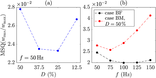
Figure 8. Mean-square error (MSQ) of the root-mean-square profiles of  in figure 7 with respect to the analytical solution of the Stokes layer. (a) Cases BM (f = 50 Hz). (b) Cases BM (D = 50%) and BF.
Download figure:
Standard image High-resolution imageThe features observed in figure 7 in combination to the MSQ error in figure 8 are in excellent agreement with the observations of the oscillation waveforms in figure 6. As in this section only integrated effects of the fluid response and velocity fluctuations at a certain position were considered, the flow homogeneity for the operation modes will be discussed in the following section.
5.2. Flow homogeneity
The developing flow field produced by plasma-based oscillations is two dimensional, where the horizontal flow is attenuated towards the exposed electrodes and a vertical flow component occurs to supply the actuation region with the required mass (see figure 4). These effects are visualised in figure 9 by means of phase-resolved vorticity fields and superposed velocity vectors for f = 50 Hz for similar power consumption. The phase positions shown in figure 9 were chosen according to the fluid responses and are indicated in figures 6(a) and (c). The phase positions considered in figures 9(a) and (d) refer to  and
and  , respectively, of case BM, D = 25%. Accordingly, for case BM, D = 50%, the phase positions refer to
  and
and  , as shown in figures 9(b) and (e), respectively. The vorticity for case BF is plotted in figures 9(c) and (f) in the same phase positions as for case BM, D = 50%.

Figure 9. Phase-resolved vorticity fields  for f = 50 Hz and
  W. (a) and (d) Case BM, D = 25% normalized by maximum value of all fields. (b) and (e) Case BM, D = 50%. (c) and (f) Case BF. Isolines (black dashed, solid and white) of λ2 [52] are displayed to aid identification of vortical structures. The phase positions of (a)–(c) and (d)–(f) are indicated in figures 6(a) and (c). Color levels from −0.5 to 1 s−1 (blue to red). Velocity vectors are added in gray.
Download figure:
Standard image High-resolution imageIn figure 9(a) a horizontal shear layer along the z direction has developed near the surface and a vortex has formed above. For case BM, D = 50% (figure 9(b)) this shear layer and corresponding vortex are weaker. This diminishing effect is even more pronounced for case BF (see figure 9(c)). As observed in 6(a) for D = 25% the flow was immediately reversed after switching the forcing direction, therefore, building up a spanwise shear layer. This is not the case for D = 50%, where the flow reversal is retarded, taking more time for the spanwise shear layer to develop. For case BF the fluid response was found to be continuous (see figure 6(c)), supporting the even weaker vortical structures compared to case BM, D = 50%. Both in figures 9(a) and (c) the spanwise shear layer appears to remain more attached to the wall, whereas in figure 9(b) it bends around the vortex. It must be noted here that upstream of the exposed electrodes for D = 25%, there are small recirculation zones which can occasionally occur in quiescent air conditions [49–51]. Their existence, however, becomes more unlikely for small ratios of exposed-to-encapsulated electrode widths [50] ( ; here:
  ).
).
At the later stage of the oscillation cycle (figures 9(d)–(f)) the horizontal shear layers have extended along the z direction for cases BM, D = 50% and BF. Comparing the two, the bending of the shear layer is more significant for case BM, which confirms the findings of Hehner et al [34] who concluded that for case BF the lift-up effect is slightly weakened. They showed this effect by analysing the wall-normal velocity profiles at different locations of λz . Furthermore, the shear layer covers about the entire discharge region (above the encapsulated electrodes) that converts into 0.75 λz . In the case of D = 25%, as no force was acting for a quarter oscillation cycle, the vorticity has significantly decreased. As such, this clarifies that either decreasing the duty cycle D of the burst event (case BM) or—if larger D are desired—applying the beat-frequency mode (case BF) can have beneficial effects on the flow homogeneity. The time-integrated impact of the vortical structures is less for the beat-frequency mode, due to the produced waveform character (see figure 6(c)) and a meaningful shear layer is generated. For D = 25% the active shearing action due to the force is limited to a smaller fraction of the oscillation cycle, therefore, reducing the vortex strength, compared to D = 50%, even more. Although the horizontal shear layer is slightly weaker than for case BF, the positive effect of lowering D involves a decrease of the vertical velocity components (weaker vortex) and of the self-induced drag due to the actuation.
In view of applying the underlying actuator concepts in a turbulent flow, the additional—to the streamwise shear stresses—wall shear in the spanwise direction can be manipulated by changing D. Moreover, the occurrence of vertical velocity components might adversely affect the control [32] and, therefore, is aimed at being minimized. In this regard, D has been identified to be a crucial parameter. A concluding statement related to vertical velocity components for PA actuation in quiescent air is, however, difficult as non-linear effects due to superposition of plasma-induced flow oscillations and flow cannot be neglected. In this respect a future logical step must be the investigation of the latter PA effects in an incoming turbulent flow. In the following sections, the body-force characteristics, as obtained from equation (5), will be discussed.
5.3. Body-force characteristics: duty cycle
The time-dependent normalized body-force magnitudes  of case BM are shown in figure 10(a) for different duty cycles D at an oscillation frequency f = 50 Hz. PIV experiments of different input force Fz
were averaged and plotted with corresponding (gray shaded) uncertainty margin. The organization of the body forces in figure 10 is synchronous to figure 6(a). The effect of the actuation can be identified by the direction of forces that is periodically reversed, oscillating between −1 and 1. After discharge switch-on the voltage leaps to a constant peak-to-peak potential
of case BM are shown in figure 10(a) for different duty cycles D at an oscillation frequency f = 50 Hz. PIV experiments of different input force Fz
were averaged and plotted with corresponding (gray shaded) uncertainty margin. The organization of the body forces in figure 10 is synchronous to figure 6(a). The effect of the actuation can be identified by the direction of forces that is periodically reversed, oscillating between −1 and 1. After discharge switch-on the voltage leaps to a constant peak-to-peak potential  and the envelopes of
  undergo a square function (see figure 1). The body force is likewise immediately available and constant during each half oscillation period. This characteristic for case BM is approximated well by the underlying body-force magnitudes obtained from equation (5). As such, the body force in figure 10(a) forms a plateau, most prominent for D = 50%, where
  is approximately constant.
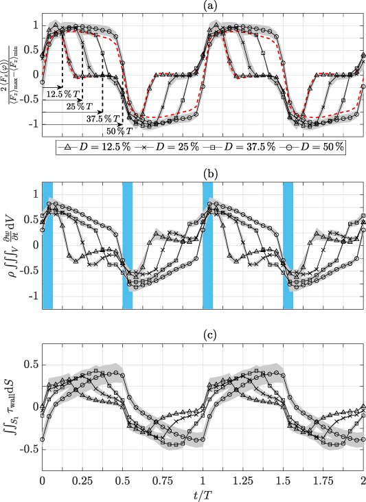
Figure 10. Estimated body forces (a) and selected terms (b), (c) according to equation (5) for  (f = 50 Hz) for case BM. (a)
  ; periods of discharge are indicated. Red dashed lines indicate the sum of (b) and (c) for D = 12.5 and 50%. (b) Acceleration term
  . (c) Self-induced drag
  . Data normalized by
  between −1 and 1. The gray shadings show the uncertainty margin of PIV experiments at different input force Fz
. Light blue shaded areas indicate application of the reduced method [16].
between −1 and 1. The gray shadings show the uncertainty margin of PIV experiments at different input force Fz
. Light blue shaded areas indicate application of the reduced method [16].
Download figure:
Standard image High-resolution imageThe arrangement of the body forces on the time axis is such that the discharge is triggered at  , thus ensuring the discharge onset to collapse on a single position on the temporal axis for all parameter combinations of D and f. Therefore, the first phase position
  of all plotted data for case BM is accordingly related to this discharge onset.
All curves for  collapse to one branch for
  . The drop of the force magnitude to
  saliently depends on D, marking the end of the discharge period. A separate analysis of individual terms in equation (5) is carried out by showing the temporal acceleration and the self-induced drag from wall-shear stresses in figures 10(b) and (c), respectively. In order to clarify the contribution of these terms to the total body force, the normalization is identical to figure 1(a). Accordingly, the temporal acceleration represents about 70% to 80% of the body force in the beginning of the actuation period
  , as visualized by the light blue shaded area in figure 10(b). These also indicate the regions of interest applied for the reduced method [16]. Over time the temporal acceleration decreases as the wall jet develops and approaches, yet never arrives to, quasi-steady conditions. The wall-shear stress in figure 10(c) undergoes the inverse behavior, growing along the discharge period and accounting for about 40% to the force for
  at the end of a half period. As a result, the red dashed lines in figure 10(a) for D = 12.5 and 50% depict that the estimated body forces are mainly a combination of temporal acceleration and wall-shear stress.
As an intermediate summary, the duty cycle can be approximately deduced from the identified body-force characteristics, furthermore, showing that the burst-modulation mode operation leads to a constant input amplitude of body force. This important finding verifies the applicability of the momentum balance according to equation (5) to highly unsteady discharge phenomena, such as body-force oscillations. Even though, for the reduced method the problem that the flow field is not at rest at  persists, based on the results in figure 10, it is recommended to apply the reduced method in combination to the integral approaches, in order to gain spatial body-force information. This requires to acquire the very first velocity fields in the beginning of the first oscillation cycle after actuation. As the needed velocity information was not available (see description of data acquisition in section 3.1) the reduced method could not be applied and remains to be an effort for future investigations. Not knowing the pressure field, the reduced method can become a valuable evaluation tool for such unsteady actuation concepts.
5.4. Body-force characteristics: oscillation frequency
The temporal progression of the body-force magnitudes for different oscillation frequencies f is shown in figure 11 for case BM. In figure 11(a) the forces of each PIV experiment were normalized and all curves for the same f were averaged, while uncertainty margins (gray shadings) were included. Note that the abscissa scaling—in contrast to figure 10—is in real time units as f is variable. The organization of the body forces in figure 11 is synchronous to figure 6(b).
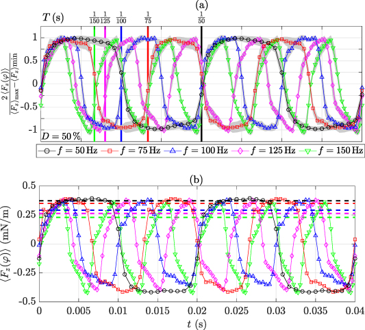
Figure 11. Estimated body forces for  Hz for case BM, D = 50%. (a) Normalized distribution of
  . (b) Absolute distribution of
  at constant time-averaged actuator power
  W. Data in (a) normalized between −1 and 1. The gray shadings in (a) indicate uncertainty margins of all curves of constant f. Dashed lines in (b) represent
  .
.
Download figure:
Standard image High-resolution imageThe rising branches at t = 0 (discharge onset) all collapse to a single curve independent of f. Since the phase resolution of the oscillation cycle was identical for all experiments, the amount of data points is concentrated and expanded in time as f increases or decreases, respectively. After a duration of t = 0.02 s the branches of f = 50, 100 and 150 Hz re-collapse, while the number of produced oscillation cycles is different by the ratio of oscillation frequencies. Accordingly, after one oscillation cycle with f = 50 Hz, the curves for f = 75 and 125 Hz have not re-collapsed, as the PA generated a non-integer number of oscillation cycles during that time. All curves coincide again at t = 0.04 s, where for the frequency range (ascending order) 2 to 6 oscillation cycles were produced. This clarifies that the body forces emerge identically independent of f after discharge onset.
In figure 11(b) absolute body-force magnitudes are compared at constant P for f = 50 to 150 Hz. The rising branches of all curves at t = 0 show the same progression as on the normalized scale in figure 11(a). This is an important feature related to resonance effects that have shown to disrupt the control authority of mechanically oscillating walls [10, 12] and, therefore, limiting the control to a small Reynolds number range. The role of resonances for PA-based oscillations can be ruled out, as a constant power input results in the same absolute body-force magnitudes independent of f.
Another relevant peculiarity is depicted by the dashed lines in figure 11(b), each of which represents the time-average of the respective body-force magnitude  . Hereby, the time-average was performed for the respective burst-duration time, equivalent to a half period of the oscillation cycle as for the entire period the force would yield zero per definition. The plateau of about constant force, as mentioned in section 5.3, is most significant for f = 50 Hz. Accordingly, the time-mean (black dashed line) agrees well with the maximum body force. Both values in the experiment have to be identical, as explained in section 5.3. An increase of f, however, produces a systematic error of the forces time-mean that culminates in about 40% when compared to the value for f = 50 Hz. This is because the majority of data points remains on the rising force branch for larger f. The coincidence of both these curves and the absolute force magnitudes and the fact that applying a constant
  , in the experiment, immediately triggers a constant body force, however, clarifies that the
  must be identical independent of f. In consequence, a sufficiently long oscillation period has to be considered, in order to receive an accurate estimation of the time-mean of forces. Henceforth, the forces will be extracted from the f = 50 Hz experiments for case BM and applied to f = 75 to 150 Hz.
The body forces of case BF in figure 12 reveal a completely different behavior when compared to case BM. The most prominent difference is due to the fact that  is a function of time. Therefore, the force is not piecewise constant across one burst duration anymore but also time-dependent [34]. This characteristic is well-described by the force curves in figure 12(a).

Figure 12. Estimated body forces for  Hz for case BF. (a) Normalized distribution of
  . (b) Absolute distribution of
  at constant time-averaged actuator power P = 1.9 W. Data in (a) normalized between −1 and 1. The gray shadings in (a) indicate uncertainty margins of all curves of constant f. Lines in (b) represent
  .
.
Download figure:
Standard image High-resolution imageThe style of figure 12 is somewhat different from figure 11 for the following reasons. The  envelopes are sine waves (see figure 1(b)), where the maximum body force is generated for
  . The discharge onset in this case is dictated by the breakdown voltage for the given dielectric barrier and fluid [34]. Therefore, changing the amplitude of the
  envelopes leads to a widening or narrowing of the discharge period and the point in time inherent to the discharge onset is earlier or later, respectively. This attribute renders the discharge onset the wrong quantity for comparing the body forces across the parameter combinations. A more suitable means to organize the body forces on the time axis is to assign
  to the position
  . This is because the duty cycle develops symmetrically around
  , which corresponds to
  . This has been done in figure 12, where all body-force distributions start at t = 0,
  . It is further to be noted here that the alignment style of body-force magnitudes in figure 12 is also different from the respective fluid response in figure 6(c), for the above-described reasons. As such, the position of the strongest force magnitude is indicated in figure 6(c) as to support synchronization of the presented body-force and fluid-response curves.
Both in figures 12(a) and (b) the body force curves, starting at t = 0, follow their own slope which becomes steeper with increasing f. This is very conclusive, since for larger f the slope of  , being coupled to
  , is steeper. As the voltage and force do not scale linearly [16, 17], the sinusoidal shape of
  is not present in figure 12. The peak-to-peak magnitudes of the absolute body forces in figure 12(b) agree well, except for the rising branch for f = 75 Hz that culminates in a too large magnitude. The curves were also checked for the time-mean values, other than for case BM, clearly showing a non-systematic deviation of ±8% (Note the compression of the ordinate in figure 12 as compared to figure 11). Therefore, for case BF an estimation of the body forces can be done independent of f. A last noticeable feature is the shift of
  with respect to
  . This shift was already indicated in figure 6(c). The reason is that the flow is further accelerated past
  (or
(or  ) until
  undercuts the breakdown field strength.
5.5. Parametric effects and performance analysis
The remaining part of this investigation concerns the independent parameter effects for both excitation modes on the PA performance of a near-wall oscillator. Recalling the electrode arrangement (see figure 1), the wavelength λz
of the discharge is one crucial geometrical parameter as the fluid ideally travels from one edge to the opposite one within half oscillation period. Analogously, an oscillating wall would undergo one peak-to-peak stroke during that time [10, 12]. For the PA λz
is comparable to the stroke length and, therefore, one can define a characteristic velocity of  that gives a measure of the covered z distance by the oscillation. A second meaningful measure for the PA performance is the relation of input amplitude and output flow. The first quantity is described by the integrated effect of the body force
  estimated for the selected control volume. The extension length of the force in the horizontal direction ideally converges to the width of the encapsulated electrode with increasing body force. The total induced energy can be defined as the specific energy of the flow
  imposed along the z direction. The relation of these relevant quantities, closely resembles a classical Pareto front and is shown in figure 13, where the abscissa indicates the energy ratio and the ordinate refers to the amplitude of the virtual wall velocity normalized with
  . In the numerator of the abscissa values, the spanwise wavelength λz
is applied instead of the force penetration length [17], as the spatial body-force distribution was not accessible. This, as a result, will not change the shape of the curve but the data is compressed on the abscissa here.
. In the numerator of the abscissa values, the spanwise wavelength λz
is applied instead of the force penetration length [17], as the spatial body-force distribution was not accessible. This, as a result, will not change the shape of the curve but the data is compressed on the abscissa here.

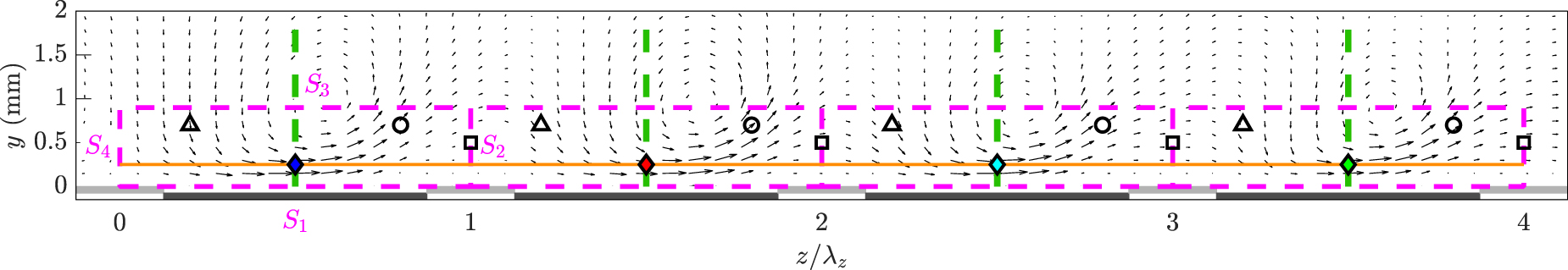
Figure 13. Performance diagram for cases BM and BF. (a) Maxima of  and
and  . (b) Time-mean of
  and
and  for a half oscillation period. Parameter-related symbols can be retrieved from figures 2 and 3.
Download figure:
Standard image High-resolution image
It is found that the data collapse to a single curve independent of the excitation mode (case BM or BF). In figure 13(a) the maximum values over one oscillation period are considered, as similarly done for an oscillating wall [12]. In this case the maximum amplitude is large enough to exceed  . Moreover, the more rigorous time-mean over one oscillation period as elaborated in section 4.2 is shown in figure 13(b). Accordingly, the amplitude decreases and reaches a value of about 0.85. As the data for either maximum or time-mean values both lie all on a single curve, the parametric effects are conserved in both graphs. Therefore, a single snapshot of the same phase position in the oscillation cycle suffices the extraction of the behavior of plasma-induced flow oscillations. Both graphs clarify that for large f and small D the body force, if being increased, can be more efficiently transformed into fluid momentum. For lower f this effect is much weaker, as observed by the larger slope. On the other hand, for low f and large D an amplitude of one appears more accessible. This is, however, only partially representative of the system performance, since the influences of both changing geometrical parameters and external flow were not considered in the present study.
The influencing effects of all parameters (input amplitude Fz
, duty cycle D, oscillation frequency f and wavelength λz
) are sketched in figure 13(b) by the inserted arrows. Accordingly, an increase of the distance between two discharges (λz
) demands for an increase of Fz
or D. The same holds true for larger f. The increase of Fz
or D can be compensated by increasing either f or λz
. Both increase of  and decrease of λz
involve a quadratic effect on
and decrease of λz
involve a quadratic effect on  (see abscissa in figure 13(b)), therefore increasing the performance. The spanwise wavelength λz
is, however, not an independent parameter, because the combination of the width of the exposed and encapsulated electrodes (equal to λz
), have a significant effect on Fz
. As such, an increase of λz
, by increasing the width of the exposed electrode hampers the increase of
(see abscissa in figure 13(b)), therefore increasing the performance. The spanwise wavelength λz
is, however, not an independent parameter, because the combination of the width of the exposed and encapsulated electrodes (equal to λz
), have a significant effect on Fz
. As such, an increase of λz
, by increasing the width of the exposed electrode hampers the increase of  because the available length of the electric field above the encapsulated electrode remains constant. Hence, the width of the exposed electrode is recommended to be chosen as narrow as possible.
For case BF the duty cycle D, being a function of the input amplitude Fz
, is another relevant dependent parameter. The limiting factor is a too large input voltage, producing opposing discharges as D increases accordingly. This is because the breakdown field strength of air and the dielectric relative permittivity remain constant, whereas the excess area of the breakdown barrier increases by increasing the input voltage, which is equivalent to an increase of Fz
. In order to further improve the performance, either the dielectric material can be replaced (changing the dielectric relative permittivity or the dielectric layer thickness) or one could operate the actuator at higher plasma frequencies  . Since the force is shown to increase with increasing frequency
  at constant operating voltage V, an increased frequency at constant force in turn is maintained for the desired lower operating voltage.
6. Conclusions
In the current work, plasma-induced flow oscillations serving as surrogates to spanwise wall oscillations for turbulent flow control were triggered using the burst-modulation [32, 33] and beat-frequency [31, 34] modes. The discharges were generated on an electrode array that features the exposed electrode to be the mandatory minimum discharge discontinuity [33, 34]. The comparisons of plasma-induced flow oscillations both mutually and to the oscillating wall analogue (i.e. Stokes layer) were carried out on the grounds of time-dependent body-force magnitudes (equation (5)) and virtual wall velocities (equation (8)).
The produced integral body force was found to be a combination of the reduced method by Kotsonis et al [16] and Versailles et al [29] and is mainly the result of temporal acceleration and wall-shear stress or PA self-induced drag. In the present study, the acceleration term was found to account for up to 80% of the total force in the beginning of each oscillation cycle. For the burst-modulation mode (case BM) the body-force magnitude logically forms a plateau of about constant force. Because the peak-to-peak voltage is time-variant for the beat-frequency mode (case BF), the force magnitude changes continuously. The characterization in quiescent air is a requirement that aids the fluid-mechanic understanding of the implications of the PA and, typically, the evaluation of force magnitudes is sufficient. However, the body-force distribution is a vital tool to feed numerical simulations and can be exploited to minimize the efforts of investigating a wide spectrum of parameters in experiments. Accordingly, the outcomes of the force characteristics (see sections 5.3 and 5.4) reveal two recommended options to gain the spatial force distribution:
- to capture the period from resting fluid to the actuation of the plasma-induced flow oscillation at a high sampling rate and applying the reduced method [16]
- to acquire the PA-induced velocity field in quasi-steady conditions for the identical PA and operating conditions, in order to apply the common differential methods [17, 18, 46]
This procedure is straightforward for case BM, as  , but requires a sequence of measurements for case BF, where
  is a function of time. Finally, it is concluded that the outcomes and the derived approaches allow for enhanced numerical simulations of plasma-based oscillations, where promising parameter combinations can be retroactively investigated in experiments.
From the comparison of the absolute body-force magnitudes of cases BM and BF, frequency-dependent resonance effects were ruled out. Typically, mechanically oscillating walls work well at the resonance frequency which constricts their application to a narrow Reynolds-number band. Based on the findings for plasma-induced flow oscillations, the input force remains constant independent from f, indicating that PAs can cover a broader range of Reynolds numbers than oscillating walls.
The fluid response of the investigated oscillation concepts is distinctively different, yielding a discontinuous waveform (due to the burst actuation) for case BM and a sinusoidal (Stokes-layer-like) waveform for case BF (see figure 6). This is particularly important as the waveform type has an impact on both control effect and efficiency [15]. However, for case BM the ability to manipulate the waveform by changing the duty cycle has revealed another advantage over the beat-frequency mode. The decrease of the duty cycle leads to less-pronounced vertical velocity components and reduces the self-induced drag (see figures 9 and 10). The conclusion from these outcomes for the application in a boundary-layer flow is to select rather short duty cycles, in order to avoid both adverse vertical motions and additional self-induced drag upon the streamwise flow-induced friction drag.
The performance analysis of the plasma-based oscillation led to a universal diagram valid for cases BM and BF that wraps up the effects of operational and geometrical parameter combinations on the induced momentum caused by the supplied body force. It renders the choice of parameter combinations and excitation modes irrelevant as the transfer function is identical, based on integral values of the momentum transfer. Therefore, snapshots of a single phase-locked position in the oscillation cycle satisfy the performance evaluation, reducing the experimental characterization efforts. Independent of the excitation mode one can move back and forth on a single curve by changing individual PA parameters.
As a final remark, all PA parameters have to be chosen carefully under ultimate consideration of the inherent characteristics of the underlying flow, as also analysed on a conceptual basis by Hehner et al [33] for a fully-developed turbulent channel flow scenario [12]. Correspondingly for the current work, the success of flow control, as also emphasized in section 5.5, depends on the ability—beyond the presented results—of choosing suitable parameter combinations, matching both actuation parameter space and spatio-temporal flow characteristics. Uncovering cause-effect relations and mutual interrelationships of plasma-induced flow oscillations and turbulent flow will, therefore, be foreseen for near-future investigations.
Acknowledgment
The authors acknowledge technical support with the Minipuls devices from SLA at TU Darmstadt.
Data availability statement
All data that support the findings of this study are included within the article (and any supplementary files).