

Abstract
Investigation of excitation spectra of liquids is one of the hot test topics nowadays. In particular, recent experimental works showed that liquid metals can demonstrate transverse excitations and positive sound dispersion. However, the theoretical description of these experimental observations is still missing. Here we report a molecular dynamics study of excitation spectra of liquid iron. We compare the results with available experimental data to justify the method. After that we perform calculations for high temperatures to find the location of the Frenkel line introduced in our previous works.
Export citation and abstract BibTeX RIS
Introduction
In solid state physics one of the main characteristics of a crystal is its excitation spectrum (phonons, magnons, etc). The study of collective excitations in liquids started much later. However, nowadays it is clear that excitation spectra of liquids are of great importance for understanding their properties. In particular, two phenomena are now of great interest: positive sound dispersion and transverse excitations in liquids.
Until now, it has often been claimed that a liquid cannot sustain transverse excitations. Many basic textbooks even state this as the main difference between liquids and solids. However, it is already known for a long time that viscous fluids do sustain shear waves. As early as in 1973 it was shown in a seminal set of works on simulation of a Lennard-Jones (LJ) fluid, it was shown that a LJ system can support transverse excitations [1]. So, it was predicted that liquids with a low viscosity also can demonstrate transverse excitations.
It took much more time to find transverse excitations in low viscosity liquids experimentally [2–7]. They were observed in several metallic melts, including molten iron, copper, gallium, etc. One can expect that other liquids should also demonstrate transverse excitations and further experimental study is required.
Transverse excitations can be related with another phenomena—positive sound dispersion (PSD), which means that the speed of excitation at some wave-vector  exceeds the adiabatic speed of sound cs. Positive sound dispersion was experimentally observed in a number of different liquids including liquid metals [2–8], water [14], nitrogen [15], germanium oxide [16] and other liquids. Moreover, numerous simulations confirmed the presence of PSD in different systems, for example, in liquid lithium [17], gallium [18] and some other liquids. In our recent works [12, 13] a simple phenomenological analysis of the origin of PSD was performed. Moreover, it was shown in [13] that transverse excitations of LJ fluid fluid exist below the Frenkel line and do not exist above it. However, the understanding of this phenomenon is still incomplete.
Although transverse excitations were found in liquids, they cannot be observed in gases. It is of special interest since a liquid can be transformed to a gas without any phase transition. It means that following some phase transition-free path, one should observe some kind of disappearance of transverse excitations. In our recent works we proposed a line called the Frenkel line separating regions of different microscopic dynamics [9–12]. Below the Frenkel line the fluid is liquid-like, while above the line it is gas-like. Several definitions of the Frenkel line were proposed. However, the most general definition from our point of view is that the Frenkel line is the line where transverse excitations in the fluid disappear [13]. It leads to some important consequences. For example, the isochoric heat capacity of a monatomic fluid at the Frenkel line is equal to 2kB per particle.
Another important feature of the Frenkel line is that velocity autocorrelation functions (VACFs) lose the oscillating behavior at this line. The heat capacity ( for a monatomic fluid) and VACFs criteria can be used as simple methods for finding the location of the Frenkel line on the phase diagram. The Frenkel line of several model and real fluids was recently calculated using these criteria [9–11, 19–24]. In particular, the Frenkel line of liquid iron was reported in [24]. The Frenkel line was experimentally studied in [25].
The present work extends our previous investigation of the Frenkel line to real systems. We calculate the dispersion curves of liquid iron under experimental conditions [2] and show that the results of simulations are in agreement with the experimental ones. Using these results, we extend our calculations to higher temperatures in order to find the location of the Frenkel line and its relation to the dispersion curves, heat capacities and VACFs.
System and methods
In the present study, we simulated a system of 3456 iron atoms by molecular dynamics methods. The particles were placed in a cubic box with periodic boundary conditions. Their interaction was simulated by the EAM model proposed by Belonoshko et al [26]. The density of the system was fixed to  and the temperatures varied from
  K up to
  K. The EAM potentials are developed for simulation solid and liquid metals. This model is not applicable to gas phase of metallic systems. However, all pressure-temperature points studied in the present paper belong to condensed phase which can be seen from the values of pressure. Therefore, EAM model should be at least qualitatively correct in these points. The system was first equilibrated at a given temperature in the canonical ensemble and was then simulated in the microcanonical ensemble for computing averages. The timestep during the equilibration run was set to
  fs and the run itself consisted of
  steps. The production run was
  steps with a step of
  fs. Such a small step was necessary in order to resolve the small time behavior of time correlation functions with high precision. Useful recommendations on the selection of the simulation parameters can be found in [27].
From our simulations we computed the VACFs and the excitation spectra of liquid iron. The spectra were determined in the following way. From our simulations we calculated the longitudinal and transverse parts of velocity flux correlations:

and
where  is the velocity current and the wave vector
  is directed along the z axis [28, 29]. Dispersion curves of longitudinal and transverse excitations can be obtained from the location of maxima of Fourier transforms
  and
and  respectively.
In order to find whether PSD occurs at a certain temperature, one also needs to know the adiabatic speed of sound cs. The speed of sound was obtained from the well-known relation  , where
  . The isochoric heat capacity is obtained from kinetic energy fluctuations in the microcanonical ensemble:
  [30]. For the isobaric heat capacities, extra simulations were performed along isobars corresponding to the pressures at studied points, but at higher and lower temperatures and the heat capacity was computed by numerical differentiation of the enthalpy:
  .
.
Results and discussion
As was mentioned above, the dispersion curve of liquid iron was measured experimentally in [2] where excitation spectra of liquid iron at a temperature of 1823 K were given. We begin our study with a comparison of our simulation results with the experimental data from [2] in order to justify the simulations. For doing this, we performed simulations at the very close temperature of 1850 K. The excitation frequencies are given by the location of the peaks of Fourier transforms of the velocity flux correlation functions. Figure 1 shows examples of spectra of transverse part of the velocity current correlation function. One can see that while at the lowest wave vector the only peak corresponds to zero frequency, at the larger k-vectors peaks at finite frequencies appear. The results are given in figure 2. One can see that molecular dynamics results are in good agreement with experimental data for the case of longitudinal excitations. Small deviations close to the pseudo-Brillouin zone boundary can be attributed to uncertainties of both the simulation and experiment. Although molecular dynamics simulations give a slightly higher speed of sound ( from simulation versus
  from experiment), the overall agreement is remarkably good. Importantly, strong PSD is observed both in experiment and simulation.
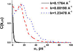
Figure 1. Fourier transform of transverse part of the velocity flux correlation function at  K and three k-vectors.
Download figure:
Standard image High-resolution image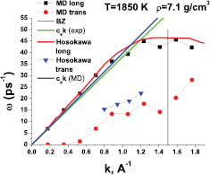
Figure 2. Comparison of excitation spectra of liquid iron obtained in this work with experimental results from [2].
Download figure:
Standard image High-resolution imageThe experimental frequencies of transverse excitations are slightly higher than these from simulation. This difference can be due either to the EAM model, which was developed to simulate the melting line of iron at high pressures rather than the dynamical properties, or to experimental errors.
In our previous work, we calculated the location of the Frenkel line of iron [24]. Here, we repeat the calculations of the Frenkel temperature of iron by both the heat capacity and VACF criteria at a density of  . Figure 3(a) reports the VACFs of liquid iron at the given density and several temperatures. One can see that VACFs demonstrate an oscillating behavior at low temperatures, whereas the oscillations disappear at higher temperatures. From this plot, the Frenkel temperature is estimated as
  K. The same temperature is obtained from the heat capacity criterion (see figure 3(b)). The pressure at TF is
  GPa.
GPa.
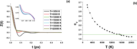
Figure 3. (a) Velocity autocorrelation functions of liquid iron at the isochor  ; (b) isochoric heat capacity at the same isochor.
Download figure:
Standard image High-resolution imageIt was recently demonstrated in [13] that the qualitative changes of excitation spectra of Lennard–Jones (LJ) fluid are attributed to the Frenkel line [13]. However, the calculations of dispersion curves in simulation always involve large computational errors, which complicates the situation and prevents using the disappearance of PSD and transverse excitations for precise location of the Frenkel line. Here, we extend these investigations for liquid iron. From figure 2, one can see that strong PSD occurs in the system. Figure 4 show the excitation spectra at three different temperatures: below the Frenkel line, at the Frenkel line and above it. The speeds of sound at these temperatures are  at
at  K and
K and  at
at  K. The pressure at
  K is 7.56 GPa.

Figure 4. Spectra of liquid iron at three temperatures: below the FL, at the FL and above it.
Download figure:
Standard image High-resolution imageBoth PSD and transverse excitations are observed below the Frenkel line (see figure 4). At  K, which corresponds to the FL both phenomena disappear and above the Frenkel line, neither PSD nor transverse excitations occur in the system above the Frenkel line. This scenario is in perfect agreement with the case of the LJ fluid discussed in our previous work [13].
In order to validate the results we have performed additional simulations of excitation spectra of liquid iron at higher density  . The results are given in figure 5. One can see that the behavior of the excitation spectra at this density is qualitatively similar: transverse excitations and positive sound dispersion are observed at low temperature, but not at the high one.

Figure 5. Spectra of liquid iron at density  and two temperatures: below and above the Frenkel line.
Download figure:
Standard image High-resolution image
In general, liquid metals can be considered as relatively simple liquids. Near the melting line, they differ from the noble gases by many-body interactions because of the electron gas contribution. However, the contribution of many-body interactions at high temperatures or high pressures becomes small compared to the pair interaction. As a result, the liquid metals can be effectively approximated by simple systems with pair interactions, which were actively used to construct perturbation theory for liquid metals (see, e.g. review [31] and references therein). In [32], the properties of liquid iron along the melting line were projected onto the behavior of the same properties of the soft sphere system, i.e. the system with inverse power-law interaction between the particles. The results of this work also confirm that liquid metals at high temperatures behave very similar qualitatively to noble gases.
In conclusion, we have performed a molecular dynamics simulation of liquid iron. We have found the Frenkel temperature at  and have calculated the dispersion curves close to the melting line and at three different temperatures above the melting line. The results at a low temperature are in good agreement with experimental data. The qualitative behavior of the spectra of both longitudinal and transverse excitations confirm the interpretation of the Frenkel line as a line of qualitative change in the excitation spectra.
Acknowledgments
We are grateful to the Russian Scientific Center at the National Research Center Kurchatov Institute and to the Joint Supercomputing Center of the Russian Academy of Sciences for access to computational facilities. This work was supported by the Russian Science Foundation (Grant No 14-22-00093).