

Abstract
The accurate characterisation of a copper–beryllium wire with a diameter of 0.1 mm is one of the steps to increase the precision of future accelerators' pre-alignment. Novelties in measuring the wire properties were found in order to overcome the difficulties brought by its small size. This paper focuses on an implementation of a chromatic-confocal sensor leading to a sub-micrometric uncertainty on the form measurements. Hence, this text reveals a high-accuracy metrology technique applicable to objects with small diameters: it details the methodology, describes a validation by comparison with a reference and specifies the uncertainty budget of this technique.
Export citation and abstract BibTeX RIS

Original content from this work may be used under the terms of the Creative Commons Attribution 3.0 licence. Any further distribution of this work must maintain attribution to the author(s) and the title of the work, journal citation and DOI.
1. Introduction
The European Organisation for Nuclear Research (CERN) is designing a 48-km long compact linear positron–electron collider called CLIC. CLIC would accelerate particles in opposite directions and focus them within an elliptical beam of 1 nm × 40 nm, reaching an energy of at least 3 TeV at the collision point. Critically, CLIC performance relies on the pre-alignment of several thousands of magnets and accelerating structures of which the magnetic axes have to lay within 200 m long cylinders with diameters of 14 µm or 17 µm [1]. However, in 2012 the pre-alignment methods of the accelerator's components could not guarantee better than 20 µm diametral positioning errors [2]. To address CLIC's pre-alignment objectives, the PACMAN project (Particle Accelerator Component's Metrology and Alignment to the Nanometre scale) has been funded [3] to develop alignment procedures based on fiducials, which are alignment targets located on the components [4]. Before final assembly, the fiducials are measured in a metrology laboratory and then elements of the accelerator are pre-aligned on 2-m long girders using a stretched wire, which is nominally superimposed on each component axis [5]. The fiducials and the wire are measured using a coordinate measurement machine (CMM) from which the final relative position of each component for the final assembly of the accelerator is inferred. The tolerated error on the wire axis coordinate measurement is in the order of hundreds of nanometres. Such low measurement errors demand well-known dimensional characteristics of the pre-alignment wire [6].
In PACMAN, a 100 µm diameter copper and beryllium (Cu 98%; Be 2%) wire is used. The wire is designed to withstand a tension higher than 1 kg and has a linear mass lower than 70 mg m−1. The diameter of the wire varies less than 5 µm and its behaviour is unaffected by magnetic fields. Details of the measurement of these characteristics are presented elsewhere [7]. Concomitantly, the wire's form error has to be less than 0.5 µm which entails a measurement system able to measure form errors with an uncertainty smaller than 0.1 µm at a confidence level of 95% [8]. This paper completes the wire's quality evaluation by summarising form error measurement results.
Current commercial instruments are not designed to measure micrometre form errors of small diameter long wires with tens of nanometres uncertainty. The measuring capability of the commercial systems is limited by: the fast increasing slopes of the wire surface, which restricts the instrument to probe accurately the cross-section of such samples; the environment that easily disturbs the stretched long sample; and the lack of freedom to move around the sample. A measurement system that overcomes these problems is described in this article.
After this short introduction, the second section focuses on the form measurement strategy, the third section details the uncertainty evaluation while the fourth section gives the results of the measurements. This paper is completed by the discussion in the fifth section and the conclusion in the sixth section.
2. Form measurement setup
The setup used to measure the form errors of the wire is depicted in figure 1. The wire is mounted on a high precision rotary table while the non-contact sensor is rigidly fixed to the base. The base of the rotary table MarForm is isolated from the ground vibrations using passive damping. While the wire spins around its axis at a constant velocity, the optical sensor records the relative surface displacement. The form error is the sum of the extremal deviations to a circle built using the Gauss approximation.
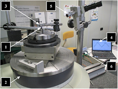
Figure 1. The sample (1) is held by the chuck on the rotary table (2), while the chromatic confocal sensor (3) is observing its surface. On the computer screen (4), the acquisition can be seen. Behind the holder of the magnifying lens used for pre-alignment (5), the controller (6) displays the distance in real time.
Download figure:
Standard image High-resolution imageThe sensor used for this application [10] is a point chromatic confocal sensor produced by Precitec, having 100 µm measurement range and using a white light beam focused in a 3.5 µm large spot, and analysed by a CHRocodile S. The principle of the chromatic confocal sensor is the following (see figure 2): the light coming from a polychromatic source illuminates the sample's surface after being focused by a microlens which introduces a strong axial chromaticity. The light reflected by the sample is focused on a surface with a pinhole before it reaches the sensor. This pinhole acts as a filter removing the light rays unfocused in its plane, which reduces the spectral range of the light waves reaching the sensor. These waves' spectrum is analysed: a peak in intensity appears at the wavelength which was in focus on the sample's surface. This wavelength is linked to the distance separating the sample's surface and the sensor's reference optical plane after calibration.
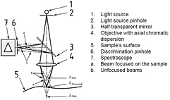
Figure 2. Schematic of the principle of the chromatic confocal sensor Reproduced with permission from [9]. The extracts from the standard ISO 25178-602:2010 – Geometrical Product Specifications (GPS) — Surface Texture: Areal — Part 602: Nominal Characteristics of Non-Contact (Confocal Chromatic Probe) Instruments are reproduced courtesy of AFNOR. Only the original and complete text of the standard as it is provided by AFNOR Editions – accessible via the internet website www.boutique.afnor.org – has a normative value.
Download figure:
Standard image High-resolution image3. Uncertainty evaluation of the wire form measurement
Given the setup presented in section two, the main sources of uncertainty affecting the form measurement have been grouped into three main categories:
- the confocal chromatic sensor's measurement uncertainty;
- the post-processing effects and the environmental conditions;
- the misalignment errors and the rotary table imperfections.
Each of the above uncertainty contributions is detailed in the following paragraphs. Their effect will be summarised in the form of distributions and associated standard deviations. The uncertainty evaluation was based on the Guide to the Expression of Uncertainty in Measurement [11] applied with help from the Measurement Uncertainty Analysis Principle and methods [12]: a handbook written by the National Aeronautics and Space Administration.
3.1. Chromatic confocal sensor—traceability evaluation
Manufacturer specifications include the following nominal characteristics of the sensor: axial resolution of 4 nm, repeatability of 10 nm and accuracy of 30 nm. However, these characteristics do not account for the effects of sample intrinsic properties, such as surface roughness, reflectivity and colour, which will influence the measurement output of the sensor [13].
To evaluate the uncertainty contribution of the sensor traceability and scale linearity combined with the effects of the wire intrinsic properties, a comparison between a contact probe and the chromatic confocal sensor has been performed.
The device used as a reference in this measurement is the MarForm evaluating device, traceable to the national standards with 50 nm of uncertainty after 50 rpm low-pass filtering. The sample used for the comparison measurement is a 5 mm diameter steel gage. The contact probe used for the comparison has a diameter of 3 mm. The two measurements used for the comparison have been performed simultaneously in a temperature-controlled room, by the two sensors mounted on the same base passively damped. The mounting was similar to the one shown for the 1 mm large gage on figure 3. The measurement lines were as close as possible to each other: the alignment was made with an optical magnifier comparable to the one shown in figure 9, in the field of which both the light spot and the contact point of the probe-tip were visible.
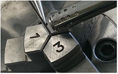
Figure 3. Chromatic confocal sensor versus contact measurement on a 1 mm diameter cylinder gage (top-down view).
Download figure:
Standard image High-resolution imageThe radius of the contact probe has a filtering effect: all the peaks are taken into account whereas some valleys are not, since the contact probe cannot reach their bottoms. The optical non-contact probe has a much smaller filtering effect due to the shape of its light cone and its 3.5 µm large spot size [14]. To reduce the outliers' impact, a low pass Gaussian filter with a cutting wavelength of 3.5 µm is applied to the raw dataset. In order to compare the form error deduced from the measurement, the data acquired without contact are filtered. Only the position of the point the closest to the surface for a given point is kept by the algorithm, as this point corresponds to the extremal position reached by the probe tip (see figure 4). This filter is applied to the form measurement dataset with the curvature of the sample neglected.
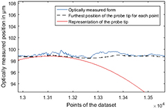
Figure 4. Chromatic confocal sensor's form measurement on a 5 mm in diameter cylinder gage with representations of the contact probe-tip approaching the surface and the limit reached by the probe-tip.
Download figure:
Standard image High-resolution imageThe results of the comparison show a difference of a few hundred of microns. This is due to the gage used for the measurement—see section 5 for more details. Using this setup and the filters described above, the system was traceable with 300 nm standard uncertainty.
3.2. Post-processing and environment
The form errors are calculated using the raw distance measurements in two steps. First, the sinewave due to the sample's decentring, which can be observed in figure 5, is removed from the data. Then, in the second step, the form error is calculated from the extremal positions of the data, as shown in figure 6.
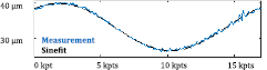
Figure 5. Distance profile, obtained with a chromatic confocal sensor, with the fitted sine curve as a function of the scanned position (kilo data points).
Download figure:
Standard image High-resolution image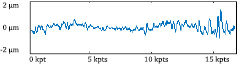
Figure 6. Form measurement as a function of the position (kilo data points): average of seven measurements, obtained with a chromatic confocal sensor, after removal of sinusoidal fit.
Download figure:
Standard image High-resolution imageAn estimation of the environment effect on several measurements showed that it is reduced to a few tens of nanometres by controlling the room temperature and isolating the rotary table from the ground as explained in section 2.
The noise of the repeatability measurement is the residual after the extraction of the mean, which contains the information on the form (see figure 7). It is composed of the confocal chromatic sensor's measurement noise, the rotary table imperfections, the environment noise and the uncertainty of the post-processing. The probability distribution of this noise was assumed to follow a normal distribution. As a result, its uncertainty can be expressed with its standard deviation as follows in equation (1):

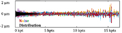
Figure 7. Residual noise after removal of mean profile and its distribution as functions of the position and the number of data points (kilo data points) for seven measurements.
Download figure:
Standard image High-resolution imageA Monte-Carlo simulation based on the post-processing algorithm revealed the uncertainty on the form error evaluation as a function of the amplitude of a white noise applied to a form measurement extracted as described above. When using the output of this simulation as uncertainty contribution, several assumptions are done. Firstly, the noise from the environment is considered white and with a constant standard deviation during the measurement period whereas it consists in the temperature deviation and high-frequency oscillations. In other terms, the temperature is considered constant. Secondly, the input of the Monte-Carlo simulation is the mean of a repeatability measurement. Thus, considering the output as the uncertainty for a series of measurements, one considers the form composition of the samples of this series to not differ much from the form composition of a typical sample of this series on which was done the repeatability measurement input of the Monte Carlo simulation.

3.3. System setup
The influence due to the sensor's misalignment includes the following components:
- Angle α between the sensor and the sample's surface normal. The manufacturer provided the maximum possible error induced by the angle α for the sensor (see table 1), which includes the fact that the sensor's spot on the surface is distorted. The angle α can be divided into two components, αθ and αz, as follows:
- αz is the vertical angle as depicted in figure 8. It can be easily reduced below 5° using the eye and a magnifying glass (see figure 9). It increases the sensor uncertainty following the table 1, and αz = 5° induces a negligible cosine error of 12 nm according to the equation (3):

- αθ is the horizontal angle as depicted in figure 8, which increases with the distance between the optical axis of the sensor and the wire centre (influenced by the quality of the cresting and the sample decentring), following the sine equation (4):
- αz is the vertical angle as depicted in figure 8. It can be easily reduced below 5° using the eye and a magnifying glass (see figure 9). It increases the sensor uncertainty following the table 1, and αz = 5° induces a negligible cosine error of 12 nm according to the equation (3):
- Angle β between the sample local axis and the table's axis of rotation as depicted in figure 8. It is taken into account in the angle αz.
- Angle γ between the sample's surface normal and the sample's theoretical axis due to the form error of the sample as depicted in figure 8. It contributes and increases locally the angle αθ. This angle γ can reach 30°, so it is a large source of uncertainty in the form measurement (see table 1). Nevertheless, it has a negligible impact on the form error evaluation as the extremal positions of the surface are linked to minimal angles γ.
- Distance d between the sample's axis and the table's axis of rotation: the decentring. This distance engenders a sinewave which is removed during the post-processing (see figure 5, in dashed black).


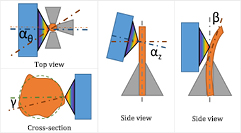
Figure 8. The misalignment angles: in orange the wire, in dark orange its actual axis or normal, in green its nominal shape, in grey the chuck, in blue and rainbow the sensor tip, in dark blue the sensor's axis.
Download figure:
Standard image High-resolution image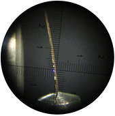
Figure 9. Chromatic confocal sensor's purple spot on a 0.1 mm in diameter wire with a misalignment angle approaching αz = 7°.
Download figure:
Standard image High-resolution imageTable 1. Variation of the misalignment angle due to the distance from the sensor's optical axis to the sample's axis for a 100 µm diameter sample, and expression of the maximum error corresponding to such an angle αθ.
| Sensor's decentring /µm | Contribution to the angle αθ /° | Extremal error associated to this contribution to αθ/µm |
|---|---|---|
| 10 | +5.7 | +0.00 |
| −0.10 | ||
| 20 | +11.5 | +0.08 |
| −0.15 | ||
| 30 | +17.5 | +0.20 |
| −0.15 | ||
| 40 | +23.6 | +0.76 |
| −0.15 | ||
| 50 | +30.0 | +1.60 |
| −0.58 | ||
During the alignment phase, special care was given to minimise the above-mentioned angles, so that the decentring was considered smaller than 10 µm and the misalignment angle αz and αθ were smaller than 10°.
The vertical and radial misalignment angles contribution to the measurement uncertainty (uα) is propagated in the form of a rectangular distribution, R(−0.13 µm, 0.13 µm) that has a variance equal to (0.13 µm)2/3.
The rotary table error is expressed by the manufacturer as the combined effect of a fixed and a measurement height dependent contribution. For the measurement configuration presented in figure 1, the maximum error induced by the rotary table is estimated to be less than 40 nm.
3.4. Total uncertainty on the measurement
The total uncertainty is influenced by the different sources previously introduced, it is expressed as follows in equation (5) and the impact from each source for an average form error appears in table 2:

with
- the total uncertainty on the result
- the uncertainties from the different sources


Table 2. Uncertainty sources and contributions for an average form error of 1.76 µm.
| Source | Standard uncertainty/nm | Contribution/% |
|---|---|---|
| Traceability | 300 | 87 |
| Processing | 87 | 7 |
| Misalignment | 75 | 6 |
| Total uncertainty | 321 | 100 |
4. Results: wire measurements
The wire was measured at 10 random positions along its length. In order to optimise the light intensity by taking into account the reflection spectrum of the copper, the measurements were performed away from the sensor: in the part of the measurement range where the light is red. The measurement results were reported in table 3.
Table 3. Results from the measurements and their uncertainties.
| Measured form error/µm | Uncertainty (2σ)/µm |
|---|---|
| 1.44 | 0.103 |
| 2.75 | 0.155 |
| 2.10 | 0.128 |
| 1.56 | 0.108 |
| 1.85 | 0.118 |
| 1.82 | 0.117 |
| 1.47 | 0.104 |
| 1.74 | 0.114 |
| 1.38 | 0.101 |
| 1.48 | 0.105 |
5. Discussion
On one hand, the results obtained by applying the methodology described in the third section (coupled with the environmental conditions of the CERN laboratory and the care of the operator) showed that it is possible to measure the form error of very small samples such as the PACMAN reference wire with an uncertainty of 321 nm. On the other hand, the methodology described in this paper and the uncertainty evaluation can be adapted to many different samples and sensors.
The obvious limitation of this design is that the measured form error added to the misalignment contribution cannot be larger than the measuring range of the sensor. Nevertheless, larger form error can be measured with a non-contact sensor having a larger measuring range (which is very often linked to a larger uncertainty). Obviously, the impact of the temperature and some other assumptions would need to be adapted to each case.
Concerning the traceability measurement, it was first assumed in this study that the lapped gage is stable enough to be considered with the same form error for the contact measurement circle and the non-contact measurement circle as they are both within a cylinder a few tens of micrometres long. The results of the comparison measurements were showing discrepancies a few hundred of nanometres large. A measurement of 10 circles on the 5 mm diameter gage was performed with the contact probe of the Mahr system. The results showed that the difference between two measurements separated by 15 µm can reach 150 nm without being filtered by the software (nevertheless, filtered by the contact probe-tip). The large uncertainty linked to the measurement traceability results from the difficulty to measure the roundness of 0.1 mm in diameter gages. It contributes greatly to the measurement uncertainty.
The aim of this study was to validate the measurement concept of the Shape Evaluating Sensor: High Accuracy and Touchless, designed and implemented by the author which aims at both evaluating the form and the position of the PACMAN reference wire with a sub-micrometric accuracy within the Leitz Infinity coordinate measuring machine.
6. Conclusion
An adapted measurement method was implemented, tested and applied to evaluate the form measurement of a 0.1 mm diameter copper–beryllium wire used as a reference for high precision particle accelerator's component pre-alignment.
The first part of this paper focused on the validation of the methodology by comparison with a traceable reference and details the sub-micrometric uncertainty evaluation linked to the measurements. Its second part focused on their application on the reference wire form evaluation, leading to the results of the form error with their corresponding uncertainties. The possibility of using different sensors to apply to different samples and some linked limitations were introduced in the discussion as well as the use of this measurement technique at CERN.
Acknowledgments
The European citizens who financed this work through the Marie Skłodowska-Curie actions (grant agreement PITN-GA-2013-606839) and the European Organisation for Nuclear Research.
The companies (CARY Precision, ETHER, KEYENCE, Micro-Epsilon, HEXAGON Metrology, LMI 3D, Precitec, STATICE, STIL, SOLITON, TWIP Optical Solution, Zumbach, ZYGO), universities (Cranfield, ETH Zurich) and laboratories (CERN, NPL) members and colleagues who were involved in this research providing their best suited technologies and methodologies, or giving their ideas about how to accomplish this work.
The extracts from the standard ISO 25178-602:2010 – Geometrical Product Specifications (GPS) — Surface Texture: Areal — Part 602: Nominal Characteristics of Non-Contact (Confocal Chromatic Probe) Instruments are reproduced courtesy of AFNOR. Only the original and complete text of the standard as it is provided by AFNOR Editions – accessible via the internet website www.boutique.afnor.org – has a normative value.