
Abstract
Piezoelectric vibration energy harvesting (PVEH) has received much attention as a potential solution that could ultimately realize self-powered wireless sensor networks. Since most ambient vibrations in nature are inherently random and nonstationary, the output performances of PVEH devices also randomly change with time. However, little attention has been paid to investigating the randomly time-varying electroelastic behaviors of PVEH systems both analytically and experimentally. The objective of this study is thus to make a step forward towards a deep understanding of the time-varying performances of PVEH devices under nonstationary random vibrations. Two typical cases of nonstationary random vibration signals are considered: (1) randomly-varying amplitude (amplitude modulation; AM) and (2) randomly-varying amplitude with randomly-varying instantaneous frequency (amplitude and frequency modulation; AM-FM). In both cases, this study pursues well-balanced correlations of analytical predictions and experimental observations to deduce the relationships between the time-varying output performances of the PVEH device and two primary input parameters, such as a central frequency and an external electrical resistance. We introduce three correlation metrics to quantitatively compare analytical prediction and experimental observation, including the normalized root mean square error, the correlation coefficient, and the weighted integrated factor. Analytical predictions are in an excellent agreement with experimental observations both mechanically and electrically. This study provides insightful guidelines for designing PVEH devices to reliably generate electric power under nonstationary random vibrations.
Export citation and abstract BibTeX RIS

Content from this work may be used under the terms of the Creative Commons Attribution 3.0 licence. Any further distribution of this work must maintain attribution to the author(s) and the title of the work, journal citation and DOI.
1. Introduction
Piezoelectric vibration energy harvesting (PVEH) is recognized as a promising solution for converting vibration energy into usable electricity because it can be easily miniaturized for use in a wireless sensor [1, 2]. Figure 1 shows the concept of PVEH as used to realize a self-powered wireless sensor, from the perspective of system integration. The PVEH device can produce electric polarization in response to mechanical strain. In practice, because most engineered systems induce vibrations during operation, PVEH offers an attractive potential option to sustainably supply a power source to wireless sensor nodes.
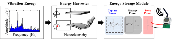
Figure 1. Concept of piezoelectric vibration energy harvesting to realize a self-powered wireless sensor.
Download figure:
Standard image High-resolution imageSince most ambient vibrations in nature are inherently random, the output electric power may also randomly change. Now, a question of fundamental importance arises how to explicitly elucidate the electroelastic behaviors of PVEH devices under random vibrations, and identify the key design parameters to carry out the enhanced output performance. With this purpose in mind, many researchers have sought to develop a stochastic electroelastically-coupled analytical model that provides a preliminary estimate the expected output electric power under 'stationary' random vibrations. Halvorsen [3] formulated a stochastic description of electroelastic modeling to calculate the expected output electric power. Adhikari et al [4] derived a closed form of a linear single degree of freedom model under white Gaussian noise. Ali et al [5] developed an equivalent linear model of a piezomagnetoelastic energy harvester under broadband random vibrations. Zhao et al [6] predicted the expected output electric power by employing a Fourier series representation or an Euler–Maruyama scheme to solve the stochastic differential equations under white Gaussian noise. Aridogan et al [7] presented electroelastic modeling and its experimental validation of a plate-like PVEH device from stationary random vibrations.
However, this type of analysis cannot readily answer a question about the 'nonstationarity' found in most realistic random vibrations. In general, when the statistical moments depend on the time, the random vibration signal is said to be nonstationary [8]. For instance, white Gaussian noise has a time-invariant power spectral density (PSD) over the entire frequency range, while nonstationary random vibrations have a time-variant PSD. There have been a few prior attempts to delve into both the 'nonstationarity' and the 'randomness' of an input excitation signal in PVEH analysis. Even though Seuaciuc-Osório and Daqaq [9] investigated the output performances of a PVEH device subject to harmonic excitations with a sinusoidally-varying frequency while keeping the acceleration level constant, such excitation cannot be considered random; rather, it is deterministic from a stochastic point of view. Recently, Yoon and Youn [10] proposed the stochastic electroelastically-coupled analytical model using time-frequency (TF) analysis to estimate the time-varying output electric power under nonstationary random vibrations. However, this study was not experimentally validated and did not cover the output mechanical performance, such as the displacement of the PVEH device.
The objective of this study is thus to lead to a deep understanding of the electroelastic behaviors of a PVEH device under nonstationary random vibrations through well-balanced correlation study of analytical prediction and experimental observation. The primary interest herein is to physically interpret the relationships between the time-varying output performances of the PVEH device and the two key loading parameters, including the operating frequency (i.e., the central frequency) and the electrical impedance (i.e., the external electrical circuit resistance). In this study, the central frequencies are selected to be off-resonance and near resonance for comparison, so that mechanical resonance effects are thoroughly investigated. The trends of the time-varying output performances of the PVEH device are examined with respect to various external electrical resistances under nonstationary random vibrations. The four-fold novel aspects of this study, compared to the previous work by Yoon and Youn [10], include:
- This study extends analytical investigation [10] by providing a well-designed 'experimental setup' to mimic realistic nonstationary random vibration signals and measure the time-varying output performances of a PVEH device.
- Rather than a pointwise validation, this study makes use of 'correlation metrics' to globally compare the predicted and measured results of the time-varying output performances of a PVEH device which to date have not been addressed in a deterministic approach.
- To the best of the authors' knowledge, this study is a pioneering work to investigate the effects of the central frequency of the input excitation signal ('mechanical resonance effects') and the external electrical resistance of the circuits ('electrical impedance effects') on the time-varying output performances of the PVEH device under nonstationary random vibrations.
- This study investigates the output mechanical (i.e., time-varying tip displacement) as well as electrical performances of a PVEH device.
The rest of this paper is organized as follows: section 2 describes the stochastic electroelastically-coupled analytical model using TF analysis. Section 3 presents an experimental design scheme for measuring the time-varying output performances of the PVEH device under nonstationary random vibrations. Thorough investigations on the effects of the central frequency and the external electrical resistance on the time-varying output performances of the PVEH are given in sections 4 and 5, respectively. Section 6 provides quantitative correlation analysis between the analytical and experimental results. Finally, the conclusions of this work are outlined in section 7.
2. Stochastic electroelastically-coupled analytical model using TF analysis
This section is devoted to a brief review of the stochastic electroelastically-coupled analytical model using TF analysis in our previous paper [10]. While we will mostly follow the description provided in [10], here we extend our previous model to a generalized framework that can estimate the time-varying tip displacement as well.
PVEH can be modeled as an electroelastic system that is linear and time-invariant, as depicted in figure 2. The randomness in both the single input excitation and the two output performances is taken into account in a stochastic manner, while all the parameters embedded in the electroelastic system are assumed to be exactly known and regarded as being deterministic. In this generalized framework, the input excitation signal x(t) is a nonstationary random vibration signal, and the output performances include both the output voltage v(t) and the tip displacement r(t).

Figure 2. Modeling of piezoelectric vibration energy harvesting as a linear and time-invariant electroelastic system with a single-input and two-outputs.
Download figure:
Standard image High-resolution imageCommon examples of the nonstationary random vibration signal include the following three types: amplitude-modulation (AM), frequency-modulation (FM), and AM-FM signals, as shown in figure 3. Since the input excitation signal x(t) is an acceleration with zero mean, the output performances, v(t) and r(t), also have zero mean. If the input excitation signal exhibits statistical regularity [8], it can be mathematically described in terms of a certain average, such as the time-variant PSD,  The bold–italic symbol denotes a complex-valued quantity in this study.
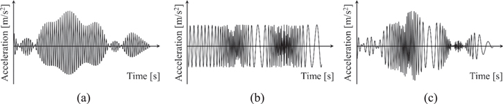
Figure 3. Common examples of nonstationary random vibrations: (a) amplitude-modulation, (b) frequency-modulation, and (c) amplitude- and frequency-modulation.
Download figure:
Standard image High-resolution imageIn figure 2, the frequency response function (FRF) for the output voltage,  and the FRF for the tip displacement,
  are the operators. These operators are used to define the linear relationships between the time-variant PSD of the input excitation signal,
  and those of the output voltage and the tip displacement,
  and
and  respectively. Note that the two FRFs may interact with each other due to the piezoelectric coupling. Finally, the linear relationships exhibited in stochastic dynamics of PVEH are expressed as:


Stochastic prediction of the time-varying output performances of PVEH devices consists of three sequentially executed procedures. The first step is to estimate the time-variant PSD of the input excitation signal,  by using TF analysis [10], such as the smoothed pseudo Wigner–Ville distribution (SPWVD) as:
where h and g denote the smoothing kernel windows.  is the Wigner–Ville distribution known to be an unbiased estimator for localization of an instantaneous frequency of the linear frequency-modulated signal with multiplicative noise [11].
The second step is to define the linear operators,  and
and  [10]. Many electroelastically-coupled analytical models have been previously developed based on the following the two governing equations, namely mechanical equation of motion and electrical circuit equation, respectively as [12]:
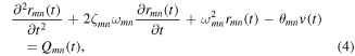

where the subscript mn represents the (m, n) vibration mode of a PVEH device. rmn(t) denotes the generalized mechanical coordinate and v(t) denotes the output voltage. Cp denotes the capacitance and Rload denotes the external electrical resistance.  denotes the modal mechanical damping ratio and
  denotes the natural angular frequency of the PVEH device.
  is referred to as the modal mechanical forcing function and
  denotes the modal electroelastic coupling. Under the assumption of a harmonic translational motion (vertical direction) for base excitation, the output voltage and the tip displacement can be expressed as
  and
and  respectively where j is the unit imaginary number. By substituting these exponential expressions into equations (4) and (5), amplitude of v(t) and r(t) can be solved as:
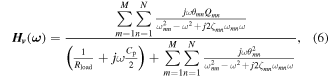
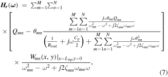
where Wmn(x, y) is the mode shape for a cantilever boundary condition. In equation (7), note that the FRF for the tip displacement is expressed in physical coordinates based on the modal expansion theorem. Ltip denotes the designated spot at which the relative displacement of the PVEH device is measured by a laser interferometer (near the tip of the cantilever). The detailed derivation procedure of electroelastically-coupled analytical models can be found in [12].
The third step is to estimate the time-variant PSDs of the output performances,  and
and  from the linear relationships in equations (1) and (2) [10]. Since an autocorrelation function,
  can be obtained by taking the inverse Fourier transform of a time-variant PSD, the mean square values of the output voltage and the tip displacement, E[v2(t)] and E[r2(t)], are estimated, respectively as:
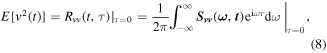
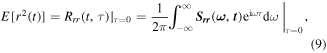
where E[•] denotes the statistical expectation. Therefore, amplitude of the time-varying output performances of the PVEH device can be calculated in a stochastic manner under nonstationary random vibrations.
3. Experimental design scheme for characterization of piezoelectric energy harvesting under nonstationary random vibrations
This section outlines an experimental design scheme for generating the input excitation signals with time-varying random characteristics and measuring the output performances of the PVEH device. Section 3.1 explains the experimental setup and section 3.2 describes the behavior of the input excitation signals in connection with key parameters, such as the central frequency and the electrical impedance.
3.1. Experimental setup
Figure 4 shows the experimental setup, which consists of five units: (1) actuation; (2) real-time monitoring of the input excitation signal; (3) measurement of the output electrical performance; (4) measurement of the output mechanical performance; and (5) data acquisition (DAQ). The actuation unit includes a function generator (Agilent, 35500B Series), a power amplifier (Bruel & Kjaer, Type 2718), and a vibration exciter/shaker (Bruel & Kjaer, Type 4809). Since the current of the signal produced by the function generator is not sufficient to drive the shaker, the power amplifier is used to increase the current of the signal. Then the shaker induces the input excitation signal x(t), which emulates realistic nonstationary random vibrations. In order to mount the PVEH device on the shaker, a clamping fixture is adopted. An accelerometer (Bruel & Kjaer, Type 4374 L) is attached to the clamping fixture to measure the real-time base acceleration as the input excitation signal. The output of the accelerometer is conditioned by a conditioning amplifier (Bruel & Kjaer, Type 2692) prior to entering one input channel of an oscilloscope (LeCroy, WaveRunner 604Zi). The oscilloscope is used to display the waveforms of the input excitation signal and the two output performances over time. To measure the output mechanical performance, a laser interferometer (Polytec, OFV-505, OFV-5000) is used to observe the absolute tip velocity of the PVEH device in the transverse direction relative to the fixed reference frame. Two of the remaining input channels of the oscilloscope are used for the output voltage and the absolute tip velocity. Finally, the oscilloscope is also used as a DAQ system to record all of the measurements as a function of time. The sampling frequency is 250 kHz for all monitoring and measurement.
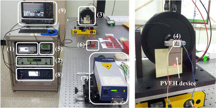
Figure 4. Experimental setup to excite/monitor the base acceleration and measure the output voltage and the absolute tip velocity. Unit 1: actuation: (1) function generator, (2) power amplifier, (3) shaker. Unit 2: real-time monitoring of the input excitation signal: (4) accelerometer, (5) conditioning amplifier. Unit 3: measurement of the output electrical performance: (6) external electric resistance. Unit 4: measurement of the output mechanical performance: (7) laser interferometer sensor head, (8) laser interferometer controller. Unit 5: data acquisition: (9) oscilloscope.
Download figure:
Standard image High-resolution imageFor a test specimen, this study used a commercially-available bimorph PVEH device (Piezo Systems Inc., T226-A4-503X) without a proof mass. Because the structural layer provides electrical conductivity, the outermost electrodes of the PVEH device are wired to the electrical circuit in a series connection. The input geometric dimensions and the material properties are listed in tables 1 and 2, respectively. The modal mechanical damping ratio  of the fundamental vibration mode at the short-circuit condition (electrically uncoupled) is identified as 0.026 518 in the experiment. The procedure to estimate the damping ratio is described in [13]. The fundamental resonance frequency f11 of the PVEH device is 106.78 Hz.
Table 1. Input geometric dimensions of the PVEH device.
| Thickness of piezoelectric layer |

|
0.27 mm |
| Thickness of the structural layer |

|
0.15 mm |
| Active length of the PVEH device |

|
54.25 mm |
| Width of the PVEH device |

|
31.78 mm |
Table 2. Input material properties of the PVEH device.
| Elastic modulus of structural layer |

|
100 GPa |
| Elastic modulus of piezoelectric layer |

|
66 GPa |
| Density of the piezoelectric layer |

|
7750 kg m−3 |
| Density of the structural layer |

|
7630 kg m−3 |
| Piezoelectric constant |

|
−10.40 C m−2 |
| Dielectric permittivity at constant strain |

|
13.30 nF m−1 |
3.2. Generation and analysis of input excitation random signals
In this study, the AM and AM-FM signals are considered as the input excitation signal x(t). The AM signal can be mathematically described as:

where  denotes the central amplitude and
  denotes the central angular frequency. For the AM signal, the instantaneous frequency is constant but the central amplitude is randomly modulated by the white Gaussian noise
  Therefore,
  denotes the acceleration level at a certain time t, which forms the wave envelope of the input excitation signal. On the other hand, the AM-FM signal can be mathematically described as:
where {2πfc + ε(t)} denotes the instantaneous angular frequency, which is the first derivative of the instantaneous phase. The instantaneous angular frequency is decomposed into the central frequency 2πfc and the frequency deviation that is described by the white Gaussian noise ε(t). For the AM-FM signal, the central frequency is the mean value of the instantaneous frequency.
For the purpose of systematically analyzing the time-varying output performances of the PVEH device at both off-resonances and near resonance, the central frequencies of the input excitation signal are selected to be 4, 60, and 90 (off-resonances), and 100 Hz (near resonance) for comparison. The external electrical resistance is fixed to 20 kΩ. Figure 5 shows the acceleration levels in the AM case, which are the 'wave envelopes' of the input excitation signal extracted by using the Hilbert transform [14]. The empty green rectangle indicates the instant time when the maximum acceleration level occurs in each case. For all cases, the maximum acceleration level is limited to about 5 m s−2. Figure 6 shows the acceleration level (black solid line) and the instantaneous frequency (blue dashed line) in the cases of AM-FM. The instantaneous frequency of the input excitation signal is extracted by using the Hilbert transform. The empty red circle indicates the time instant when the instantaneous frequency is closest to resonance (106.78 Hz).
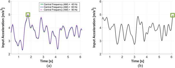
Figure 5. The acceleration levels of the input excitation signals in the AM case at central frequencies of: (a) 40, 60, and 90 Hz, and (b) 100 Hz.
Download figure:
Standard image High-resolution image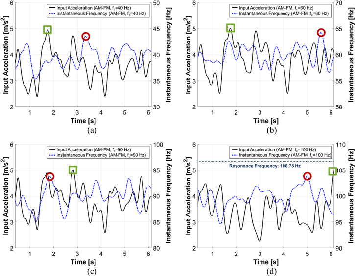
Figure 6. The acceleration levels and the instantaneous frequencies of the input excitation signals in the AM-FM case at central frequencies of: (a) 40 Hz, (b) 60 Hz, (c) 90 Hz, and (d) 100 Hz.
Download figure:
Standard image High-resolution imageFor the purpose of systematically analyzing the time-varying output performances of the PVEH device in terms of the electrical impedance, various external electrical resistances are selected to be 20 kΩ, 50 kΩ, 80 kΩ, 100 kΩ, 500 kΩ, and 1 MΩ for comparison. In this study, the external electrical resistance of 1 MΩ is considered as the open-circuit condition. For all cases, the central frequency is fixed as 90 Hz. Figure 7 shows the acceleration levels of the input excitation signals in the AM case with different electrical boundary conditions: 0 Ω (short-circuit condition), 20 kΩ, 100 kΩ, and 1 MΩ. For all cases, the maximum acceleration level is limited to about 5 m s−2. Figure 8 shows the acceleration level and the instantaneous frequency of the input excitation signals with the central frequency of 90 Hz in the case of AM-FM. It is worth pointing out that the input excitation signal at the short-circuit condition is essentially the same as the cases in which the external electrical resistances are 20 kΩ, 100 kΩ, and 1 MΩ in the AM and AM-FM cases. This implies that the external electrical resistance has little effect on the mounting clamp dynamics and its interaction with the shaker.
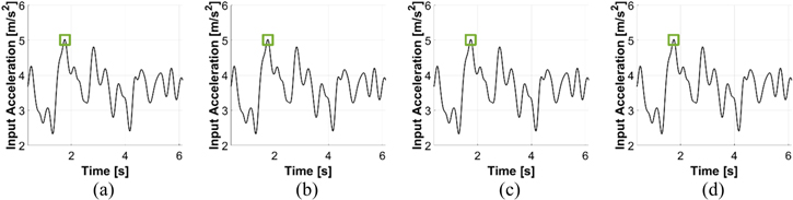
Figure 7. The acceleration levels of the input excitation signals in the AM case at the external electrical resistance of: (a) 0 kΩ (short-circuit), (b) 20 kΩ, (c) 100 kΩ, and (d) 1 MΩ.
Download figure:
Standard image High-resolution image
Figure 8. The acceleration levels and the corresponding instantaneous frequencies of the input excitation signals in the AM-FM case at the external electrical resistance of: (a) 0 kΩ (short-circuit), (b) 20 kΩ, (c) 100 kΩ, and (d) 1 MΩ.
Download figure:
Standard image High-resolution image4. Effects of the central frequency on the time-varying output performances of a PVEH device under nonstationary random vibrations
The objective of this section is to understand how the central frequency of input nonstationary random vibrations affects the time-varying output performances of a PVEH device. Section 4.1 investigates the time-varying output performances of a PVEH device subject to AM signals (figure 5), while AM-FM signals (figure 6) are considered in section 4.2.
4.1. Performance in the AM case
In figure 9, the wave envelopes of the measured output voltage are graphically compared with the analytical results in the time domain in the AM case. The wave envelopes of the measured output voltage were extracted by using the Hilbert transform. Recall that the external electrical resistance is set to 20 kΩ for all cases. Comparison of figures 5 and 9 clearly suggests a direct proportional relationship between the acceleration level and the corresponding output voltage when the operating frequency remains constant. In addition, it is observed that the magnitude of the wave envelope of the time-varying output voltage increases, as the central frequency varies from 40 to 100 Hz as it gets closer to the resonance frequency of 106.78 Hz. In experiment, the maximum magnitude of the time-varying output voltage is about 2.19 V at the central frequency of 100 Hz when the acceleration level is approximately 4.97 m s−2 at t = 6.12 s, as shown in figure 9(d).
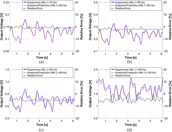
Figure 9. The predicted versus measured output voltage in the AM case at central frequencies of: (a) 40 Hz, (b) 60 Hz, (c) 90 Hz, and (d) 100 Hz.
Download figure:
Standard image High-resolution imageThe dashed black lines indicate the relative error (RE) at a certain time ti, which is calculated as:

A positive relative error means that the value of the predicted wave envelope is higher than the measured one, thereby indicating overestimation. In contrast, a negative relative error represents underestimation. Overall, analytical prediction is in a good agreement with experimental observation for the time-varying output voltage. In figure 9, at the central frequency of 40 Hz (off-resonance), analytical prediction and experimental observation align well (the magnitude of the relative error is below 1.87%), because the PVEH device is effectively being operated away from resonance. On the other hand, at the central frequency of 100 Hz (near resonance), the discrepancy between the predicted and measured results is pronounced (the magnitude of the relative error is below 7.39%), because a relatively large mechanical strain is applied. This implies that the deviation occurring near resonance is mainly attributed to the nonlinearity that is not incorporated in analytical prediction. Despite the local discrepancy, the stochastic electroelastically-coupled analytical model well captures the trend of the wave envelope of the measured time-varying output voltage for all the AM cases.
In figure 10, the wave envelopes of the tip displacement taken in the experiment are graphically compared with the analytical results in the AM case. The wave envelope of the time-varying tip displacement increases as the central frequency gets closer to the resonance frequency of the PVEH device. From figure 10, it is also confirmed that the wave envelope of the time-varying tip displacement depends on the acceleration level only in the AM case. In experiment, the maximum magnitude of the time-varying tip displacement is about 102.61 μm at the central frequency of 100 Hz when the acceleration level is about 4.97 m s−2 at t = 6.12 s, as shown in figure 10(d). It is observed that the mean values of the relative error are approximately 4.68%, 5.39%, 0.93%, and 2.61% at the central frequencies of 40 Hz, 60 Hz, 90 Hz, and 100 Hz, respectively. Therefore, overall, analytical prediction is in a good agreement with experimental observation for the time-varying tip displacement of the PVEH device.

Figure 10. Predicted versus measured tip displacement in the AM case at central frequencies of: (a) 40 Hz, (b) 60 Hz, (c) 90 Hz, and (d) 100 Hz.
Download figure:
Standard image High-resolution imageIt is worth noting that the absolute values of the relative error are momentarily high at the instant when the envelopes of the time-varying output performances are at the local extrema. There can be two main sources of the local discrepancy. First, in analytical prediction, the resolution of the smoothing kernel window in the SPWVD could be insufficient to capture a rapidly varying amplitude of the input excitation signal. However, the resolution issue can be improved by optimizing the size of the smoothing kernel window. The other possible reason is that the Hilbert transform could introduce a bias when extracting the wave envelope of the measured time-varying output performances. The original waveforms of the measured time-varying output performances and their envelopes have common tangents at contact points. The contact points of the envelopes do not exactly correspond to the local extrema (peak value) of the original waveforms [14]. Because the stochastic electroelastically-coupled analytical model estimates the peak values of the time-varying output performances at a certain time, the local discrepancy could occur due to a mismatching of these contact points.
The left, middle, and right columns of figure 11 show the time-variant PSDs of the input excitation signal, the output voltage, and the tip displacement, respectively, in the AM case. This study used a Hann window for the smoothing kernel windows in the SPWVD. Since the frequency content of the input excitation signal is a monocomponent, the time-variant PSD is a single-delineated region of the signal energy localization along a straight line in the TF plane. The shape and magnitude of the time-variant PSD of the input excitation signal are determined by the acceleration level only. The shape of the time-variant PSDs of the output performances is the same as that of the input excitation signal. However, it is worth pointing out that the magnitude of the time-variant PSDs of the output performances sharply increases, even though the magnitude of the time-variant PSD of the input excitation signal does not change, as the central frequency approaches to 100 Hz.

Figure 11. Time-variant PSDs of the input excitation signal, the output voltage, and the tip displacement for the AM case at central frequencies of: (a) 40 Hz, (b) 60 Hz, (c) 90 Hz, and (d) 100 Hz.
Download figure:
Standard image High-resolution image4.2. Performance in the AM-FM case
Figure 12 shows the time-varying output voltage in the AM-FM case. The external electrical resistance is set to 20 kΩ. In experiment, at the central frequency of 40 Hz (off-resonance), comparison of figures 6(a) and 12(a) shows that the maximum output voltage of 0.17 V is achieved when the maximum acceleration level of 4.96 m s−2 at t = 1.75 s. At the central frequency of 100 Hz (near resonance), however, comparison of figures 6(d) and 12(d) shows that the maximum acceleration level of 4.96 m s−2 at t = 6.12 s does not guarantee the generation of the maximum output voltage. Rather, the maximum output voltage of 2.21 V is observed when the acceleration level and the instantaneous frequency are 2.86 m s−2 and 103.78 Hz at t = 5.02 s, respectively. This is attributed to the fact that the PVEH device is designed as a resonator. It can be thus concluded that, near resonance, a closer distance between the instantaneous frequency and the resonance frequency ensure the higher generation of the time-varying output voltage, if the acceleration level is the same.

Figure 12. The predicted versus measured output voltage in the AM-FM case at central frequencies of: (a) 40 Hz, (b) 60 Hz, (c) 90 Hz, and (d) 100 Hz.
Download figure:
Standard image High-resolution imageIn cases of off-resonance, the predicted time-varying output voltage is in an excellent agreement with the measured one. As shown in figures 12(a)–(c), the relative error is below 5.36%. In the case of near resonance, it is worth noticing that the discrepancy between analytical prediction and experimental observation is relatively large where the relative error is 18.61% at t = 5.02 s, as shown in figure 12(d). As indicated by the empty red circle in figure 6(d), the instantaneous frequency of the input excitation signal comes close to the resonance frequency of the PVEH device at t = 5.02 s. Near resonance, a small driving force may cause relatively large deformations of the PVEH device. This inherent nonlinear effect could greatly affect the output performances of the PVEH device. Indeed, the electroelastically-coupled analytical model based on the linear constitutive relations for piezoelectricity has limited predictive capability for estimation of the output performance of the PVEH device near resonance due to nonlinear effects of large deformations [15]. It has been reported that the output voltage predicted by the electroelastically-coupled analytical model under a linear assumption could be underestimated relative to the experimental observation near resonance when the nonlinearity in the piezoelectric coupling is moderate [16]. In addition, the actual value of the piezoelectric constant exhibits significant dependence on the mechanical strain induced in the piezoelectric layer [16]. The experimentally measured data of the piezoelectric constant increases with the induced strain [17], while the linear model assumes it remains unchanged. Nonlinear PVEH is beyond the scope of this study; details can be found in [18].
Figures 13(a)–(d) show the time-varying tip displacement in the AM-FM case. As expected, the trend of the overall envelope of the time-varying tip displacement is similar to that of the time-varying output voltage. In experiment, at the external electrical resistance of 20 kΩ, the maximum magnitude of the time-varying tip displacement is about 93.10 μm when the acceleration level and the instantaneous frequency are 2.86 m s−2 and 103.78 Hz at t = 5.02 s, respectively, as shown in figure 13(d). The maximum relative error of 12.06% occurs at t = 5.02 s.
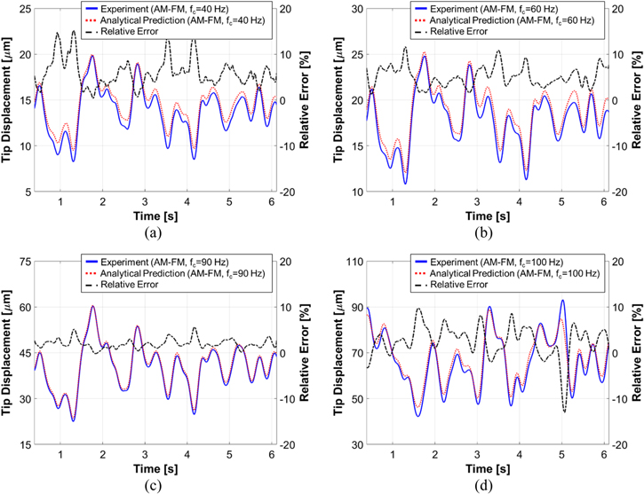
Figure 13. The predicted versus measured tip displacement in the AM-FM case at central frequencies of: (a) 40 Hz, (b) 60 Hz, (c) 90 Hz, and (d) 100 Hz.
Download figure:
Standard image High-resolution imageThe left, middle, and right columns of figure 14 describe the time-variant PSDs of the input excitation signal, the output voltage, and the tip displacement, respectively, in the AM-FM case. As shown in the left column of figure 14, the shape and magnitude of the time-variant PSD of the input excitation signal are determined by the acceleration level. However, unlike the AM case, the single-delineated region of the signal energy localization is not fixed along a straight line; instead, it changes with the operating frequency in the TF plane. In the AM-FM case, even when the acceleration level of the input excitation signal is high at a certain time, the time-variant PSDs of the output performances can be relatively low if the operating frequency is far from resonance.
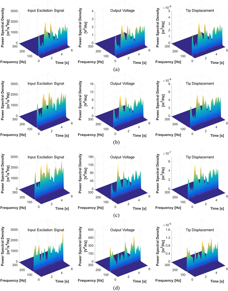
Figure 14. Time-variant PSDs of the input excitation signal, the output voltage, and the tip displacement in the AM-FM case at central frequencies of: (a) 40 Hz, (b) 60 Hz, (c) 90 Hz, and (d) 100 Hz.
Download figure:
Standard image High-resolution imageAlteration of the spectral characteristics of the input excitation signal can be attributed entirely to the electroelastically-coupled FRFs of the PVEH device, which are defined as the linear operators in section 2. The linear operators prescribe the amount of energy transmitted by the electroelastic system at various operating frequencies. Equations (1) and (2) account for the fact that the electroelastic system has the effect of modulating the shape of the time-variant PSD of the input excitation signal. This electroelastic behavior becomes more remarkable as the central frequency gets closer to the resonance frequency of the PVEH device. In fact, the shape of time-variant PSD of the input excitation signal is almost the same as that of the output performances of the PVEH device at a central frequency of 40 Hz, which is quite far from resonance. However, figures 14(b)–(d) clearly show that the shapes of time-variant PSDs of the output performances are different from those of the input excitation signals at central frequencies of 60–100 Hz. In the AM-FM cases, a key finding is thus that, rather than the acceleration level, the degree of off-resonance dominantly affects the time-varying output performances of the PVEH device. Because the operating frequency changes over time under nonstationary random vibrations, this time-variant spectrum of the output performances of the PVEH device is a primary feature; it has not been addressed under deterministic harmonic excitations or even stationary random vibrations.
5. Effects of the electrical impedance on the time-varying output performances of a PVEH device under nonstationary random vibrations
This section explores the effect of the electrical impedance of circuits on the time-varying performances of PVEH devices under nonstationary random vibrations. Section 5.1 investigates the time-varying output performances of a PVEH device subject to AM signals (figure 7(a)). AM-FM signals (figure 7(b)) are considered in section 5.2.
5.1. Performance in the AM case
Figure 15 shows the time-varying output voltage across various external electrical resistances subject to AM signals. The central frequency is 90 Hz. As shown in figures 15(a)–(f), the asymptotic behavior of the wave envelope of the time-varying output voltage can be found with respect to the external electrical resistance. The magnitude of the wave envelope of the time-varying output voltage monotonically rises as the external electrical resistance approaches the open-circuit condition. Following a certain value of the external electrical resistance, the magnitude of the wave envelope of the time-varying output voltage converges to the maximum. In experiment, comparison of figures 7 and 15 shows that the maximum magnitude of the time-varying output voltage is about 1.81 V at the external electrical resistance of 1 MΩ when the acceleration level is approximately 5.02 m s−2 at t = 1.75 s. Overall, analytical prediction of the time-varying output voltage is in a great agreement with experimental observation at different external electrical resistances. Interestingly, even though the magnitude of the relative error increases as the external electrical resistance approaches the open-circuit condition, its trend over time remains almost unchanged. Except for the external electrical resistance of 20 kΩ, the stochastic electroelastically-coupled analytical model slightly overestimates the wave envelopes of the time-varying output voltage compared to the measurement. This overestimation becomes somewhat larger when the external electrical resistance increases. As the predicted and measured values of the time-varying output voltage asymptotically converge, so does the magnitude of the relative error. In figure 15(f), the magnitude of the relative error for the time-varying output voltage ranges from 6.46% to 10.09% at the external electrical resistances of 1 MΩ.
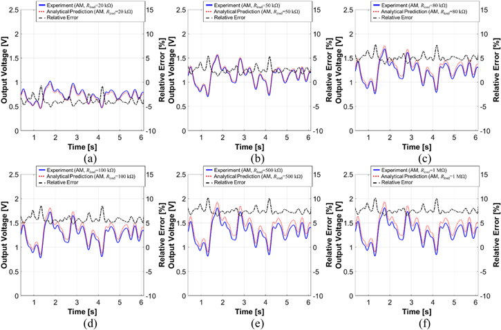
Figure 15. The predicted versus measured output voltage across the external electrical resistances of: (a) 20 kΩ, (b) 50 kΩ, (c) 80 kΩ, (d) 100 kΩ, (e) 500 kΩ, and (f) 1 MΩ in the AM case.
Download figure:
Standard image High-resolution imageFigure 16 shows the time-varying tip displacement at various external electrical resistances subject to AM signals. In experiment, comparison of figures 7 and 16 shows that the maximum magnitude of the time-varying tip displacement is about 52.29 μm at the external electrical resistance of 20 kΩ when the acceleration level is approximately 5.03 m s−2 at t = 1.75 s. As the predicted and measured values of the tip displacement asymptotically converge, so does the magnitude of the relative error. In figure 16(f), the magnitude of the relative error ranges from 2.09% to 6.75% at the external electrical resistance of 1 MΩ. For all of external electrical resistances, analytical prediction is mostly in a good agreement with experimental observation in the AM case. It is worth pointing out that the tip displacement decreases below resonance with increasing in the external electrical resistance, while it increases in the vicinity of anti-resonance [19]. As the operating frequency increases towards resonance, the decrement of the tip displacement becomes greater although it is not proportional to the external electrical resistance. Because the operating frequency of the input excitation signal is 90 Hz (off-resonance), the magnitude of the tip displacement monotonically decreases as the external electrical resistance increases toward the open-circuit condition. This gradual attenuation of the tip displacement with increasing the external electrical resistance is associated with a gradual increase in the output voltage [20]. Following a certain value of the external electrical resistance, the tip displacement converges to the minimum at the corresponding acceleration level.
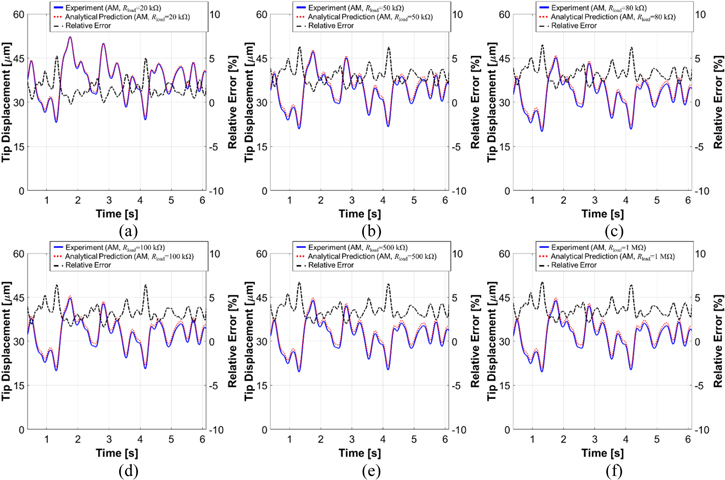
Figure 16. The predicted versus measured tip displacement at the external electrical resistances of: (a) 20 kΩ, (b) 50 kΩ, (c) 80 kΩ, (d) 100 kΩ, (e) 500 kΩ, and (f) 1 MΩ in the AM case.
Download figure:
Standard image High-resolution imageFigures 17 and 18 show the asymptotic tendency of the time-variant PSDs of the output performances with respect to the external electrical resistance in the AM case. From equations (6) and (7), one can notice that the external electrical resistance is included as a variable in the electroelastically-coupled FRFs. The magnitude of the time-variant PSDs of the output voltage monotonically increases as the external electrical resistance increases. After that, the time-variant PSDs of the output voltage converge to a certain value as the external electrical resistance tends to the open-circuit condition. The magnitude of the time-variant PSDs of the tip displacement monotonically decreases as the external electrical resistance approaches the open-circuit condition.

Figure 17. Time-variant PSDs of the output voltage in the AM case. The external electrical resistances are: (a) 20 kΩ, (b) 50 kΩ, (c) 80 kΩ, (d) 100 kΩ, (e) 500 kΩ, and (f) 1 MΩ.
Download figure:
Standard image High-resolution image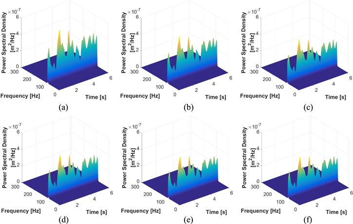
Figure 18. Time-variant PSDs of the tip displacement in the AM case. The external electrical resistances are: (a) 20 kΩ, (b) 50 kΩ, (c) 80 kΩ, (d) 100 kΩ, (e) 500 kΩ, and (f) 1 MΩ.
Download figure:
Standard image High-resolution image5.2. Performance in the AM-FM case
Figures 19 and 20 show the time-varying output voltage and the tip displacement at various external electrical resistances in the AM-FM case, respectively. The central frequency is 90 Hz. Because the operating frequency randomly changes, the wave envelope of the time-varying output performances depends on both the acceleration level and the operating frequency in figure 7(b). In experiment, comparison of figures 8 and 19 shows that the maximum magnitude of the time-varying output voltage is 2.05 V across the external electrical resistance of 1 MΩ when the acceleration level is 4.88 m s−2 and the instantaneous frequency is 93.35 Hz at t = 1.77 s. As shown in figure 20, the maximum magnitude of the time-varying tip displacement is 59.89 μm at the external electrical resistance of 20 kΩ.
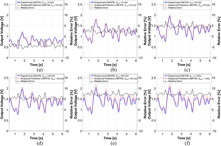
Figure 19. The predicted versus measured output voltage across the external electrical resistances of: (a) 20 kΩ, (b) 50 kΩ, (c) 80 kΩ, (d) 100 kΩ, (e) 500 kΩ, and (f) 1 MΩ in the AM-FM case.
Download figure:
Standard image High-resolution image
Figure 20. The predicted versus measured tip displacement across external electrical resistances of: (a) 20 kΩ, (b) 50 kΩ, (c) 80 kΩ, (d) 100 kΩ, (e) 500 kΩ, and (f) 1 MΩ in the AM-FM case.
Download figure:
Standard image High-resolution imageThe asymptotic behavior of the wave envelope of the time-varying output performances can be also found with respect to external electrical resistance in the AM-FM. The magnitude of the wave envelope of the time-varying output voltage increases with increasing the external electrical resistance, while that of the time-varying tip displacement decreases, because the operating frequency of the input excitation signals is off-resonance. However, the external electrical resistance has no effect on to the trend of the wave envelope of the output performances, as was seen for the AM case. For all various external electrical resistances, the predicted envelopes of the time-varying output performances are in a good agreement with the measured ones in the AM-FM case. In figure 19(f), the magnitude of the relative error for the time-varying output voltage ranges from 6.25% to 9.53% under the open-circuit condition. In figure 20(f), the magnitude of the relative error for the time-varying tip displacement ranges from 1.82% to 5.76% at the external electrical resistance of 20 kΩ.
Figures 21 and 22 show the time-variant PSDs of the output voltage and the tip displacement, respectively, at various external electrical resistances subject to an AM-FM signal. The asymptotic behaviors of the time-variant PSDs of the output performances can be clearly found as the external electrical resistance increases toward the open-circuit condition. Like the AM case, the external electrical resistance is only contributory to the magnitude of the time-variant PSDs of the output performances, as shown in figures 21 and 22. For the AM-FM signal, since the central frequency is the mean value of the instantaneous frequency, it is recommended that, as a preliminary step, the external electrical resistance be fixed to be the optimal value suitable for the central frequency. Note that in a view of a practical application, nonlinear circuit techniques for load-independent energy harvesting are required [21, 22], since the electrical impedance could be changed according to power-consuming conditions (i.e., work- or sleep-modes of wireless sensor nodes).
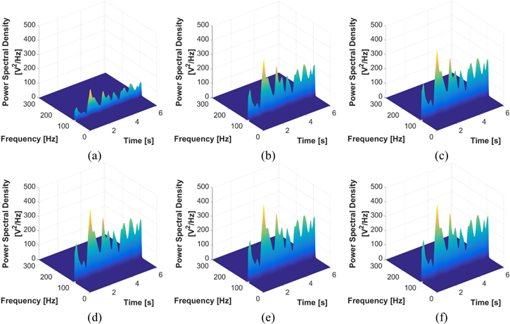
Figure 21. Time-variant PSDs of the output voltage in the AM-FM case. External electrical resistances are: (a) 20 kΩ, (b) 50 kΩ, (c) 80 kΩ, (d) 100 kΩ, (e) 500 kΩ, and (f) 1 MΩ.
Download figure:
Standard image High-resolution image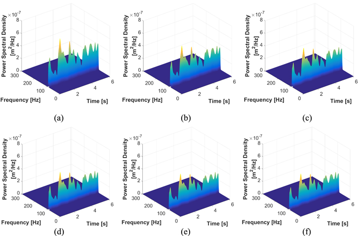
Figure 22. Time-variant PSDs of the tip displacement in the AM-FM case. External electrical resistances are: (a) 20 kΩ, (b) 50 kΩ, (c) 80 kΩ, (d) 100 kΩ, (e) 500 kΩ, and (f) 1 MΩ.
Download figure:
Standard image High-resolution image
6. Quantitative correlation analysis between prediction and measurement
This section is devoted to providing quantitative correlation analysis for comparing the predicted and measured results. This quantitative correlation analysis was performed for the 'wave envelopes' of the time-varying output performances of the PVEH device. Section 6.1 briefly summarizes several correlation metrics suitable for assessing the predictive capability of the stochastic electroelastically-coupled analytical model for the time-varying output performances of a given PVEH system; analysis results are given in section 6.2.
6.1. Summary of correlation metrics
In equation (13), xi denotes the entity of the envelope vector X of the predicted time-varying output performance of the PVEH device at a certain time ti, while yi denotes the entity of the envelope vector Y of the measured performance, as:

where k denotes the sample size of the envelope vector. The sample size of the envelope vector is determined by the sampling rate. It is helpful to evaluate the magnitude error and the phase error by using an aggregate measure. With that purpose, in this work, the degree of the discrepancy between the time histories is assessed in a three-fold manner as: (1) the normalized root mean square error (NRMSE); (2) the correlation coefficient; and (3) the weighted integrated factor (WIFac).
First, the NRMSE is defined as:

If the value of the NRMSE is close to 0, it can be concluded that analytical prediction is highly accurate. Therefore, the NRMSE provides a useful measure to assess the difference in magnitudes between analytical prediction and experimental observation. The major limitation of the NRMSE is that it is hard to provide information on the phase error.
Second, the correlation coefficient indicates the degree of the linear relationship between the two time histories, denoted by  which can be calculated as:

where σX and σY denote the standard deviations of the two time histories. The correlation coefficient is closely related to the phase error. For instance, if the correlation coefficient is close to 1.0, the wave envelopes of the predicted and measured output performances have the same phase as each other.
Third, the WIFac is a value weighted by the absolute maximum of the predicted and measured envelopes of the time-varying output performances X and Y as:
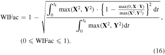
This weighting has the effect of scaling local differences to increase the effect of errors at high magnitude function values. The advantage of the WIFac is the ability to quantify the combined effects of the magnitude error and the phase error. As the value of the WIFac gets closer to 1.0, it indicates that the wave envelope of the predicted time-varying output performance is in a greater agreement with the measured one in terms of both the magnitude and the phase.
6.2. Error analysis results
Table 3 shows that the values of the correlation coefficient and the WIFac are very close to 1.000, and the values of the NRMSE are less than 0.078. As the central frequency of the input excitation signal is further away from the resonance frequency of the PVEH device, the discrepancy in the magnitude becomes smaller and, thereby, the value of the NRMSE gets closer to zero. The correlation coefficients are equal to 1.000 at the central frequencies of 40, 60, and 90 Hz in both the AM and AM-FM cases. However, it is worth pointing out that the correlation coefficient is 0.986 at the central frequency of 100 Hz in the AM-FM case, while it is very close to 1.000 in the AM case. Due to the combined effects of the errors in the local trend and in the magnitude, the value of the WIFac at the central frequency of 100 Hz is relatively smaller than that of the other central frequencies in the AM-FM case. In table 4, the values of the correlation coefficient and the WIFac are above 0.985 and 0.947, respectively, and the values of the NRMSE are below 0.067 for the time-varying tip displacement. Therefore, the error analysis results reveal that the predicted output performances of the PVEH device are in a very good agreement with the measured ones at various central frequencies.
Table 3. Error analysis results for the time-varying output voltage at various central frequencies. The external electrical resistance is 20 kΩ.
| 40 Hz | 60 Hz | 90 Hz | 100 Hz | ||
|---|---|---|---|---|---|
| Amplitude modulation (AM) | Normalized root mean square error (NRMSE) | 0.015 | 0.030 | 0.070 | 0.078 |
| Correlation coefficient | 1.000 | 1.000 | 1.000 | 0.997 | |
| Weighted integrated factor (WIFac) | 0.989 | 0.978 | 0.947 | 0.951 | |
| Amplitude and frequency modulation (AM-FM) | Normalized root mean square error (RMSE) | 0.012 | 0.034 | 0.039 | 0.077 |
| Correlation coefficient | 1.000 | 1.000 | 1.000 | 0.986 | |
| Weighted integrated factor (WIFac) | 0.991 | 0.973 | 0.961 | 0.938 | |
Table 4. Error analysis results for the time-varying tip displacement at various central frequencies. The external electrical resistance is 20 kΩ.
| 40 Hz | 60 Hz | 90 Hz | 100 Hz | ||
|---|---|---|---|---|---|
| Amplitude modulation (AM) | Normalized root mean square error (NRMSE) | 0.054 | 0.067 | 0.013 | 0.044 |
| Correlation coefficient | 1.000 | 1.000 | 1.000 | 0.997 | |
| Weighted integrated factor (WIFac) | 0.957 | 0.951 | 0.990 | 0.973 | |
| Amplitude and frequency modulation (AM-FM) | Normalized root mean square error (NRMSE) | 0.067 | 0.064 | 0.021 | 0.054 |
| Correlation coefficient | 0.999 | 0.996 | 0.999 | 0.985 | |
| Weighted integrated factor (WIFac) | 0.947 | 0.953 | 0.981 | 0.960 | |
Table 5 shows that the correlation coefficients are equal to 1.000, while the values of the WIFac are above 0.931 and those of the NRMSE are below 0.099 for the time-varying output voltage across various external electrical resistances. This implies that the trends of the predicted and measured envelopes of the time-varying output voltage remain almost unchanged regardless of the external electrical resistance. In the AM case, it is observed that the NRMSE increases as the external electrical resistance increases, ranging from 0.032 at 50 kΩ toward 0.099 at 1 MΩ. Since the correlation coefficients are equal to 1.000, it can be concluded that the magnitude error is a major cause that lowers the WIFac in the AM case as the external electrical resistance increases. One can notice that the values of both the NRMSE and the WIFac converge asymptotically. For the time-varying tip displacement at various external electrical resistances, table 6 shows that the correlation coefficients are equal to 1.000, while the values of the WIFac are above 0.967 and those of the NRMSE are below 0.045 in the AM case. In the AM-FM case, the correlation coefficients are above 0.997, while the values of the WIFac are above 0.971 and those of the NRMSE are below 0.034. The asymptotic convergence of the NRMSE and the WIFac can be observed for the time-varying tip displacement as the external electrical resistance increases from 50 kΩ to 1 MΩ. The error analysis results reveal that the predicted output performances are in a very good agreement with the measured ones at various external electrical resistances.
Table 5. Error analysis results for the time-varying output voltage across various external electrical resistances. The central frequency is 90 Hz.
| 20 kΩ | 50 kΩ | 80 kΩ | 100 kΩ | 500 kΩ | 1 MΩ | ||
|---|---|---|---|---|---|---|---|
| Amplitude modulation (AM) | Normalized root mean square error (NRMSE) | 0.054 | 0.032 | 0.066 | 0.075 | 0.098 | 0.099 |
| Correlation coefficient | 1.000 | 1.000 | 1.000 | 1.000 | 1.000 | 1.000 | |
| Weighted integrated factor (WIFac) | 0.989 | 0.976 | 0.953 | 0.947 | 0.932 | 0.931 | |
| Amplitude and frequency modulation (AM-FM) | Normalized root mean square error (NRMSE) | 0.045 | 0.025 | 0.051 | 0.060 | 0.080 | 0.081 |
| Correlation coefficient | 1.000 | 1.000 | 1.000 | 1.000 | 1.000 | 1.000 | |
| Weighted integrated factor (WIFac) | 0.955 | 0.977 | 0.956 | 0.949 | 0.934 | 0.933 | |
Table 6. Error analysis results for the time-varying tip displacement at various external electrical resistances. The central frequency is 90 Hz.
| 20 kΩ | 50 kΩ | 80 kΩ | 100 kΩ | 500 kΩ | 1 MΩ | ||
|---|---|---|---|---|---|---|---|
| Amplitude modulation (AM) | Normalized root mean square error (NRMSE) | 0.020 | 0.038 | 0.041 | 0.041 | 0.044 | 0.045 |
| Correlation coefficient | 1.000 | 1.000 | 1.000 | 1.000 | 1.000 | 1.000 | |
| Weighted integrated factor (WIFac) | 0.985 | 0.972 | 0.970 | 0.970 | 0.968 | 0.967 | |
| Amplitude and frequency modulation (AM-FM) | Normalized root mean square error (NRMSE) | 0.016 | 0.030 | 0.032 | 0.032 | 0.033 | 0.034 |
| Correlation coefficient | 0.998 | 0.998 | 0.998 | 0.998 | 0.997 | 0.997 | |
| Weighted integrated factor (WIFac) | 0.986 | 0.974 | 0.972 | 0.972 | 0.971 | 0.971 | |
7. Conclusion
The main objective of this study was to explore the time-varying output performances of a PVEH device both analytically and experimentally under nonstationary random vibrations, considering the effects of the central frequency and the external electrical resistance. It was demonstrated that a larger acceleration level and a closer distance between the operating frequency and the resonance frequency of the PVEH device ensure higher generation of the time-varying output voltage. The magnitude of the wave envelope of the time-varying output performances shows the asymptotic tendency with increasing the external electrical resistance. The quantitative correlation analysis reveals that the predicted results are in an excellent agreement with the experimental observations both mechanically and electrically. Near resonance, however, the discrepancy between the predicted and measured results is momentarily large due to the nonlinear relationship between the applied strain and the electric field of the piezoelectric layer. Furthermore, the discrepancy increases as the external electrical resistance approaches the open-circuit condition.
Future work will incorporate structural and piezoelectric coupling nonlinearities into the stochastic electroelastically-coupled analytical model so as to further reduce the discrepancy between the predicted and measured time-varying output performances near resonance. Meanwhile, the nonstationary random vibration signals considered in this study—referred to as a monocomponent signals—have a slow-varying amplitude and a slow-varying always positive instantaneous frequency. Many practical nonstationary random vibration signals with a wideband spectrum can be considered as a multicomponent signal representing the sum of two or more monocomponent signals. Future work will thus include investigation of the effects of higher-order vibration modes on the time-varying output performances under wideband random vibration signals (e.g., a multicomponent AM-FM signal).
Acknowledgments
This research was supported by the National Research Council of Science & Technology (NST) grant by the Korea Government (MSIT) (No. CAP-17-04-KRISS); the Technology Innovation Program (10050980, System Level Reliability Assessment and Improvement for New Growth Power Industry Equipment) funded by the Ministry of Trade, Industry & Energy (MI, Korea); and funded by Korea Research Institute of Standards and Science (KRISS-2017-GP2017-0018).