

Abstract
In the past two decades, the aerospace industry has massively shifted from aluminum-made components to composite materials such as carbon fiber reinforced polymers (CFRP), striving for more fuel efficient and lighter aircrafts. Consequently, traditional joints have been replaced by adhesive bonded interfaces, which are also the most common choice to repair damaged components. Although adhesive bonding is the most efficient choice for permanent connections, it is not free of disadvantages: one of the most common failure modes, the debonding of the two laps, is very problematic to detect and predict in practice. Therefore, frequent inspections must be performed to ensure structural safety, increasing maintenance costs, and lessening the availability of the platforms. The development of innovative sensing technologies has allowed for a close monitoring of structural interfaces, and several structural health monitoring techniques have been proposed to monitor adhesive bonded connections. Sensitivity and correlation between measurements and debonding entity has been demonstrated in the literature: nevertheless, hardly any technique has been proposed and quantitively evaluated to estimate the debonding entity independently of the applied loads, such as misalignment-induced torsion, which is a major confounding influence in the traditional backface strain gauge technique. This paper proposes the inverse finite element method (iFEM) as a load and material independent approach to infer the debonding entity from strain measurements in adhesive-bonded joints. Two approaches to estimate the debonding entity with the iFEM are compared on cracked leap shear specimens representative of CFRP repair patches: one is based on anomaly indexes, the other on performing a model selection with multiple iFEM models including different damages. The latter demonstrates satisfactory performances; thus, it is considered a significant scientific advancement in this field.
Export citation and abstract BibTeX RIS

Original content from this work may be used under the terms of the Creative Commons Attribution 4.0 license. Any further distribution of this work must maintain attribution to the author(s) and the title of the work, journal citation and DOI.
1. Introduction
In the past decades, the aerospace industry has undergone a massive transition to achieve lighter and stronger structures, leading to the widespread employment of composite materials such as carbon fiber reinforced polymers (CFRP) in structural frames [1–3]. However, two of the main issues of composite materials are the connection and interfaces between the components and the repairability of the components themselves. Although joints are usually the most critical elements in any structure, in the case of composite materials they represent a significant burden since traditional methods such as mechanical fastening are terribly inefficient with composites [4]. One of the most efficient strategy to join two composite parts is to bond them through an adhesive; this technique is known as adhesive bonding [5], and it can be considered the golden standard in the aerospace sector, given that adhesive bonded joints are more aerodynamically efficient, lighter, and they guarantee higher thermal and electrical insulation and damping than discontinuous connections; last but not least, they redistribute the load more evenly, avoiding stress concentration typical of mechanical fastening [4]. Moreover, adhesive-bonded patches are also the preferable choice in repairing composite structures [6] since they can restore the original stiffness and strength of a damaged structure. However, adhesive bonding is not free of disadvantages: the adhesive material is typically very sensitive to environmental factors [7], such as temperature variations or corrosion, and adhesive-bonded interfaces are challenging to inspect [5, 8]. Despite the load being evenly distributed in an adhesive-bonded connections, the stress distribution in the interface is nonuniform, which causes one of the main failure modes for an adhesive-bonded interface: the debonding of the two laps, which is very problematic to predict in practice [9]. Therefore, frequent and thorough inspections have to be carried out on such components while in service, reducing the availability of the platforms and increasing the maintenance costs.
The development of innovative sensing technologies, such as distributed fiber optic strain measurements, has allowed a close interrogation of structural interfaces [10], aiming to the development of damage-tolerant structures and structural interfaces that embed sensors so that the structural health status can be monitored, in a framework that is known as structural health monitoring (SHM) [11]. Relevant research has been devoted to developing techniques to assess the structural integrity of adhesive bonded joints and composite repair patches.
In [12], the authors compared the performances of external and scarfed bonded repair patches, monitoring their behavior by means of ultrasonic guided waves, also known as Lamb waves, and digital image correlation (DIC); the article highlighted the potential of the application of such sensing strategies for damage entity estimation and prognosis. The fatigue crack propagation in thick adhesively bonded joints is studied in [13] and the agreement between experimental measurements and a model-based approach with the finite element method virtual crack closure technique is assessed. In [14], DIC was adopted to monitor external adhesively bonded patches installed on composite panels subjected to tensile loading, showing the capabilities of such measurement tools. Proof tests to detect defective and deteriorated adhesive bonds in adhesive bonded repair patches were proposed in [15]. Others evaluated infrared thermography as a non-destructive inspection method [16]. Methods to identify the appropriate frequency range and sensor locations to perform electromechanical impedance spectroscopy measurements on adhesive debonds were developed [17]. Optical backscatter reflectometry was investigated and compared to ultrasonic testing, showing the potential to improve the health monitoring of adhesive joints [18], following previous works in which correlation between fiber Bragg grating sensors measurements and crack length was demonstrated [19].
More recently, in [20] optimal positions for strain gauges for damage detection in single lap joints were proposed and in another work ultrasonic Lamb waves were shown to be a feasible option to detect damages in adhesive bonded CFRP components [21], following up other works that assessed the presence of scattering, transmission and reflections in composite skin-stringer assemblies [22]. Stringer debonding after impact was detected in [23] using a non-model based approach by means both guided waves and distributed fiber optic sensing, obtaining acceptable results in terms of resolution, which were verified by non-destructive testing. In [24] the impact area and debonding line was detected on representative specimens of skin and stringers by means of cross-correlation analysis of distributed fiber optic measurements; however, this approach does not make use of any physical structural model and therefore its potentialities for inferential scenarios are limited.
A methodology for the detection of crack initiation in adhesively bonded single lap joints subjected to fatigue loading was proposed in [25] and showed a considerable potential for the detection of crack initiation. Others assessed the possibility of monitoring repair patches by means of doped carbon nanotube adhesive films: the results demonstrated the potential and applicability of carbon nanotubes for monitoring repair patches and adhesively bonded joints [26, 27]. Latest research has investigated the mechanical behavior of polymer optical fibers embedded in adhesive bulk specimens subjected to tensile loading [28]; distributed fiber optic measurements were used to monitor adhesive bonded joints comparing the results with DIC in [29] and with x-ray microtomography in [30]. Acoustic emissions have also been demonstrated suitable for online monitoring in a laboratory environment [31]. In [32], the authors proposed the shifts in the strain peak measured by distributed fiber optic sensors as features to quantitatively monitor crack growth in double cantilever beam specimens.
An integrated, non-invasive, sacrificial sensor for damage detection and SHM has been proposed in [33], where an increase in electrical resistance as the sensing material area decreases with damage progression is verified for simulated damages: further research has to address the compatibility of the sensor with conductive adhesives and the effect of temperature and environmental variables on the sensor.
Debonding detection and localization on a numerical model of a rear spoiler of a civilian aircraft was performed in [34]; however, the proposed approach lacks experimental validation, different loading conditions and it is only based on the deviation from the zero-baseline strain profile. A data-driven metamodel using polynomial Chaos and Kriging was developed to quantify the debonding area in a large wind turbine blade instrumented with accelerometers, and tested in a laboratory environment [35].
A recently published book extensively covers the recent progresses in extensive non-destructive testing of adhesive bonded composite structures, including demonstrations in realistic environments and outlining perspective for research, development, and application in the next decade [36]. An up-to-date review on damage monitoring methods and techniques for fiber-reinforced composite joints, including adhesive bonded joints, is presented in [37].
Despite most of the aforementioned works demonstrated sensitivity and correlation between measurements and damage entity, hardly any has so far proposed and quantitatively assessed the performances of a SHM model-based methodology to estimate the debonding entity in application scenarios where the exact load is unknown and the joint may be subjected to unforeseen loading conditions such as torsion, which is easily induced by misalignments and represents a confounding influence for the backface strain gauge technique, as demonstrated in [38]. Moreover, in a real structure, the backface strain gauge technique may be not feasible anymore since the loading condition may not be exactly a pure traction load.
This paper proposes a novel, truly load and material independent approach to infer the debonding entity from strain measurements in adhesive-bonded joints: the inverse finite element method (iFEM) [39, 40]. The iFEM is a model-based technique that computes the displacement field of a structure by means of sparse strain measurements: it has recently gained popularity in the SHM community [41–44] since it is viable for real time monitoring, it is independent of the material properties and it provides a load independent baseline.
The iFEM minimizes a least-square functional of the error between the input strain measurements and their numerical formulation, which is a function of the nodal degrees of freedom (dof) of the structure: this formulation is currently available for beams [45] and shells [46, 47]. Given the boundary conditions the structure is subjected to, the minimization procedure is analytically reduced to the solution of a linear system, whose output are the structural nodal displacements, which provide a full field reconstruction of the displacement and strain fields. However, one of the drawbacks of the iFEM is that in principle it requires triaxial strain measurements for each shell element, on both the top and bottom surfaces of the shell. To alleviate this problem, strain interpolation and extrapolation techniques have been developed and compared [48, 49]: among them, the smoothing element analysis (SEA) [50–52] is one of the most adopted techniques [48, 49].
The iFEM, being load-independent, has been successfully exploited to perform damage detection [42, 53] and a formulation taking into account a mixture of boundary conditions has been recently developed [54] to model non-ideal boundary conditions. Latest developments have introduced physics-based pre-extrapolation [55] and uncertainty in the iFEM [56]; Oboe et al in [57, 58] applied the iFEM to estimate the crack size in a model-updating framework where multiple damages are modeled within the iFEM and the most likely model of the structure is selected according to a maximum likelihood estimate (MLE), demonstrating the potential for iFEM models to be integrated in digital-twins.
This paper extends the anomaly index-based strategy initially developed for anomaly identification [53] and expands the methodology initially developed for cracks and presented in [57, 58] to estimate the debonding length on cracked leap shear (CLS) specimens representative of adhesively bonded repair patches: it is thus one of the few methods to provide a load-independent estimate of the debonding entity and the first application of the iFEM to the shape sensing of an adhesive bonded joint. The approach based on model selection demonstrates adequate performances and significant scientific advancement with respect to the current state of the art.
The paper is organized as follows: section 2 overviews the iFEM and its extensions for damage diagnosis, section 3 describes the case study, section 4 presents and discusses the achieved results, while section 5 summarizes the work and outlines future research directions.
2. iFEM overview
This section provides a brief introduction to the iFEM, and outlines two applications in the context of damage diagnosis.
2.1. iFEM formulation for shape sensing
The iFEM [39, 40] is a model-based shape-sensing technique based on the minimization of a weighted least-square functional. As in any FEM, the geometry of the structure is discretized into finite elements, which must be either beams or shell elements: this paper makes use of limits its scope to shell elements, given that the target application are CFRP adhesive bonded joints.
The functional evaluates the error between the experimental strain field acquired by sensors ( ) and the analogous numerical iFEM strain reconstruction (
 ), which is function of the unknown nodal displacements. For each element, three main strain components are present: (i) the membrane
  , (ii) the bending
  , and (iii) the transverse shear
  strain components. Then, being the structure discretized into inverse elements, the functional of the i-th element takes the following formulation:
where the weighted Euclidean norms are defined as  and
and  are diagonal matrices containing weighting coefficients. These coefficients are arbitrarily set equal to one for each strain component that is acquired by sensors, otherwise its value is set to a small positive value (e.g.
  ), to take into account the fact that the strain component is not being directly measured [48, 49]. Thus, the weights control the contribution to the global functional of different elements: any element containing an experimental measurement is assigned a higher weight than elements where no measurement is available.
To compute the iFEM displacement field, the experimental and the numerical strain field components have to be defined.
The experimental strain components are defined from sensors applied on the target structure. In general, two strain gauge rosettes can be symmetrically applied on the two sides of the shell structure, as depicted in figure 1. The membrane and the bending (curvature) strain components on the j-th sensor location are computed from surface measurements as:
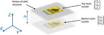
Figure 1. Portion of shell structure with strain sensors for input definition and global reference system [55]. Reprinted from [55], © 2022 Elsevier Ltd. All rights reserved.
Download figure:
Standard image High-resolution imageBeing only surface measurements available in most practical applications, the transverse shear strain  in equation (4) cannot be directly computed: it is neglected and set to zero given its contribution is negligible in thin shell structures.
However, in practical applications, sensors cannot be applied on the whole structure due to several constraints, such as restricted space, hardware limitations, and prohibitive cost. Thus, to mitigate this issue and increase the shape sensing accuracy, the measured strains can be interpolated or extrapolated on the whole domain before being fed as input to the iFEM. Among the interpolation/extrapolation techniques that have been applied in the literature [48, 49], the SEA is by far the most popular one. The SEA is a model-based algorithm that interpolate any continuous scalar field (i.e. any the strain component in the present case study) in a bidimensional domain. Its formulation is based on the minimization of a least-square penalty-constrained functional, similarly to what occurs in the iFEM. The interested reader can refer to its complete formulation in [50–52]. In brief, the structure is discretized with a shell triangular mesh where the dof are representative of the interpolated strain field. The functional of each element takes the form of equation (3), where the coefficients  and
and  should be properly set for each particular case study to obtain a smooth interpolating function, as described in [48],
Assembling the contribution of each element, the minimization of the SEA global functional is reduced to a linear problem, whose solution is the continuous field on the whole spatial domain. This solution is then used to feed the iFEM reasonable values of  and
and  in the elements where no direct experimental measurement is available.
Among the different inverse finite elements available in the literature, the specific element utilized in this work is the iQS4 element [46], whose formulation accounts for the shape functions developed for the MIN4 element [59, 60]. It is defined in local coordinates with a reference system origin in the centroid of the element, as shown in figure 2. Each node has 6 dof (3 translations and 3 rotations in the local reference system), thus each element has a total of 24 dof collected in the vector  , as reported in figure 2.
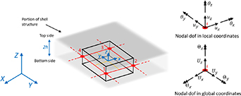
Figure 2. iQS4 element with local (lowercase letters) and global (uppercase letters) reference systems and degrees of freedom [55]. Reprinted from [55], © 2022 Elsevier Ltd. All rights reserved.
Download figure:
Standard image High-resolution imageThe dof  are linked to the numerical strain components as in the following equation:
where  ,
,  , and
, and  are matrices containing the derivative of the MIN4 shape functions [59, 60], which are not reported for the sake of brevity.
Finally, substituting equations (2) and (4) into equation (1), applying a standard assembly procedure to account for all the elements in global coordinates and minimizing the error functional with respect to the global dof (i.e.  ), the unknown displacements are the solution of the following linear problem:

It should be noted that the matrix  must be inverted only once in practice: the right-side term
  can be directly computed from the strain measurements, thus the nodal displacements of the structure are available in real time. Given the nodal displacements, it is straightforward to derive the strain field by applying equation (4).
2.2. iFEM extension for damage diagnosis
One fundamental assumption in the iFEM approach is the development of a model which is as representative as possible of the structure under analysis. Whenever a damage arises on the structure, the model may not be representative anymore of the real structure, and in that case the iFEM model computes an incorrect displacement field. This concept has been exploited to perform damage detection and diagnosis with the iFEM based on two approaches that are available in the literature:
- a DI approach, mainly devoted to damage detection, which is detailed in section 2.2.1.
- a model updating approach to perform damage quantification, which is detailed in section 2.2.2.
Both approaches make use of two sensor networks to perform damage diagnosis:
- an input sensor network (
 ), whose measurements are fed to the iFEM to reconstruct the displacement (and thus the strain) field on the whole domain.
 - a test sensor network (), whose strains are compared to the iFEM-reconstructed strains, to address the damage diagnosis task.


The two sensor networks may share sensors [53] or, to better highlight the presence of damage, have no sensors in common [57, 58].
The remainder of this is section is organized as follows: section 2.2.1 describes the DI approach and the extension to damage quantification that has been developed for this application, while section 2.2.2 outlines the model updating approach.
2.2.1. DI approach.
The DI approach, also called anomaly index in the iFEM literature, was originally introduced in [53] and it is hereby briefly described. As shown in figure 3, the input sensor network is initially employed to reconstruct the full field displacement and strain ( ) fields, which is then exploited to build a load-independent damage index
  for each test sensor location
  and for each time instant
  as:
as:

Figure 3. Damage Index (DI) framework with iFEM.
Download figure:
Standard image High-resolution imageIt should be noted that the original formulation [53] is based on the von Mises strain, while in the specific application of this work is simplified to the monoaxial strain components measured by fiber optic sensors.
The DI is a dimensionless metric of the difference between the reconstructed (iFEM) and the test strain field. The closer the index is to zero, the more the strain reconstruction at the test point is compatible with the real strain field ongoing on the structure, which is an indication of a healthy structure. On the contrary, a significantly high value of the DI suggests a mismatch between the iFEM-reconstructed strain and the measured strain, which points to the presence of damage on the real component.
The main weakness of this approach is that it is only built to perform damage detection; damage quantification has been performed in this work by identifying the test sensor with the highest DI.
2.2.2. Model updating approach.
A second damage diagnosis approach with iFEM has been recently introduced by Oboe et al in [57, 58] further exploiting the concept of compatibility between the real structure and its iFEM model. The key idea is to introduce the damage in the iFEM model to restore the compatibility between the model and the physical, damaged, structure. The compatibility, which in general is guaranteed only in the original undamaged condition, is restored with a maximum-likelihood model selection approach that determines the damaged condition that better matches the experimental measurements: the procedure is outlined as follows.
Several damage scenarios are generated off-line according to the expected damage mechanisms and stored in a database, although they might be generated in near real time according to the detected damage propagation, as demonstrated in [57, 58]. Afterwards, for each measured sample, the iFEM full field displacement and strain field are computed through the input sensor network for all the models, being the iFEM computationally inexpensive for real-time applications. Among all the models selected a-priori, the iFEM model that better matches the experimental evidence is selected through a MLE comparing the reconstructed strain field  with the test sensors
  . A zero-mean Gaussian likelihood is assumed for the error between the iFEM-reconstructed strain and each measurement in the test sensor network, so that the log-likelihood of the i-th model, considering all the measurements to be independent and identically distributed, is computed as:
where  is the number of test sensors considered and
  a variance parameter related to the measurement noise and the discrepancy between the model and the measurements. Finally, the problem is addressed with a MLE framework, where the model associated with the highest likelihood is selected as the most representative damage condition, as summarized in figure 4.

Figure 4. Model updating framework with iFEM.
Download figure:
Standard image High-resolution imageIt should be noted that maximizing equation (7) is equivalent to minimizing the squared error between reconstructed strain field  and the test sensors
  , thus the result is independent of the parameter
  . Nevertheless, the authors believe that framing the model selection through a likelihood function is still valuable since the problem may be readily extended to a Bayesian formulation to provide a maximum a posteriori estimate or to fully quantify the probability of each model according to the measurements, providing a more informative damage quantification. In case a Bayesian estimation is performed, the covariance matrix linking the measurements and the model may not take into account only the measurement as the error source and consider also the model error covariance. The model error covariance may be inferred from the measurements, or selected according to the domain expertise of the practitioner, considering both the measurement noise and the discrepancy between the model and the real structure, which may be estimated from a validation of the iFEM model in the undamaged condition, as outlined in [61]. For the sake of completeness, it should be noted that the assumption of independent measurements in the observational model may be questionable whenever the sensors are closely spaced: in this scenario the likelihood function should properly account for the spatial autocorrelation between the measurements.
It is worth noting that, since each iFEM model contains a different damage condition, the strain pre-extrapolation must be modified accordingly to properly account for the damage condition.
In conclusion, this approach aims to detect the most likely damage condition among a set of damaged scenarios selected a-priori considering any prior knowledge on the loading conditions and the expected damage mechanism, performing the damage parameters identification (e.g. size and location). However, it is worth mentioning that by knowing the material properties the iFEM might be employed to track the loading conditions, which may then be beneficial in updating the population of damaged scenarios and may be used in suitable damage propagation models based on direct FEM simulations, accomplishing prognostic tasks.
3. Case study
The two iFEM damage diagnosis approaches are applied on specimens representative of a bonded repair patch aiming to detect the debonding length, which is an application scenario where the iFEM has never been applied before in the literature This section is organized as follows: the specimens and the sensor network are presented in section 3.1, the experimental test rig is described in section 3.2, the debonding observations are presented in section 3.3; the iFEM models are outlined in section 3.4.
3.1. Specimens and sensor network
The tests have been carried out on two large CLS specimens with overall dimensions  , as depicted in figure 5. They are made of two carbon fiber reinforced laminates bonded by a film adhesive, mimicking a bonded repair patch on a damaged substrate. Since the goal of the experiment is to track the debonding front, a Upilex® film with a zigzag profile is inserted between the two laminates to initiate the debonding. The thickness of the specimens after manufacturing is
  in the single laminate region and
  in the double laminate one. Four steel tabs with a thickness of
  are bonded on each specimen with the 3M® DP490 epoxy adhesive to join the specimens to the testing machine.
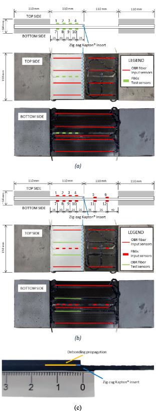
Figure 5. Specimen with steel tabs and strain sensors: (a) sensor network 1, (b) sensor network 2, (c) lateral zoom-in of the specimen. Input sensors are highlighted in red, test sensors in green. FBGs are represented by rectangles, OBR measurements by continuous lines. FBGs location are also represented in the lateral view of the specimen. All the sensors measure longitudinal strains.
Download figure:
Standard image High-resolution imageThe specimens have been equipped with two types of fiber optic strain sensors:
- A 3 m long optical backscatter reflectometry (OBR) fiber, which provides an almost continuous strain measurement along the whole fiber length.
- 12 fiber Bragg grating (FBG) sensors with a grating length of .

The sensors are installed on the specimen covering at best the external surfaces in a symmetrical pattern between the top and bottom sides. More specifically, the sensors measure only the strain component along the load direction and perpendicular to the expected debonding front, being the most informative in the present application. Sensor installation for an accurate acquisition of the transverse and shear strain components may be performed in practical application scenarios.
The available sensors are grouped into input and test sensor networks, as previously described in section 2.2. Moreover, to compare the performances of the DI and the model updating approaches as fairly as possible, each approach employs its own input and test sensor networks, which have been selected and are considered optimal by domain expertise:
- Sensor network 1 (figure 5(a)) is adopted for the DI approach (section 2.2.1). The input strain field is provided by the OBR fiber, while the DI is computed in correspondence with eight FBGs on the debonding propagation area.
- Sensor network 2 (figure 5(b)) is adopted for the model updating approach (section 2.2.2). The input sensor network is composed of some segments of OBR fiber and the 12 FBGs, while the test sensors are based on other OBR segments in the damaged area.
Two specimens share the same nominal sensor network and input-test definition, although some minor differences may be present due to the limited achievable precision in the OBR fiber placement. It should be noted that in a more realistic application scenario the location and the number of sensors may be optimized to detect the desired minimum detectable damage size by considering any prior knowledge on the expected loading conditions, boundary conditions and on the basis of engineering judgment.
3.2. Test rig
The specimens have been tested on a monoaxial MTS testing machine with a load capacity of  . A tension-tension fatigue load with
  and load ratio
  has been applied to propagate the debonding in between the two laminates. The load magnitude was tuned to achieve a stable debonding propagation and to limit the duration of the test. Strains have been acquired at discrete intervals (every
  cycles at the beginning of the test and every
  cycles during the stable propagation) at the static load of
  to avoid signal post processing issues on the optical fiber sensors. The OBR optical fiber has been acquired with a LUNA ODISI-B interrogator, providing quasi-continuous strain measurements with a gauge length of
  , while the FBGs have been acquired with a HBM DI410 interrogator. In addition to strain measurements, the debonding length at the two sides of the specimen has been directly observed through two Dino-Lite cameras on the two sides of the specimens, as shown in figure 6. A lateral view of the specimen with zoom-ins on the debonded interface is reported in figure 7, so that the debonding propagation can be fully appreciated. The total number of fatigue cycles performed and the number of data acquisitions are reported in table 1.

Figure 6. Test rig with an example image from a Dino-Lite camera. The lateral side of the specimen is painted in white to enhance the visibility of the debonding propagation by the camera observations.
Download figure:
Standard image High-resolution image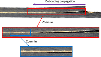
Figure 7. Specimen lateral view with zoom-ins on the debonded interface.
Download figure:
Standard image High-resolution imageTable 1. Number of fatigue cycles and data acquisition (strain and debonding length) for each specimen.
| Specimen N. | Fatigue cycles | N. acquisitions |
|---|---|---|
| #1 | 1450 000 | 70 |
| #2 | 1510 000 | 74 |
3.3. Debonding observations
During the experimental tests the strains and the real debonding length are measured at discrete intervals, as introduced in section 3.2. The debonding front at the two sides of the specimen observed through cameras is reported in figure 8 as a function of the number of cycles. The damage extension is not symmetric between the two sides of the large CLS. Both specimens exhibit the same behavior, with the right side propagating faster than the left one: this behavior, according to the author's domain expertise, is most likely induced by a misalignment of the testing machine that introduces an undesired torsional contribution. For the sake of clarity, it is remarked that in a real SHM system these observations are not available (if not by means of visual inspection), and thus they are the target to be inferred from the strain measurements.

Figure 8. Real debonding length observed through the two cameras on the Large CLS specimens as a function of the number of fatigue cycles: (a) specimen #1, (b) specimen #2.
Download figure:
Standard image High-resolution image3.4. iFEM model
The iFEM model developed for the large CLS specimen is described in this section. The model in the undamaged configuration is reported in section 3.4.1 and the SEA strain pre-extrapolation model in section 3.4.2. Section 3.4.3 presents how the model is systematically modified to account for different damage conditions and how a database of damaged scenarios is built.
3.4.1. Undamaged iFEM model.
The iFEM model of the specimen is representative of its effective useful length, i.e. excluding the tabs required to connect the specimen to the testing machine. Thus, the model has a total length of  and a width of
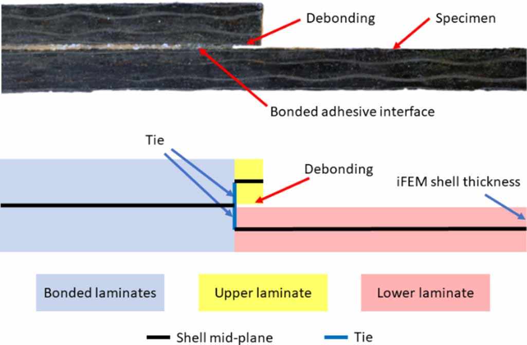
  . The inverse shell elements are defined in the mid-plane of the shell, thus three different shells are employed to model the specimen, as represented in figures 9 and 10:
- A single shell having a thickness of represents the region in which the two laminates are bonded by the film adhesive (bonded laminates),
- A shell of thickness for the single laminate region (lower laminate),
- A shell of thickness for the bonded laminate in the debonded region (upper laminate).


Figure 9. iFEM model in the undamaged condition (debonding length of  ).
).
Download figure:
Standard image High-resolution image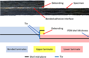
Figure 10. Side view of the iFEM model with tie definition.
Download figure:
Standard image High-resolution imageThe three shells are not physically connected with each other since they are defined on different planes, thus tie constraints are inserted to restore the continuity of the dofs, as shown in figure 10. It should be noticed that, although this model refers to the undamaged condition of the specimen, an initial debonding of  has been modeled to reproduce the effect of the zigzag Upilex® insert.
The applied boundary conditions are representative of the steel tabs and the test rig, with one side of the specimen clamped and the other side in which only the longitudinal displacement is allowed, as highlighted in figure 9. Finally, the structure is discretized into  iQS4 inverse shell elements.
3.4.2. SEA model.
Before feeding the measured strains to the iFEM, the strain field acquired from sensors is pre-extrapolated on the whole domain with the SEA. The SEA model shares the geometry with the iFEM model; however, the SEA mesh, which is not reported for brevity, is coarser than the iFEM one, and it composed of  triangular elements.
The strain field on the top and bottom sides of the specimen are pre-extrapolated independently, as it is common practice in the pre-extrapolation literature. However, the two extrapolations are based on slightly different models due to the geometrical complexities previously discussed. When pre-extrapolating the top side of the specimen, two separate external surfaces can be intuitively identified, namely surface 1 and surface 2, highlighted in red in figure 11. Being the two surfaces subjected to a different strain field, the two portions of the SEA model are unlinked and thus pre-extrapolated independently. Surface 1 contains two model surfaces: the upper surface of the so-called bonded laminates region and the surface of the so-called upper laminate region, the latter being representative of the debonded patch. Thus, these two surfaces are linked together through a tie constraint to restore the continuity of the dof, as shown in figure 11.
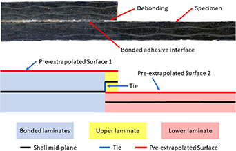
Figure 11. SEA schematic model to pre-extrapolate the strain field on the top side of the specimen.
Download figure:
Standard image High-resolution imageA similar framework defines the SEA model to pre-extrapolate the strain field on the bottom side of the specimen, as reported in figure 12. In this case, the bottom side of the specimen is composed of one single surface, namely surface 3, which is the union, through a tie constraint, of the bonded laminates lower surface and the lower laminate lower surface. The bottom side of the upper laminate region represents an additional surface to be pre-extrapolated. It should be noted that this surface is not interested by any sensor since it is representative of the debonded interface. However, once the upper laminate debonds from the substrate, this surface becomes a stress-free region and thus the strain of this region is set equal to zero.

Figure 12. SEA schematic model to pre-extrapolate the strain field on the bottom side of the specimen.
Download figure:
Standard image High-resolution imageFinally, since sensors measure only the strain component along the longitudinal ( ) direction, the other strain components (i.e.
  and
and  ) are not pre-extrapolated and set equal to zero on the whole structure. Thus, only the longitudinal strain component is investigated in this case study.
3.4.3. Database of damage models.
Once the iFEM model and the respective SEA models have been defined in the undamaged condition, different debonding conditions are considered to create a database of damage scenarios.
The debonding front is assumed to be perpendicular to the longitudinal direction of the specimen, thus the debonding front can by parametrized by a  , which is increased from the undamaged condition (
 ) up to
  with a step increment of
  , generating a total of
  models. It is worth remarking that, as mentioned in section 2.2.2, although in this paper the models are generated a-priori for the sake of simplicity, they might be generated online in near real time according to the detected damage propagation and the estimated loading conditions, e.g. the case in which one side of the joint is debonded and the other is intact may be modeled. It should also be noted that the assumption of the debonding front being straight and perpendicular to the longitudinal direction may not utterly reflect the experimental evidence; nevertheless the assumption is deemed a reasonable trade-off between model complexity and data fit for the case study at hand. More specifically, this assumption is necessary to maintain a structured iFEM mesh with perfectly rectangular elements since the experimental strain measurements are only available along the
  direction of the specimen. In fact, the creation of a distorted mesh (with non-rectangular elements) requires additional transformations from the global to the local reference system, inducing numerical errors in case all the plane strain components (i.e.
  ,
,  , and
, and  ) are not acquired, as thoroughly illustrated in [44].
The iFEM model generated for a debonding length of  is reported in figure 13 as a representative example. It should be noted that, for each iFEM model considered, also the two corresponding SEA models for strain pre-extrapolation are generated.
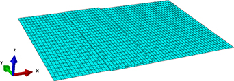
Figure 13. iFEM model with a debonding length of  .
.
Download figure:
Standard image High-resolution image4. Results and discussion
In this section the iFEM results obtained for the two specimens are presented and discussed: section 4.1 outlines the shape-sensing results obtained with the iFEM, while in sections 4.2 and 4.3 the performances of the two diagnostic approaches are evaluated.
4.1. Shape sensing: undamaged scenario
The iFEM algorithm is applied to reconstruct the displacement and strain fields of the specimens under analysis. For the sake of brevity, this section presents only the shape sensing results obtained on specimen #1 with sensor network 2, although comparable results are obtained also with the other specimen and sensor network. The displacement and strain fields reported in this section are computed with measurements taken from the undamaged structure, thus the undamaged iFEM model is adopted (i.e. considering a  debonding length).
Although the combination of SEA and iFEM is already outlined in section 2.1, the passages are hereby reported for the sake of clarity. The strain measurements from the input sensor network are associated to the respective iFEM elements, as shown in figure 14. These measurements are fed to the two SEA models so that the strain field is pre-extrapolated on the whole domain and then fed to iFEM, as shown in figure 15. As described in section 3.4.2, the pre-extrapolated strain field follows the input measurements in the upper side of the laminate and the bottom side of the upper laminate is set to zero in the debonded region. Furthermore, since only the strain component  is acquired form sensors, the components
  and
and  are arbitrarily set equal to zero. This strain field is fed to the iFEM routine to compute the nodal displacements of the mesh. The displacement field is rendered in figure 16: the elongation along the longitudinal direction is almost symmetric, with a maximum amplitude of
  , while the out-of-plane displacement is not symmetric. Specimen #2 presented very similar asymmetric displacement, which, as discussed in section 3.3, is most likely due to a torsion load induced by a misalignment of the testing machine. Finally, the iFEM-reconstructed strain field is computed from the displacements through equation (4) and the results are depicted in figure 17. Although this strain field is qualitatively similar to the pre-extrapolated strains (figure 15), the iFEM-reconstructed strains are the results of the iFEM minimization process and not just of a pre-extrapolation (interpolation) algorithm. More specifically, the iFEM guarantees the compatibility of displacements and accounts for the boundary conditions, while the pre-extrapolation is carried out independently for each strain component and without guaranteeing any compatibility among them.
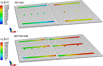
Figure 14. Input strain field ( ) acquired by sensors for specimen #1 in the undamaged configuration.
Download figure:
Standard image High-resolution image
Figure 15. Pre-extrapolated input strain field for specimen #1 in the undamaged configuration.
Download figure:
Standard image High-resolution image
Figure 16. Shape sensing results (displacement field  ) for specimen #1 in the undamaged configuration. Deformed shape with a scale factor of 50.
Download figure:
Standard image High-resolution image
Figure 17. Numerical strain field computed by the iFEM ( ) for specimen #1 in the undamaged configuration. Deformed shape with a scale factor of 50.
Download figure:
Standard image High-resolution image4.2. DI approach
This section presents the performances of the DI approach for damage identification. The strains measured by the sensor network 1 are fed to the iFEM routine with the undamaged model ( mm debonding). Once the numerical strains (
 ) are computed, the load-independent DI introduced in section 2.2.1 is computed in correspondence of the eight test sensors. For each test sensor, the DI is displayed as a function of the number of cycles, as reported in figures 18 and 19 for specimens #1 and #2 respectively. The first acquisition frame is performed with the structure in its original condition, without any significant debonding propagation. For this reason, although a small DI is computed due to measurement noise and other experimental uncertainties, this is considered the initial reference condition and thus this is taken as a baseline and any bias is removed.

Figure 18. Damage index as a function of the number of fatigue cycles for specimen #1. Only three vertical dashed lines are plotted since the test was stopped before the debonding front reached FBGs 1 and 7.
Download figure:
Standard image High-resolution image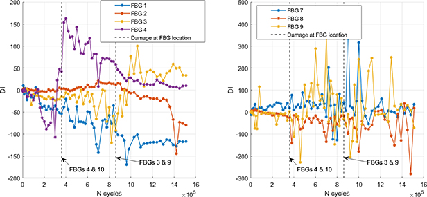
Figure 19. Damage index as a function of the number of fatigue cycles for specimen #2. Only two vertical dashed lines are plotted since the test was stopped before the debonding front reached FBGs 1, 2, 7 and 8. FBG 10 was not plotted since the interrogator was unable to connect to it.
Download figure:
Standard image High-resolution imageThe debonding front location can be inferred from the DIs since, as soon as the debonding propagates inside the specimen, the  increases in magnitude highlighting the presence of the damage since the iFEM strains are computed with the original iFEM model in the undamaged condition. More specifically, a trend in the DIs is observed: the DI increases sharply whenever the debonding front propagates underneath the sensor; the DIs of FBGs 4 and 10 are the first to manifest a significant trend since these sensors are the closest to the debonding front propagation starting point. To make it clearer, vertical dashed lines are plotted in figures 18 and 19: they represent the number of cycles associated with an average debonding length (averaged between the observations of the left and the right camera) in correspondence of the FBGs locations; in other words, they highlight the time instant at which the debonding front propagates underneath the sensor location. It should be noted that this time instant is just a reference value, since the real debonding front shape may not be linear between the left and right sides of the specimen.
Whenever the debonding front propagates underneath the FBGs, the  (of FBGs 4 and 10) assumes its highest value (in magnitude) and a change of trend is observed. In addition, it should be noted that the
  of FBG 4 is initially negative and then becomes positive, while FBG 10 exhibits the opposite trend. This behavior is associated with an incorrect computation of the iFEM curvature field since the input strain is affected by damage while the iFEM model considered has been defined in the healthy condition. The same
  trend can be observed for FBGs 3 and 9 as soon as the average debonding length reaches a length of
  and for FBGs 2 and 8 with a
  debonding length.
As shown in figures 18 and 19, the results obtained for specimens #1 and #2 are very similar to each other, confirming the reproducibility of the experiments. Only the damage indices computed on the bottom side of specimen #2 (i.e. FBGs #7 to #10 in figure 19) are affected by a high level of noise and uncertainties due to technical issues encountered during the experimental test.
In conclusion, the DI approach applied to the case study under analysis can detect the presence of the damage and it could be used to preliminary estimate its size by interpreting the DI trends as a function of the test sensor locations. However, since the DI are not a physical quantity, selecting a threshold on the DIs trends to perform damage quantification is not straightforward and this approach should be tailored for each specific application: thus, a more accurate damage quantification can be performed with the model updating approach presented in the next section.
4.3. Model updating approach
This section presents the performances of the damage size estimation by model updating. Strains are taken from sensor network 2 and they are processed as described in section 2.2.2: the input strains acquired at each time instant are fed to all the iFEM models in the healthy and in the damaged conditions, and the respective displacement and strain fields are computed. Then, the  computed by each model is compared to the test measurements through the likelihood function, obtaining an indication of the agreement of every single model with the real, damaged, structure. Although the value of
  does not affect the MLE, as mentioned in section 2.2.2, for the sake of completeness
  is used in this study, which is considered representative of the measurement noise and of the discrepancy between the measurements and the model.
The log Likelihood obtained for the strain acquisition performed after  fatigue cycles on specimen #1 is reported in figure 20 as a representative example: the debonding length MLE is
  , which lies in between the two debonding observations performed through the cameras, thus identifying an intermediate damage condition. The likelihood function sharply decreases from the MLE value highlighting a lower agreement between the iFEM model adopted and the real structure: to appreciate a qualitative correlation between the likelihood behavior and the iFEM results, the strain field of three iFEM models are also reported in the figure. The
  model, which better identifies the damage condition, computes a displacement and strain field that fits the condition of the structure, taking also into account the results obtained for the undamaged case (section 4.1). On the contrary, the
  and the
  models are associated with an odd reconstruction of the curvature due to the erroneous damage imposed by the models. Accordingly, the strain fields manifest significantly different ranges (with respect to the
  model) and they show steep strain gradients near the boundary conditions.
Figure 20. Likelihood trend for the strain acquisition after 700 000 fatigue cycles on specimen #1. iFEM strain results on the top side of the specimen for different models and deformed shapes with a scale factor of 50.
Download figure:
Standard image High-resolution imageTo picture the performances of the model updating approach, the MLE of the debonding length at each acquisition is reported in figure 21 in comparison with the debonding measured by the two cameras. The MLE is generally in between the debonding length measured on the two sides of the specimen, highlighting that the modeling assumption of the debonding front being perpendicular to the longitudinal direction of the specimen does not affect the model selection, and the MLE is consistent with the experimental observations.

Figure 21. Debonding length detected with the model updating approach: (a) Specimen #1, (b) Specimen #2.
Download figure:
Standard image High-resolution imageDiscrepancies are mainly condensed at the beginning of the fatigue life, where the MLE of damage is significantly different from the measured values from the camera: this, in the authors' opinion, is due to the low sensitivity of the sensor network to minor debonding sizes. More specifically, debonding lengths up to about  do not induce significant strain variations on the input sensors since the first OBR sensors on the top side of the specimen are located at about
  from the free end of the upper laminate. This can also be inferred from the likelihood trend at
  fatigue cycles on specimen #1, which is shown in figure 22 as a representative example. The Likelihood function up to about
  of iFEM debonding length is almost flat, highlighting little advantage (in terms of MLE or minimum RMSE) in selecting one or another damaged condition. It should be noted that this issue may be bypassed with a more accurate design of the sensor network with respect to the minimum detectable damage size required by the SHM system. In addition, although a MLE (which is equivalent to the minimum RMSE) of the damage is found, under these circumstances it is a fragile estimator since it does not provide any information on its robustness and about whether the modeling assumptions (i.e. the sensors are affected by the debonding) actually hold. Even though it is left for future research, a Bayesian approach should be favored in this context, possibly considering the model error source in the observational model, as described in section 2.2.2. In light of these considerations, the MLE of the debonding length provides valuable information on the agreement between the iFEM models and the real structure whenever the sensors are non-negligibly affected by the debonding, and it is deemed a reasonable choice to identify the model that better describes the real damage.

Figure 22. Likelihood trend for the strain acquisition after 40 000 fatigue cycles on specimen #1.
Download figure:
Standard image High-resolution image
In conclusion, the model updating approach presented can successfully identify the iFEM model that better represents the actual damaged condition of the structure, with a good agreement with the experimental observations, although only iFEM models with straight debonding fronts are generated. In a more realistic application scenarios, more complex damage models may be implemented.
5. Conclusions
This paper applies for the first time the iFEM to specimens' representative of adhesive bonded joints and repair patches, proposing two approaches to quantify the debonding.
The first approach is an extension of the state of the art in the iFEM damage detection algorithms: it correlates the debonding entity to a trend in the anomaly indexes of the sensors, which are based on the discrepancy between the measured strains and the iFEM-reconstructed strain through a healthy model of the structure. The DIs sharply increase whenever the debonding front propagates underneath the sensors; however, the performances of this methodology for damage quantification is limited by the fact that the interpretation of such trends in the DIs signals is not straightforward, and this approach may have to be tailored for each specific application.
The second approach proposed in this paper, which is applied for the first time on adhesive-bonded patches, is based on a maximum likelihood estimation of damage: several iFEM models with different debonding entities are generated and compared through a likelihood function: the model whose iFEM-reconstructed strains are most in agreement with the data is selected, providing an estimate for the debonding entity. This approach has demonstrated satisfactory performances on CLS specimens representative of composite repair patches, thus it is deemed a significant research step with respect to the current state of the art.
The main drawback of the proposed approach is the number of required sensors and their positions, which should be placed either on both sides of the specimen or embedded in two plies of the composite material, so that the shell curvature and membrane strains can be computed.
Future iFEM research in the context of adhesive bonded connections may be devoted to modeling more complex debonding shapes, since the present work considers only straight debonding shapes, to optimizing the sensor network to lessen the number of sensors, and to validate the methodology on more complex case studies, including repair patches applied on real aircrafts. The methodology itself may be improved by applying Bayesian inference techniques to quantity the uncertainty of each model, thus quantifying the debonding front probability mass function, and by coupling the model updating approach with prognostic tools such as Bayesian filters to track the degradation process, estimating the residual useful life of the monitored component in real time.
Acknowledgments
This work has been developed based on the results from PATCHBOND II (Certification of adhesive bonded repairs for Primary Aerospace composite structures), a Cat.-B project (No B.PRJ.RT.670) coordinated by the European Defense Agency (EDA) and financed by the following nations: The Netherlands, Norway, Italy, Germany, Finland and Czech Republic.
Data availability statement
The data cannot be made publicly available upon publication due to legal restrictions preventing unrestricted public distribution. The data that support the findings of this study are available upon reasonable request from the authors.