


Abstract
Robustness to noise and independence from a prior state are phenomena often believed to be determined by the overall topology of a network. We show that these features can instead be present at the level of a single limit cycle, representing the activity of a small group of neurons inside a cortical column. In particular, we find a bifurcation where this limit cycle changes from being susceptible to noise to being remarkably robust to noise, such that any history of input is erased over a single oscillation. We then show how this property leads to spatially patterned synchronization and pattern expression when many such limit cycles are coupled in a large-scale model of the superficial layers of the visual cortex.
Export citation and abstract BibTeX RIS

Content from this work may be used under the terms of the Creative Commons Attribution-NonCommercial-ShareAlike 3.0 licence. Any further distribution of this work must maintain attribution to the author(s) and the title of the work, journal citation and DOI.
1. Introduction
The relationship between network topology and network dynamics has been an active area of research in recent years [1–6]. Of special interest are network topologies which show properties common to cortical networks, such as robustness to noise and variation [7–9] and the ability to display various synchronization modes [10–12]. Although local synchronization has been extensively investigated in neural networks, recent experimental [13] and theoretical [14] works suggest that it may play a smaller role in cortical processing than has been thought. This implies greater importance of long-range spatially patterned synchronization, which has been suggested as a mechanism for feature binding and therefore pattern recognition in the mammalian visual cortex [15, 16]. It is of particular importance to understand how this long-range synchronization arises in networks with comparable numbers of local and long-range periodic excitatory coupling, reflecting the coupling architecture of mammalian cortex [17–19].
The robustness of a network to noise, or its sensitivity to random perturbations, has been extensively studied. Although some recent works have indicated that intrinsic properties of individual network components can provide robustness to network dynamics [20, 21], the noise robustness feature is often believed to be determined by network topology. For instance, chaotic dynamics (which show enhanced sensitivity to perturbations) have been attributed to sparsely but strongly connected large networks of excitatory and inhibitory neurons [22], while stable, although seemingly irregular, dynamics have been attributed to networks with delayed inhibitory interactions [4, 5]. Noise robustness was also found to differ substantially between feedforward and attractor networks, with feedforward linear networks having increased robustness due to the removal of noise when the signal exits the network [23]. Other recent investigations have focused on the reconstruction of network topology given its response to different driving conditions [1], indicating that there is a one-to-one correlation between the noise response and the coupling architecture of the network [2].
In this paper, we show that in certain cases the noise robustness of a network and independence of prior history can be inferred from the investigation of a single limit-cycle oscillator, independent of the overall topology. We then show using biologically realistic parameters how this property leads to long-range spatially patterned synchronization in a cortical column model with comparable numbers of local and long-range connections. In particular, we find that the network is robust to noise during the majority of an oscillation cycle, but has a 'reset' point whereby a new pattern can be chosen independent of previous activity. We employ contraction analysis [24] to show that the relative strength of local and spatially periodic long-range coupling shapes spatial patterns of synchronization. Our results suggest that while connection topology is crucial in determining the synchronization patterns of a network, the properties of individual oscillators can confer robustness to noise and independence of history that is characteristic of the primary processing areas of the cortex.
The cortical network presented here may be particularly suitable for the reconstruction of its topology based on the method of compressive sensing. Using this method, the network topology can be recovered from a limited number of measurements [25, 26]. While the robustness of this reconstruction has been tested on a time series contaminated by noise and shown to be reasonably robust [27], the minimum number of measurements required for accurate reconstruction is expected to increase with noise. The robustness of the network presented here ensures that a recorded time-series would reflect topology-dependent neural correlations, largely uncorrupted by noise, therefore necessitating sparser data requirements for accurate reconstruction.
2. Elemental oscillator unit: dynamics and stability
Our elemental unit is a Wilson–Cowan oscillator consisting of a recurrently coupled pair of excitatory and inhibitory linear-threshold neurons (see figure 1), each representing a small population of neurons in a cortical column [28]. A linear-threshold neuron model is a reasonable approximation to the current-to-firing-rate (IF) transfer function of adapted cortical neurons [29]. The network is described by

where xj and yj represent the internal activation of the excitatory and inhibitory members of the elemental unit j; τE and τI are the time constants of excitation and inhibition; α and β are the strengths of recurrent excitation and inhibition; ![$\left [z\right ]^{+}$](https://content.cld.iop.org/journals/1367-2630/14/12/123031/revision1/nj445313ieqn1.gif) denotes the linear-threshold function
denotes the linear-threshold function ![$\left [z\right ]^{+}=\max \left (z,0\right )$](https://content.cld.iop.org/journals/1367-2630/14/12/123031/revision1/nj445313ieqn2.gif) ; Ij is the input current injected into unit j; and
; Ij is the input current injected into unit j; and  is a Wiener process that is independent for each neuron, and has standard deviation σ after 1 s. All parameters are positive and real.
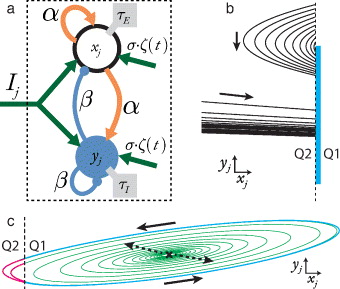
Figure 1. (a) The basic columnar unit analysed in this paper and described in equation (1). (b) Trajectories of a single element pass from quadrant 2 (Q2) into quadrant 1 (Q1) within a restricted range of values for yj (marked region). (c) When an elemental unit is driven with an injected current Ij, it produces limit-cycle oscillations under certain parameter constraints. The dynamics are characterized by an unstable spiral fixed point in Q1 (black cross, dashed arrows); asymptotic decay in Q2; and a limit-cycle trajectory that passes through Q1 and Q2 (outermost trajectory). Dashed lines: boundary between Q1 and Q2.
Download figure:
Standard imageWe define the state of the elemental unit in terms of the phase space defined by xj and yj. Quadrant 1 (Q1; xj, yj > 0) of the phase space exhibits the most complex dynamics and contains a stable or unstable spiral fixed point when

where  and
and  . Asymptotic stability in Q1 is guaranteed when α < β + 1 and the upper bound on τI in equation (2) is satisfied. In Q2 (xj < 0, yj > 0) the activity in the system dissipates towards a stable node fixed point located in Q1. States in Q3 (xj,yj < 0) and Q4 (xj > 0, yj < 0) always lead to a transition to Q2 or Q1, constraining the dynamics to remain in the upper half plane. It is easily seen that if the fixed point in Q1 is an unstable spiral, then the system must move into Q2 in finite time. Since crossing into Q2 bounds the system dynamics, it follows that all fixed points with complex eigenvalues will have bounded trajectories, resulting under the Poincaré–Bendixon theorem in either a globally stable fixed point or at least one stable limit cycle [30–32].
2.1. Limit-cycle trajectories
As has been shown previously, an elemental unit of this form can behave as a limit-cycle oscillator [28, 33, 34]. Two possible types of limit-cycle oscillations can occur, separated in parameter space by a Hopf bifurcation whereby the fixed point in Q1 changes from stable to unstable. In the first case, corresponding to a stable fixed point with complex eigenvalues, a limit cycle is possible if the dynamics are started outside of the basin of attraction of the fixed point. In this case, however, the trajectory is sensitive to noise which can push the limit cycle into the stable basin, whereby the oscillatory behavior is extinguished. As we show, the second case, where the fixed point in Q1 is unstable with complex eigenvalues (resulting in a globally stable limit cycle), exhibits independence of prior history, which is crucial for new pattern selection on each subsequent oscillation.
We show the robustness of this limit cycle to noise by deriving an upper bound on the greatest possible separation of any two trajectories transverse to the limit cycle over a single oscillation. This upper bound is obtained by examining the crossing of trajectories from Q2 into Q1 and showing that they are bounded from above and below. From equation (1), the dynamics of a trajectory in Q2 are given by  and
and  . Since
  for y < I/β, the trajectory will only cross from Q1 into Q2 if y > I/β. By the same argument, the trajectory crossing from Q2 into Q1, will have to satisfy y < I/β, providing the upper bound ymax = I/β. To derive the lower bound we observe that motion along the y-axis in Q2 is independent of x and asymptotically approaches the fixed point
  from above, so that
  while the trajectory is in Q2, therefore
  . Therefore the upper bound on the possible separation, Δ, of any two trajectories crossing from Q2 into Q1 is given by

This system therefore has an unusual property that regardless of the level of noise, the maximal transverse separation of any two trajectories at a certain phase of the oscillation is given by the above inequality. An interesting feature of the above bound is its independence of excitation, α, and rather sensitive dependence on inhibition, β. It is therefore possible to change the robustness to noise of the network while keeping the ratio of inhibition of excitation constant.
2.2. Application to the cortex
If we interpret the two neurons in the simple column model to correspond to pyramidal (excitatory) neurons and basket cell (inhibitory) neurons in the superficial layers of cat visual cortex, then we can use estimates of the synapse number and strength to derive approximate parameter values [19, 35]. The weighted connections (both local and long-range) arising from the excitatory neuron wE therefore sum to 2.71, with α = 2.71 for the single-column model. Likewise, the inhibitory connections wI sum to 5, with β = 5 for a single column. We can also define a relationship between the short- and long-range excitatory coupling strengths γS = wEλ and γL = wE(1 − λ), respectively, such that wE = γL + γS, where 0 ⩽ λ ⩽ 1. Time constants τE and τI correspond to lumped values reflecting the overall time course of spike-to-spike activation patterns in populations of neurons, including facilitation. A population of inhibitory neurons in rodent cortex has a considerably slower time course of activation than the excitatory population [36]. We used these data to estimate parameters for the time constants of excitation and inhibition at τE = 4 ms and τI = 35 ms.
We estimated the distribution of spontaneous input currents that impinge on single neurons of these classes by combining the synapse counts, the average pre-synaptic spontaneous rate [37] and the average post-synaptic charge delivered by a spike [35]. We simulated these values with Poisson spike trains and obtained parameter estimates for equation (1) of I ≈ 1 × 10⁻⁷ and σ ≈ 4 × 10⁻⁹ to 5 × 10⁻⁹.
For the parameter values given here, the maximum separation of trajectories crossing from Q2 into Q1 from equation (3) is Δmax ≈ 3 × 10⁻⁹. This corresponds to approximately 1% of the width of the limit cycle. This value is nearly constant for different values of the input current, since both the maximal width and the size of the limit cycle scale linearly with I.
While the separation between two trajectories will increase after crossing into Q1 due to both the instability of the fixed point in Q1 as well as the effects of noise, they will converge again after exiting Q2, within the narrow bound given by equation (3). In particular, any effect of noise will be erased over a single oscillation.
3. Synchronization of coupled oscillators
We study the possible synchronization patterns in a network of recurrently coupled neural oscillators using contraction theory [24]. The four-column network discussed here is an analytically tractable model of a large-scale ring network, described below. For this simple case, the recurrent couplings are illustrated in figure 2(a) and consist of short-range couplings (solid lines) and long-range couplings (dashed lines). The Jacobian of this system in Q1 is given by
where  is the 4 × 4 identity matrix. The system in figure 2(a) can exhibit two synchronization modes: one where the units coupled through γL are pair-wise synchronized (M×) and one where all four units are synchronized (M*). Exponential convergence to Mi, i = ×,*, is guaranteed if the subspace Mi is flow-invariant [38, their equation (5)]; if there exists a metric Θ such that ΘΘ⊤ is positive definite; and if
 ![$\lambda _{\max }\left [\Theta V_{i}JV_{i}^{\top }\Theta ^{\top }\right ]=m_{i}<0$](https://content.cld.iop.org/journals/1367-2630/14/12/123031/revision1/nj445313ieqn13.gif) , uniformly, where
, uniformly, where ![$\lambda _{\max }\left [X\right ]$](https://content.cld.iop.org/journals/1367-2630/14/12/123031/revision1/nj445313ieqn14.gif) is the maximum eigenvalue of the Hermitian part of X and Vi is the projection to the space spanning the null of Mi. V× and V* are given by
is the maximum eigenvalue of the Hermitian part of X and Vi is the projection to the space spanning the null of Mi. V× and V* are given by

If these conditions are satisfied and then the system is contracting, i.e. all the trajectories projected on Mi converge exponentially fast, with the contraction rate given by mi [24]. If Θ is a constant metric, then ΘΘ⊤ is always positive definite. The linearity of the dynamics in each quadrant allows us to choose Θ such that it diagonalizes ViJV⊤i [39]. In this case, mi is equal to the eigenvalue with the largest real part. For M* and M×, figure 2(b) shows the contraction rates mi in Q1 for the long-range coupling proportion λ varied between 0 and 1.
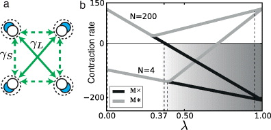
Figure 2. (a) Four recurrently coupled elemental units, with excitatory long-range  and short-range
  couplings. Recurrent connections are as in figure 1. (b) Contraction rates for M* and M× versus the long-range coupling proportion λ, for the cases of 4 and 200 oscillator elements. The discrepancy between the two cases is due to the different relationship in the extent of the short-range and long-range connections.
Download figure:
Standard imageIn Q1, the network can express spatial activity patterns, driven by spatially patterned synchronization, if m× < m* and m× < 0. These bounds are shown in figure 2(b) for networks with 4 and 200 oscillator elements (vertical dashed lines). The couplings in the latter case were the same as those shown in figure 3. If m* < 0, in addition to the bounds given above, then the globally synchronized state is also stable. This implies that the spatial activity patterns are expressed only transiently in Q1, because the uniform synchronization pattern is a special case of the spatial activity pattern (M*⊂M×).

Figure 3. (a) Large-scale ring model with short- and long-range coupling. (b), (c) Parameter regimes derived numerically from the large-scale system (shading) match those obtained analytically from a single-element system (dashed curves). The boundary between regions II and III depends on the topology of lateral coupling and cannot be derived from the single-element system. The parameters used in simulations are indicated by circles. Regions: I: asymptotic stability; II: asymptotic stability with a non-dominant complex eigenvalue; III: stable spiral fixed point; IV: unstable spiral fixed point; V: exponentially divergent unstable fixed point.
Download figure:
Standard imageIn Q2, the neural oscillators are independent of each other. Because each oscillator converges to a common fixed point, the network synchronizes globally, i.e. M* is always stable. Consequently, even when m* > 0 in Q1, or m× < 0 and m× < m*, the network may still fully synchronize. Nevertheless, since λ = 1 corresponds to a network of disjoint groups of oscillators, it is expected that the dynamics converge to M× when λ approaches 1. The precise boundary value cannot be computed analytically due to the nonlinear behavior of the oscillators, but it is observed in the simulations described below.
4. Large-scale systems and pattern expression
We implemented a linear ring model composed of 200 oscillator elements (see figure 3(a)). The local recurrent coupling of each element was as shown in figure 1(a). Uniform lateral excitatory coupling extended for five nearest neighbours up and down the ring; periodic long-range coupling was introduced between groups of neurons separated by 20 elements, resulting in 20 groups of 10 elements each. Every position around the ring had an identical pattern of connections.
The parameter bounds that define regions of stability and of oscillatory behaviour generalize remarkably well from the single-element oscillator to large-scale systems when the network connectivity is homogeneous (i.e. the connections from each element are identical across the network). The parameter regimes established by varying τE, τI, wE and wI in the large-scale ring model match the analytical boundaries derived from the single-element oscillator (figures 3(b) and (c)), and are therefore independent of the size of a model system. The basic dynamics of a large-scale model can therefore be known from the analysis of a single system element. Limit-cycle dynamics are possible only in regions III and IV, and are guaranteed only in region IV.
Noisy currents injected into the model caused limit-cycle oscillations, as for the single-element oscillator, when the network was in a favourable oscillatory regime. In this regime, the proportion of long-range excitatory coupling λ determined the form taken by spatial patterns of synchronization across the network (see figures 2(b) and 4). For the permissive values of λ described above, synchronization occurred preferentially between elements coupled through long-range connections, allowing the spatial arrangement of long-range coupling to be expressed in activity states of the network (figures 4(c) and (d)).
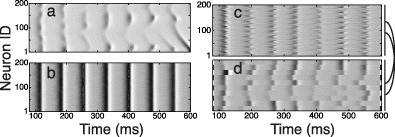
Figure 4. The large-scale ring network exhibited limit-cycle oscillations, with various spatial modes of synchronization. Synchronization occurred either locally ((a) λ = 0), globally ((b) λ = 0.37) or mediated via long-range connections ((c), (d) λ = 0.95). In this last case, synchronized oscillations resulted in the expression of spatial activity patterns. Panel (d) shows the same activity as (c), but with neurons grouped according to their long-range partners. A different spatial activity pattern is selected during each limit-cycle oscillation.
Download figure:
Standard imageThe effect of the noisy input currents on this system varies over the course of a single oscillation cycle. During the initial phase of an oscillation the amplitude of network activity is small with respect to injected noise, resulting in desynchronization of the network. Subsequently, groups of elements coupled through long-range connections of appropriate strength were able to synchronize, resulting in the expression of a randomly chosen spatial activity pattern (figures 4(c) and (d)). However, the amplitude of network activity grows rapidly due to fast recurrent excitation unchecked by the slow inhibitory activity (figure 1(c)), and the selected spatial pattern is therefore quite robust to perturbation by the constant-variance noise. The limit-cycle trajectory of the system provides a built-in reset of the network, returning network activity to a common state of low activity via slow and strong inhibition in Q2. As the network returns to relative quiescence, the amplitude of noise once again desynchronizes the network and allows a new activity pattern to be selected.
Importantly, the robustness to perturbation conferred by the intrinsic dynamics of single oscillators was not reduced by introducing the large-scale network topology. To test this, we examined the insensitivity to noise of the network under various combinations of short-range and long-range coupling (i.e. λ = 0, short-range coupling only; λ = 0.5, a balance between short- and long-range coupling; and λ = 1, long-range coupling only). Perturbations were added in the form of initial condition noise and brief pulses injected into portions of the network. While spatial synchronization patterns differed strongly for varying λ (see figure 4), the noise robustness of the network to perturbations was similar in all cases. In particular, for all relative strengths of long- and short-range excitatory coupling λ, the perturbation bound Δ in equation (3) was found to hold.
5. Discussion
In conclusion, we have shown that a limit cycle representing averaged neural activity can exist in two possible states, the intermediate and the strong stability regime (stability regions III and IV in figures 3(b) and (c)). Partial robustness to noise exists in the intermediate regime, but it is possible for external input to silence the oscillations. In the strong stability regime, the system is exceptionally robust to noise to the extent that all perturbations are reduced to within bounds derived above, over the course of a single oscillation. A reasonable choice for cortically realistic parameters places the oscillator in the strong perturbation-limiting regime; uncertainty in the estimated parameters, as well as modulation of the cortical state, could shift the network to the intermediate oscillatory stability regime (region II) or even the asymptotically stable regime (region I).
Networks of these limit-cycle oscillators displayed several synchronization modes, depending on the ratio of local to long-range excitatory coupling. A spatially patterned synchronization mode exists for a sufficiently strong long-range coupling, providing a mechanism for pattern expression in neural fields. The stability of a spatial pattern selected during an oscillation cycle is ensured by the noise robustness of individual oscillators. Interestingly, the insensitivity to perturbation displayed by oscillator units is not introduced by the coupling architecture of the network. The robustness of the pattern expression mechanism is due to the intrinsic properties of the oscillator limit cycle and not due to the large-scale coupling architecture. However, the form of the limit cycle also provides a built-in 'reset' that enables desynchronization of the network by noise at a certain phase of the oscillation. This reset point occurs in the low activity phase of the oscillation, where the greatest possible separation between any two nearby trajectories was minimal (equation (3)). Therefore a new spatial synchronization pattern is selected by the network at precisely the phase where the effect of prior input has the least impact. Existing neural models that rely on synchronized oscillations either reach a fixed synchronization pattern [40] or require an extra mechanism to provide a network reset [3]. The network we presented in this paper switches between different spatial patterns using only an intrinsic network mechanism.
Our results show that noise robustness in the large-scale network was provided by individual oscillators, rather than by the long-range coupling architecture. This suggests that while the topology of long-range coupling in the cortex may be constrained by the forms of patterned synchronization expressed by the cortex, it is not necessarily constrained by the requirement of noise robustness and independence of prior input.
Acknowledgments
The authors thank Rodney Douglas and participants of the Capo Caccia Cognitive Neuromorphic Engineering Workshop (http://capocaccia.ethz.ch) for useful discussions. This work was funded in part by the European Commission (FP6 2005-015803 DAISY to DRM, FP7 2009-231168 SCANDLE to EN and FP7-PEOPLE-2010-IFF 275313 to ASL), by the John Crampton Travelling Scholarship to DRM and by CSN fellowships to DRM and ASL.