


Abstract
We present a systematic investigation of two coinciding lattices and their spatial beating frequencies that lead to the formation of moiré patterns. A mathematical model was developed and applied for the case of a hexagonally arranged adsorbate on a hexagonal support lattice. In particular, it describes the moiré patterns observed for graphene grown on a hexagonally arranged transition metal surface, a system that serves as one of the promising synthesis routes for the formation of this highly wanted material. The presented model uses a geometric construction that derives analytic expressions for first and higher order beating frequencies occurring for arbitrarily oriented graphene on the underlying substrate lattice. By solving the corresponding equations, we predict the size and orientation of the resulting moiré pattern. Adding the constraints for commensurability delivers further solvable analytic equations that predict whether or not first or higher order commensurable phases occur. We explicitly treat the case for first, second and third order commensurable phases. The universality of our approach is tested by comparing our data with moiré patterns that are experimentally observed for graphene on Ir(111) and on Pt(111). Our analysis can be applied for graphene, hexagonal boron nitride (h-BN), or other sp2-networks grown on any hexagonally packed support surface predicting the size, orientation and properties of the resulting moiré patterns. In particular, we can determine which commensurate phases are expected for these systems. The derived information can be used to critically discuss the moiré phases reported in the literature.
Export citation and abstract BibTeX RIS

Content from this work may be used under the terms of the Creative Commons Attribution 3.0 licence. Any further distribution of this work must maintain attribution to the author(s) and the title of the work, journal citation and DOI.
1. Introduction
Among the preparation protocols for the production of high quality graphene (g) at high throughput, metal catalyzed chemical vapor deposition (CVD) has been identified as promising synthesis route. This finding has triggered the intensive investigation of graphene growth on different transition metal (TM) substrates, especially on supports with hexagonal surface lattices due to their matching symmetry with the graphene layer [1]. Meanwhile, the large interest in graphene has also initiated the increasing investigation on other two dimensional materials, such as hexagonal boron nitride (h-BN), MoS2 or similar systems, which often grow with lattices of hexagonal symmetry [2]. Despite their matching symmetry such two dimensional materials do not à priori fit on their support surface, since support and deposit material typically have lattices with different lattice constants. Due to this lattice mismatch, so called moiré patterns are observed leading to a variety of differently ordered surface structures. Besides the already mentioned supported graphene-like thin layered materials [2] or combinations of different layered materials like graphene on h-BN [3] also other systems may lead to the formation of moiré patterns, such as oxide phases [4], heteroepitactic thin metal films [5] or certain reconstructions of single crystal surfaces [6, 7]. In all cases, the question arises which moiré unit cell is realized by nature. Due to the current interest in epitactic graphene films, especially in this field many studies focus on the characterization of the observed surface phases [8–26].
The topic is connected with the general problem how a foreign material orders on a supporting crystal. A basic description of the problem is the so called Frenkel–Kontorowa model that predicts the formation of a variety of different surface phases as a result of the misfit of adsorbate and substrate lattice. This model can be extended by taking into account temperature effects. Due to the different thermal expansion of the two lattices it can be shown that the interaction between substrate and adsorbate may gradually change. As a consequence, a sequence of ordered or disordered phases at different temperatures may then be observed as has been intensively studied in the case of inert gas monolayers on graphite and on metal surfaces [27–30]. Even the sequential formation of an infinite amount of commensurate phases at constantly increasing size of the moiré unit cell, the so called devils staircase, may occur [30] (and references therein).
In the case of graphene on transition metal substrates, the formation of moiré cells can be classified with respect to the g-substrate interaction strength and the conditions during graphene growth. For graphene on rather weakly interacting TM substrates more than one moiré unit cell may be observed due to the interplay of g-nucleation and growth rate, such as the R0°-, R14°-, R18.5°-, R30°-moiré cells observed for g-Ir(111) [10, 23–25, 31–34] or the various rotational domains found e.g. for g-Pt(111) [12, 14, 15], and g-Cu(111) [17, 20, 21]. On g-layers more strongly bound to the TM substrate, typically only a single moiré cell is found (e.g. g-Ru(0001) [8, 9, 22], g-Rh(111) [11], g-Re(0001) [13, 26]) which may slightly deviate in rotational orientation or translational registry due to the formation of defects during growth [35, 36] or the presence of steps [37]. For the g-Ir(111) system the size of the unit cell of a single moiré domain was found to change upon variation of the temperature as expected when considering the different thermal expansion coefficient of the graphene and Ir lattice [38–40]. The observed hysteresis of different moiré cells could be attributed to the occurrence of so called wrinkles in the g-layer [39].
The above examples show that for both, the strongly and the weakly interacting g-TM systems, a variety of moiré unit cells is observed and a general criterion would be useful to estimate whether the g-layer exists as a commensurate structure on the supporting TM metal surface and which size of the moiré unit cell would be expected. To simplify the discussion, we restrict ourselves to the case of graphene on a support with hexagonally arranged surface atoms although the concepts can be easily extended which will be the topic of a forth coming publication. For graphene being a commensurate structure on a hexagonal packed TM surface with lattice constants ag, while defining the unit cell using aTM and lattice vectors rotated by 120° with respect to each other, both lattices have to obey the diophantine equation:

In case of commensurability, the (m, n)TM- and (r, s)g-tuples consist of integer numbers. In contrast to our notation, Tkatchenko used a basis of lattice vectors rotated by 60° in order to extract so called hexagonal number sequences [41]. We prefer the 120° angle notation, generally used in crystallography, because it allows us to restrict the indexing of the reciprocal space to a 60° angle subunit (see below).
All possible combinations of integer numbers which follow a hexagonal number sequence along a certain crystallographic direction can be listed as has been done by Meng et al [42], but it remains unclear, whether the moiré cell is realized in the given case, since the required lattice expansion/contraction of the adsorbate layer may reach unrealistic values. On the other hand, one can determine the real space positions of the edge atoms of a graphene moiré cell along a certain crystallographic direction and calculate the strain required in order to reach a position that is commensurate with the substrate lattice. One may then argue that the moiré is realized by nature once the applied strain reaches at a local minimum. The latter method has been applied in a scanning tunneling microscopy (STM) study of graphene on Pt(111), where many of the moiré cells of the grown g-layer could be related to theoretically predicted unit cells [14]. The method showed successfully the proof of concept, although it remained unclear why the positions of the edge atoms of potential unit cells are important. The second drawback of the method is that no analytical expression was gained, but that each system had to be numerically analyzed and required an enormous amount of computer power. Such drawbacks can be overcome when analyzing the problem in Fourier space. A full description would require the knowledge of the Fourier components of all interaction potentials, which are unknown à priori. As a result, a more simple geometric reasoning for the classification of moiré patterns would be highly desirably. N'Diaye et al noticed that the g-Ir(111) R0° moiré may be regarded as a beat of two lattices which leads to the equation  [32, 43]. A similar attribution of a moiré pattern frequency to the difference of two reciprocal lattice vectors was already applied by Ostyn and Carter to discuss moiré fringes observed on reduced NiO [4] and by Wiederholt et al to calculate the moiré patterns that appeared during STM imaging of two dimensional sulfide phases on Al(111) [44]. In the case of graphene on Ru(0001) and on Ir(111), the equation was used to predict the change of the moiré unit cell upon slight deviations of the rotational and translational alignment of the-g-lattice at defects and across step edges [37, 43]. Hermann used a Fourier expansion to calculate explicitly the size of the moiré unit cell for many cases, but essentially solved always the above mentioned equation [45]. On the other hand, for example in the g-Ir(111) and the g-Pt(111) system many moiré unit cells (e.g., the R18.5°, the R23.4° the R30° cells) are observed, which cannot be calculated using the outlined strategy [10, 12, 14, 15, 34].
In this publication, we relate the problem of the two beating lattices to an optical analogue, which can be solved analytically. We derive a geometrical construction that leads to the equation suggested by N'Diaye et al and that can be related to so called first order moiré cells describing slightly rotated variants of the R0° moiré found for graphene on Ir(111) [32, 43]. We extend our analysis by taking into account higher order spatial frequencies of the hexagonal graphene- and TM-lattice. We obtain a sequence of equations that correctly describe the above mentioned missing moiré cells. The advantage of our approach is that the analytic expressions are solutions of a pure geometric problem that does not require the knowledge of interaction potentials [41, 46]. Finally, we derive the analytic solution of the possible nth order commensurate moiré cells. This solution allows us to predict the possible coincidence lattices for graphene on any hexagonal TM lattice up to the nth order, which is explicitly shown for moiré cells up to n = 3.
2. Optical analogue of a one dimensional moiré
Figure 1 shows the optical analogue that can be used to discuss the properties of a one dimensional moiré pattern. Figure 1(a) sketches the situation, where a point light source emits rays that pass two subsequent intensity modulators until they hit a detector. The intensity at the detector can be recorded as a function of time. The intensity modulators may be thought as two turning wheels with spokes (or two fans with rotating rotor blades or intensity modulators in a stroboscopic experiment), which modulate the intensity of the light on its way to the detector. Both modulation functions can be described by the periodic functions f1(t) and f2(t) and the detected signal I(t) as their product f1(t) × f2(t).
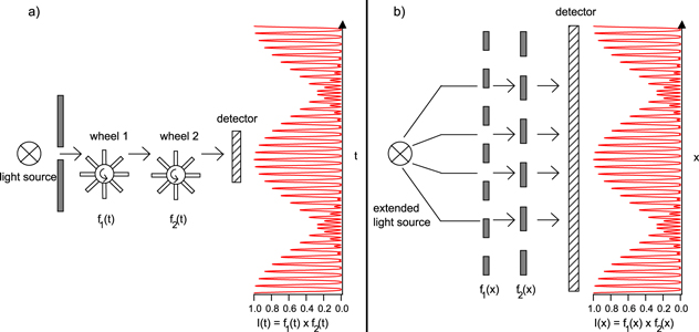
Figure 1. Optical analogue of a one dimensional moiré pattern. (a) Moiré pattern in time space I(t): two turning wheels with spokes are situated in the light path between an emitting point source and a detector. The modulation functions of both wheels are f1(t) and f2(t), the resulting intensity at the detector equals f1(t) × f2(t). (b) Moiré pattern in real space I(x): two semitransparent lattices situated between a spatially extended light source and a spatially extended detector lead to an equivalent modulation function f1(x) × f2(x) in real space. The exact solutions using cosine type modulation functions fi (see text) are sketched in the corresponding I(t)- or I(x)-plots.
Download figure:
Standard image High-resolution imageThe properties of a moiré pattern in real space can be analyzed by transferring this picture to spatially modulated signals as shown in figure 1(b). Here, the two modulators represent the intensity variation of a spatially extended light source, which illuminates two modulators with a spatially extended detector behind them. The modulators may be thought as two transparent foils on which periodic patterns f1(x) and f2(x) are printed that modulate the signal intensity behind the two foils. The observed pattern on the spatially extended detector has the same properties as the detected signal in time space of the setup in figure 1(a), when exchanging the time coordinate t with the real space coordinate x.
Using the function  for the description of each periodic intensity modulator (intensity variation between 0 and 1), we can calculate the signal at the detector
  as:
as:
Although the product f1(x) × f2(x) is a slightly more complicated function then a simple beat [47], it contains a beating term with the spatial frequency k1 − k2. As was noticed already by N'Diaye et al, this term is responsible for the one-dim moiré pattern of the chosen example leading to the mentioned equation  [32]. Expressing cos(k x) as 0.5 × (eikx
− e−ikx) we can list all occurring spatial frequencies of both modulation functions f1(x) and f2(x) and their product as compiled in table 1.
[32]. Expressing cos(k x) as 0.5 × (eikx
− e−ikx) we can list all occurring spatial frequencies of both modulation functions f1(x) and f2(x) and their product as compiled in table 1.
Table 1. Frequencies and amplitudes of the modulation functions fi(x) and the detector signal f1(x) × f2(x) corresponding to the exact solution (2) of the problem sketched in figure 1(b).

|
|

|
|||
|---|---|---|---|---|---|
| Frequency ki | Amplitude | Frequency ki | Amplitude | Frequency ki | Amplitude |
| 0 | 0.5 × 1 | 0 | 0.5 × 1 | 0 | 0.25 × 1 |
| ±k1 | 0.5 × 1/2 | ±k2 | 0.5 × 1/2 | ±k1 | 0.25 × 1/2 |
| ±k2 | 0.25 × 1/2 | ||||
| ±(k1 − k2) | 0.25 × 1/4 | ||||
| ±(k1 + k2) | 0.25 × 1/4 | ||||
Instead of performing the Fourier analysis of the product function f1(x) × f2(x) we can extract the frequency spectrum of the detector signal by a geometric construction that requires solely the knowledge of the two spectra F{fi }(k) corresponding to each modulation function fi as shown in figure 2.

Figure 2. Geometrical construction of the frequency spectrum of the product function f1(x) × f2(x) according to the convolution theorem of Fourier transformation. Shifting the spectra on the k-axis until two peaks of both frequency spectra F{f1} and F{f2} coincide, leads to translation vectors which occur as peaks in the spectrum of the product function F{f1 × f2}. Their amplitudes are calculated by multiplying the amplitudes of the two coinciding peaks. The case of the example according to equation (2) with the frequencies listed in table 1 is plotted for modulating frequencies k1 and k2 as 10 and 9 arbitrary units.
Download figure:
Standard image High-resolution imageIn the two upper panels of figure 2 the frequency spectra of both modulation functions f1(x) and f2(x) are displayed. According to the convolution theorem of Fourier transformation the frequency spectrum of the detector signal equals:

This fact can be used to construct the frequency spectrum of the detector signal by a simple geometric construction when knowing the spectra of the two modulation functions only.
Since the functions listed in table 1 relate to delta distributions in Fourier space at the indicated frequencies ki , the convolution integral in equation (3) leads to non vanishing values only if the two spectra F{f1}(k) and F{f2}(k) are shifted in k-space with respect to each other until their delta distributions match (i.e. their frequency peaks coincide). The applied translation vectors appear as frequencies in the spectrum of the product function. Their corresponding amplitudes equal the product of the amplitudes of the two coinciding frequency peaks. Arrows in figure 2 indicate the k-space shifts which result in observable frequencies of the detector signal. Plotting the resulting amplitudes versus the applied frequency shifts leads to the spectrum of the detector signal as shown in the lowest panel of figure 2. All frequencies and amplitudes obtained by the described geometrical construction in k-space are in full agreement with the listed values of table 1.
3. Fourier frequency analysis of two dimensional moiré patterns—graphene on hexagonal substrate lattice
We can now generalize this concept for two dimensional patterns to mimic the moiré formation of a graphene lattice on a TM-substrate. In this publication, we restrict ourselves to the case of graphene on a TM substrate with a hexagonally arranged surface layer, considering a g-lattice that is rotated by an angle φ with respect to the underlying substrate lattice. The functions that generate the g- and TM-lattice are called fg and fTM, the function of the modulation pattern is fM
= fg × fTM. Their Fourier transforms F{fg}, F{fTM} and F{fM
} = F{fg × fTM} = F{fg}⊗F{fTM} relate to spatial frequencies that are represented as vectors in the reciprocal space plane. They are called  ,
,  and
and  for the g- and TM-lattice as well as for the modulation pattern. The spatial frequency
  describes the unit cell of a possible moiré lattice that can be indexed by vectors (r,s)g and (m,n)TM, relating to the hexagonal unit cell of the g- and the TM-lattice, respectively. The frequency analysis can be restricted to primitive hexagonal lattices, although graphene represents a honeycomb lattice with two atoms per unit cell. Since a honeycomb lattice can be regarded as the sum of two spatially displaced primitive hexagonal lattices and since the Fourier transform is linear, only the amplitudes (intensities) of the occurring frequencies change when considering both displaced lattices, but new frequencies will not occur—a fact well known from crystallography that has been noted as well in the analysis of Hermann [45]. The same argument holds for the effect of deeper substrate layers which are spatially displaced with respect to the topmost substrate lattice and which will complicate the real space pattern but will not introduce new spatial frequencies of the two dimensional projected pattern. Thus, we can restrict ourselves to the case of two primitive hexagonal lattices fg and fTM.
In order to allow a systematic frequency analysis, we choose the following lattice function for the description of a hexagonal lattice with lattice constant a:
The scaling of the function is chosen in a way that f varies between 0 and 1 within the unit cell. The function f contains exclusively zero and first order spatial frequencies. Lattices formed by the nth power of f contain spatial frequencies up to the nth order. Table 2 lists the occurring spatial frequencies ki and their amplitudes for f, f2 and f3. For simplicity, we will call theses functions nth order lattices in the following.
Table 2. Amplitudes of the nth order (n = 1 − 3) spatial frequencies in the Fourier transform of the used lattice functions fn .
Spatial frequencies 
|
|||||||
|---|---|---|---|---|---|---|---|

|
 , ,  , ,  , ,  , ,  , , 
|
 , ,  , ,  , ,  , ,  , , 
|
 , ,  , ,  , ,  , ,  , , 
|
 ,... ,... |
 ,... ,... |
||
 : : |
Amplitude 
|
3 | 1 | ||||
 : : |
Amplitude 
|
15 | 8 | 2 | 1 | ||
 : : |
Amplitude 
|
93 | 60 | 24 | 15 | 3 | 1 |
Figure 3 displays the real space image of these three functions (left panels). The images of their two dimensional Fourier transforms (right panels) reflect the spatial frequencies of the patterns in the reciprocal space plane. Two findings should be noted: (a) all real space patterns generated by the functions f, f2 and f3 are lattices containing the translational symmetry of a primitive two dimensional hexagonal lattice. (b) The introduction of higher order frequencies induces additional spots in the reciprocal space image, but does not change the real space lattice constant. It only results in more localized spots at the real space lattice positions. If delta functions were used to mimic the atom positions of the real space lattice, the reciprocal space image would contain ∞-order spots similar to a low energy electron diffraction (LEED) pattern.
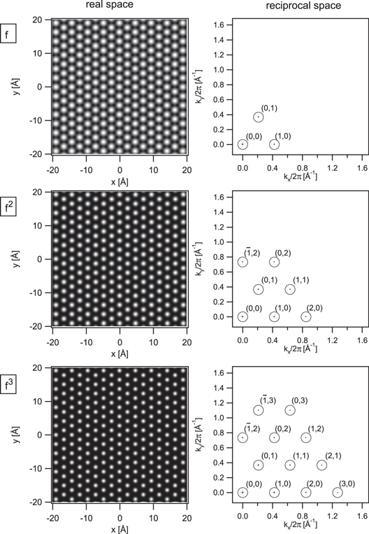
Figure 3. Real space- and reciprocal space images of the hexagonal lattice functions f, f2 and f3 which are used for the frequency analysis of a two dimensional moiré pattern. For the displayed lattices the lattice constant a = 2.715 Å of the Ir(111) surface was chosen. The gray scaling of all real space images ranges from 0 to 1. Due to the large amplitude variation of the spatial frequencies corresponding to the three lattice functions (see table 2), the gray scaling of each reciprocal space plane pattern was adjusted separately.
Download figure:
Standard image High-resolution imageThe calculation of the product fg × fTM of the two lattice functions with different lattice constants ag and aTM in two dimensions leads to a real space image that reflects the optical pattern generated by the two lattices in the geometry of figure 1(b). As noted by N'Diaye et al the resulting two-dim pattern has many properties of a moiré lattice [32, 43, 45]. The spatial frequencies occurring in the modulation pattern can be calculated by a two dimensional Fourier transform and the influence of first- or higher order spatial frequencies on the pattern can be systematically monitored by using one of the functions f, f2 and f3 for the description of the lattices fg and fTM.
We can now discuss the properties of the moiré resulting from of the modulation pattern fg(φ) × fTM using the lattice functions of different order for both lattices. We start the analysis discussing two lattices with lattice constants of 2.715 Å (TM = Ir) and 2.46 Å (g), where both lattices are aligned (φ = 0°) with respect to each other, which applies for the so called R0°-moiré observed for g-Ir(111) [10, 32]. Figures 4 (a) and (b) show the real- and reciprocal space image of the corresponding fg × fTM pattern using f and f2 as lattice functions.
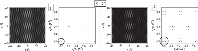
Figure 4. Real and reciprocal space image of the fg × fTM pattern using the first- and second order functions f (left panels) and f2 (right panels) for the description of the lattices. The lattices are oriented in real space with the closed packed direction along the vertical axis so that in reciprocal space the spatial frequencies are aligned horizontally. The circle surrounding the (0,0) spot emphasizes the frequencies that account for the long wave length beating of the moiré pattern. Lattice constants: 2.715 Å (TM = Ir(111)) and 2.460 Å (g).
Download figure:
Standard image High-resolution imageBoth real space patterns show very well the moiré unit cell with a size close to (10 × 10)-g units or (9 × 9)-Ir units, respectively. As expected, due to the rotational alignment of both lattices the moiré cell is also aligned along the crystallographic directions of both hexagonal lattices. In the Fourier transform of the modulation patterns clearly a small hexagon appears close to the (0,0)-spot (emphasized by the circle in reciprocal space plane). This small hexagon relates to K-vectors that describe the largest periodicity of the real space pattern, or the size of the moiré unit cell. The addition of higher order frequencies to the lattice function leads to satellite spots in the reciprocal space image, but does not modify the size of the smallest hexagon, i.e. it does not modify the size of the moiré unit cell but only increases the contrast in the real space image (see right panel of figure 4). It should be noted that due to the rotational alignment of both lattices, the fg × fTM pattern obeys the translational symmetry of a hexagonal lattice, if the lattice constant ratio ag:aTM is a rational number (commensurable coincidence pattern).
Similarly to the geometric construction in reciprocal space outlined above for one dimension, we can use the convolution theorem of Fourier transformation to construct the occurring spatial frequencies of the fg × fTM pattern and calculate the size of the moiré unit cell. This geometric construction is shown in figure 5 for two aligned hexagonal lattices with lattice constants ag and aTM that contain only first order spatial frequencies. The left panel shows the spatial frequencies of the fg- and the fTM-lattice only. They appear as (0,0) and (1,0) and symmetrical equivalent spots in the Fourier transform F{fTM} and F{fg} (red crosses and blue circles). Since we used for both lattices the functions f according to equation (4), the spatial frequencies correspond to delta distributions in reciprocal space. Applying the convolution theorem, all spatial frequencies of the product pattern fg × fTM that appear as spots in its Fourier transform F{fg × fTM} can be traced back to a translation of the two Fourier transforms F{fg} and F{fTM} in reciprocal space: whenever a translation is performed so that a spot of the F{fg}-pattern coincides with one of the F{fTM}-pattern, a spot appears in the Fourier transform F{fg × fTM}at the position of the translation vector in k-space. The resulting pattern is plotted in the right panel of figure 5.
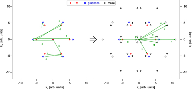
Figure 5. Geometrical construction of the spatial frequencies of the fg × fTM-pattern. Left panel: (0,0) and first order spots of the Fourier transforms F{fg} and F{fTM} correspond to spatial frequencies of the first order lattice functions fg and fTM (TM-lattice: red crosses, g-lattice: blue circles, lattice constants chosen as ag:aTM = 5:6). Right panel: translation vectors connecting spots of the F{fg }- with the ones of the F{fTM}-pattern lead to spots of the Fourier transformed product pattern F{fg × fTM} (new occurring spots are sketched as black diamonds). For sake of visibility, for each translation vector (a)–(h) only one of its six symmetrically equivalent vectors is shown (green arrows).
Download figure:
Standard image High-resolution imageApart from the (0,0)-spot, eight translation vectors and their symmetrical equivalents appear as 48 (=8 × 6) spots in the reciprocal space pattern. 36 (=6 × 6) of them lead to new spatial frequencies (sketched as black diamonds) other than the ones belonging to the two lattices fg and fTM. In figure 5 one of each symmetrically equivalent translation vector is explicitly indicated by a green arrow (a–h). Comparison of figure 5 with the Fourier transform of the first order lattice coincidence pattern in figure 4 shows that the performed geometric construction exactly reproduces all spatial frequencies of the fg × fTM-pattern. All spatial frequencies for the case when using 2nd order lattice functions f2 can be obtained by the same procedure in a similar manner. Drawing our attention to the lowest spatial frequencies of the fg × fTM-pattern, we can now calculate the k-space vectors forming the small hexagon close to the (0,0)-spot as a result of the outlined geometric construction (see vector b in figure 5). Since they relate to the size of the moiré unit cell, we can obtain the unit cell vectors of the moiré in k-space as symmetrically equivalent to:

These frequencies reflect the beating terms responsible for the already mentioned R0° moiré pattern found for graphene on Ir(111). Solving the corresponding formula leads to the moiré structures reported by N'Diaye et al and Hermann [32, 43, 45]. When rotating the graphene layer slightly with respect to the underlying lattice, the orientation and the size of the moiré changes accordingly. Figure 6 displays the case where the pattern fg(φ = 1°) × fTM is plotted for the first- and second order lattice functions f and f2. Both real space images show that the size of the moiré changes slightly, while the orientation of the moiré cell rotates with an amplified rotation speed, as has already been noted [32, 43]. As indicated by the circle in the Fourier transform images both effects are related to the modification of the small hexagon in the reciprocal space plane, which can be analytically calculated by solving equation (5) (see the appendix).
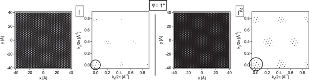
Figure 6. Real and reciprocal space image of the fg(φ = 1°) × fTM -pattern using first and second order lattice functions f (left) and f2 (right) for the description of the lattices. The augmented rotation of the moiré units upon the rotation of the graphene lattice by φ = 1° is easily observed. The corresponding spatial frequencies close to the (0,0)-spot are emphasized by the circle in the reciprocal space panels. Lattice constants: 2.715 Å (TM = Ir(111)) and 2.460 Å (g).
Download figure:
Standard image High-resolution imageWhen increasing the rotation angle φ the real space coincidence pattern fg(φ) × fTM turns surprisingly complex. Its Fourier transform contains the spatial frequencies of each lattice fg and fTM as well as their difference vectors according to the building principle outlined above. When using lattice functions fg and fTM with higher order frequencies, the reciprocal space pattern F{fg(φ) × fTM} turns more complex containing a variety of spatial beating frequencies. But again, all appearing spatial frequencies can be calculated applying the same strategy leading to analytic expressions that describe the size of the moiré unit cell. We will discuss this case when approaching a rotation angle of ∼30° with the help of figure 7 that shows the fg(φ) × fTM-pattern at a rotation angle of φ = 29.6° using first- and second order lattices and lattice parameters that relate again to the g-Ir(111) system applying for the so called R30°-moiré [10].
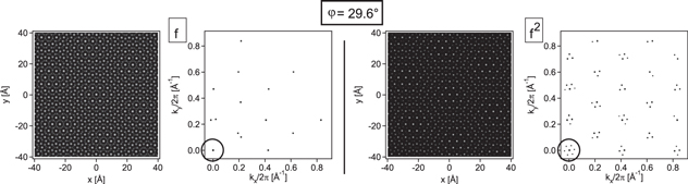
Figure 7. Real and reciprocal space image of the fg(φ = 29.6°) × fTM-pattern using first and second order lattice functions f (left) and f2 (right) for the description of the lattices. The main motif in the pattern of the first- and second order pattern is an approximate  unit cell that is caused by the corresponding spatial frequencies in the Fourier transform. When introducing 2nd order frequencies to the lattice functions, a prominent moiré frequency occurs which is reflected by the small hexagon close to the (0,0)-spot in reciprocal space (emphasized by the circle in the reciprocal space planes). This frequency accounts for the moiré cell in the real space image that clearly appears, when using 2nd order lattice functions (see right panels). Please note that all patterns do not obey the translational symmetry of a lattice but in fact are chiral structures resulting from the handiness of the rotation (see text). Lattice constants: 2.715 Å (TM = Ir(111)) and 2.460 Å (g).
Download figure:
Standard image High-resolution imageThe reciprocal space images of figure 7 show that for first and second order lattices spatial frequencies approach the  positions of the reciprocal lattice. As a result, a pronounced
  motif is observed as spots in
  registry in the real space pattern. On the other hand, close inspection of figure 7 shows that all spatial frequencies are located close to but not precisely at the
  positions of the reciprocal space pattern and thus, this approximate motif does not reflect the unit cell size of the experimentally observed R30°-moiré for which Loginova et al determined a much larger unit cell size in a combined low energy electron microscopy and STM study [10]. The authors distinguished between the approximate coincidence lattice (visible in the LEED pattern) and the moiré unit cell observed by STM. The analysis of figure 7 clarifies why this is the case: the real space pattern shows that beside the strong
  -motif a moiré beating with a much larger wavelength exists, similar in size and orientation as the one of the R0°-moiré (see figure 4). The contrast of this cell in the real space image is much more pronounced when using the 2nd order function f2 for the description of the two coincidence lattices. The spatial frequencies that account for the contrast appear as a small hexagon in the Fourier transform of the 2nd order lattice pattern, accordingly. Its absence and presence for first and second order lattices is emphasized by the circle in the corresponding reciprocal space charts of figure 7. Similar to the construction of the moiré cell of the R0°-moiré, we can now relate the occurrence of all spatial frequencies to difference vectors in k-space of the two rotated lattices. The construction of the particular moiré beating term leading to the small hexagon in figure 7 is imaged in the upper panels of figure 8, displaying the two corresponding reciprocal lattices that are rotated with respect to each other by 29.6°. Here, spatial frequencies of the two rotated lattices are sketched as red crosses (TM = Ir(111)) and blue circles (g) up to the third order. The construction of the moiré beating terms leading to the R30°-moiré is explicitly shown in two inserted charts, where the moiré related spots are drawn as black diamonds.
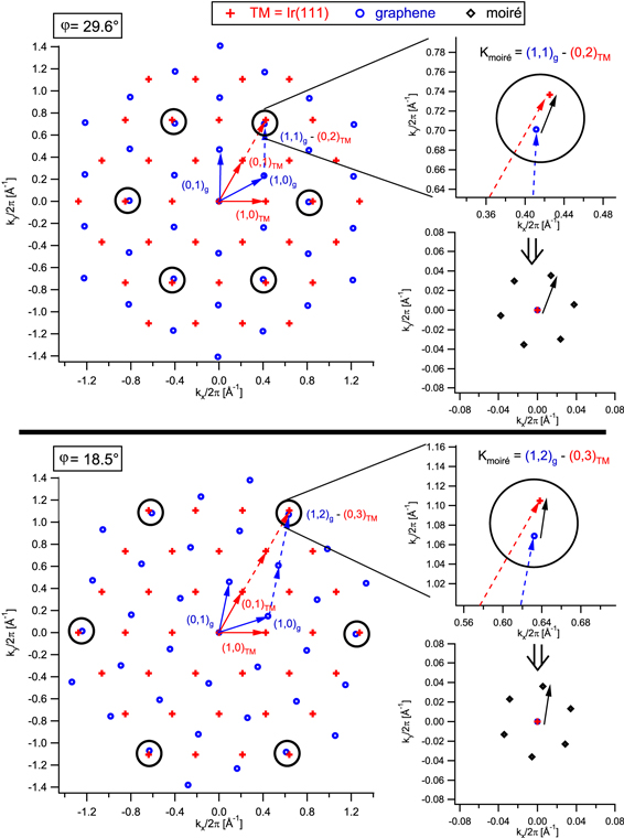
Figure 8. Upper panel: geometric construction of the beating terms which account for the R30°-moiré of g-Ir(111). Due to the rotation of the g lattice with respect to the Ir lattice by 29.6° the (1,1)g and (0,2)Ir-spot almost meet in k-space. Their difference vector accounts for the moiré beating frequency. Lower panel: equivalent geometric construction of beating frequencies leading to the R18.5°-moiré of g-Ir(111). Due to the rotation of the g lattice by 18.5° the (1,2)g and (0,3)Ir-spot almost meet in k-space. Their difference vector leads to the observed moiré wave length. Lattice constants: 2.715 Å (TM = Ir(111)) and 2.460 Å (g).
Download figure:
Standard image High-resolution imageAs indicated in the graphs, due to the rotation of the two lattices by 29.6° the  - and the
  -spot almost meet in k-space. Their difference leads to one of the k-vectors of the small hexagon that appears close to the (0,0)-spot in the reciprocal space plane of the F{fg(φ = 29.6°) × fTM}-pattern. Thus, the condition for the moiré cell of the R30°-moiré is:

Similar to the case of the R0°-moiré pattern, we can relate the identified spatial frequencies to the moiré motif that appears as the long wavelength beating in the real space image of the fg(φ = 29.6°) × fTM-pattern (see figure 7). The displayed construction explains, why this beating frequency is observed at high contrast only when larger than first order lattice functions are used. The construction also shows that when adding higher then 2nd order Fourier components to the lattice functions, no smaller k-vectors than the ones belonging to the small hexagon result from difference terms of the spatial frequencies. I.e., considering larger than 2nd order lattice functions fg(φ) and fTM does not modify the size of the small hexagon but adds satellite spots to it only. As a result, it does not modify the size of the R30°-moiré unit cell, but only increases the contrast of the real space pattern. On the other hand, the addition of third order frequencies to the lattice functions leads to new beating frequencies at a rotation angle φ close to 19.1°. The corresponding construction is shown in the lower panels of figure 8 for a rotation angle φ = 18.5°. The graphs explicitly show that a moiré beating frequency appears, because the  -spot approaches the
  -spot in the reciprocal space plane. The difference vector of the two spatial frequencies accounts for the moiré vector of the fg(φ = 18.5°) × fTM-pattern in k-space. Thus, the condition for the moiré cell of the R18.5°-moiré is:

Again as shown below, the vectors symmetrically equivalent to the one calculated according to equation (7) lead to a small hexagon close to the (0,0)-spot in reciprocal space accounting for the spatial moiré beating frequencies of the corresponding R18.5°-moiré.
So far, our geometric construction led to a sequence of equations (5)–(7) of the form  (or permutations of it). Additional equations can be derived when extending the analysis to even higher orders, following the same building principle: Whenever spatial frequencies of the two rotated lattices approach each other in the reciprocal space plane, a potential moiré pattern appears with a large wavelength. While this analysis can be performed for any order n, we restrict our analytical treatment to the cases n = 1, 2 and 3. As visible from table 2, the amplitudes of the Fourier components of the chosen lattices decrease dramatically with increasing order and as a result, the amplitudes of higher order moiré frequencies are almost not visible in the Fourier transforms of the fg(φ) × fTM-pattern when exceeding n = 3. Restricting the discussion to these three cases seems justified, because it is expected that as well the Fourier expansions of the energy potentials involved lead to energy contributions that have less relevance when increasing the order. In fact, as will be seen below, all discussed moiré structures of the g-Ir(111) and the g-Pt(111) system can be explained by commensurate patterns of first, second and third order.
In the supporting information (available from stacks.iop.org/NJP/16/083028/mmedia) we provide movies that show the gradual development of the fg(φ) × fTM-pattern and its Fourier transform when rotating the graphene lattice counterclockwise by continuously increasing the rotation angle φ from 0° to 60°. The discussed cases of figures 4, 6 and 7 are snapshots of these movies. The data clearly show the effect of the considered order of the lattice on the visibility of the resulting moiré pattern: First order moiré patterns appear with small k-vectors (long wavelength) for φ close to 0° (movie S1a), second order moirés at similar size are visible for φ close to 30° (movie S1b) and third order moirés of similar size appear for φ close to 19.1° (movie S1c). The movies also show that the moiré patterns have certain motifs that do not necessarily reflect the moiré unit cell. As already discussed, the moiré pattern observed for φ close to 30° has a strong ( ) motif, but the large moiré cell clearly appears when considering higher order frequencies for the lattice description. Similarly, the moiré appearing for φ close to 19.1° has a strong (
 ) motif, but again higher order terms are required to evidence the presence of a larger moiré cell. In addition, the real space movies show that for small graphene rotation angles, a moiré pattern appears that seemingly revolves counterclockwise. Depending on the considered order of the pattern, at higher rotation angles φ moiré beatings occur that seemingly reverse their revolution direction towards a clockwise rotation (this is seen in movie S1b for second order moiré at φ exceeding 28° and in movie S1c for the third order moiré at rotation angles above 17°). While the apparent moiré revolution for small angles φ proceeds more than ten times faster than the rotation of the graphene lattice itself, the revolution speed of the higher order moiré beatings proceed at even higher speed. Both effects will be discussed further below.
So far, the performed frequency analysis only calculates where commensurability of the g- and TM-lattice may occur. The fg(φ) × fTM-pattern generally does not contain translational symmetry for an arbitrary rotation angle φ. This results from the fact that cos(φ) and sin(φ) generally lead to irrational numbers which destroys true commensurability. In fact, close inspection of the fg(φ) × fTM-patterns (see figures 6, 7 and the movies in the supporting information) evidences that the apparent unit cells in the real space image generally do not exactly repeat upon translation. One even notices the chirality of the pattern resulting from the counterclockwise rotation of the g-lattice. Nevertheless, the motifs of spatial frequencies are easily observed and we can consider the moiré beatings as the unit cell of a potential commensurate phase. As will be shown in the next paragraphs, if true commensurability occurs, the pattern contains a beating frequency that is part of the graphene- and the substrate lattice. As a consequence, in that case the identified cell is part of the two lattices and obeys their translational symmetry, i.e. a unit cell is defined. In particular, by solving equations (5)–(7), we determine the length and the alignment of the discussed spatial beating frequencies with respect to the substrate (either in reciprocal or in real space). The analytical solutions of the corresponding equations define one of the potential moiré unit cell vectors and are compiled in the appendix of this paper. Due to the symmetry of our problem, two hexagonal lattices rotated by an angle φ with respect to each other lead again to a moiré pattern of hexagonal symmetry. Thus, the two quantities: moiré unit cell length L and its rotation angle Φ with respect to the substrate lattice define size and orientation of the moiré structure.
4. Predicting the size and orientation of potential moiré unit cells
To be more specific, we compare our results with the moiré patterns observed for graphene on Ir(111) which we list in table 3, taking into account the lattice constant aIr = 2.715 Å of the substrate. Table 3 provides the indices of one of the unit cell vectors as used for the matrix notation of the suggested commensurate surface phases and their woods nomenclature relating either to the Ir(111)- or to the graphene lattice. Please note that the corresponding indices are hexagonal sequence numbers referring to equation (1). The rotation of the graphene lattice φ and the rotation Φ of the moiré unit cell with respect to the underlying substrate are given in addition to the graphene lattice constant ag and the relative value of the substrate lattice constant x = aIr/ag that lead to the suggested commensurate unit cells.
Table 3. Experimentally observed moiré patterns for g-Ir(111), their unit cell vectors, rotation angles and lattice constants (lattice constant of Ir(111) = 2.715 Å). (**) While the authors of [32] consider the R0°-moiré as a incommensurate phase with a (9.32 × 9.32)Ir cell, the moiré was also attributed to a phase that ranges between a (19 × 19)Ir and (9 × 9)Ir commensurate phase, depending on the heat treatment of the system. [40] For our discussion, we consider a (9 × 9)Ir and a (10 × 10)Ir unit cell as the two limiting commensurate phases leading to the observed R0°-moiré.
| g-Ir(111) moiré | Unit cell vector (*): (m,n)IrWoods nomenclature | Unit cell vector (*): (r,s)gWoods nomenclature | g-rot. φ [°] | moiré-rot. Φ [°] | ag [Å] |

|
References |
|---|---|---|---|---|---|---|---|
| R0° (**) | (9,0) 
|
(10,0) 
|
0 | 0 | 2.444 |

|
[32, 40] |
(10,0) 
|
(11,0) 
|
0 | 0 | 2.468 |

|
||
| R14° | (4,1) 
|
(4,0) 
|
14 | ∼13.9 | 2.447 |

|
[10, 34] |
| R18.5° | (13,5) 
|
(13,1) 
|
18.5 | ∼22.4 | 2.461 |

|
[10] |
| R30° | (12,2) 
|
(14,9) 
|
29.6 | ∼8.9 | 2.460 |

|
[10] |
(*) or symmetrically equivalent vectors.
We can now discuss the capabilities of our analysis with the help of the four moiré structures that are abbreviated as the R0°-, R14°-, R18.5°- and R30°-moiré in the following. As visible from table 3, a graphene lattice constant ranging between 2.444 Å and 2.468 Å is required in order to achieve commensurability with the Ir(111) substrate in one of the listed moirés. We use these limiting lattice constants to calculate the moiré unit cell length L and rotation angle Φ of the moiré unit cell vector with respect to the substrate as a function of the graphene lattice rotation angle φ and plot both quantities in the panels of figure 9. The red L(φ)- and Φ (φ)-curves are extracted from the solution of the first order equation (5), while the blue curves are calculated by solving the second order equation (6). The green curves describe the moiré cell as expected from the third order equation (7). Since solving these equations also allows computing the trajectories of the corresponding moiré beating frequencies in reciprocal space, we provide a movie in the supporting information that relates to figure 9 and visualizes this motion (movie S2).
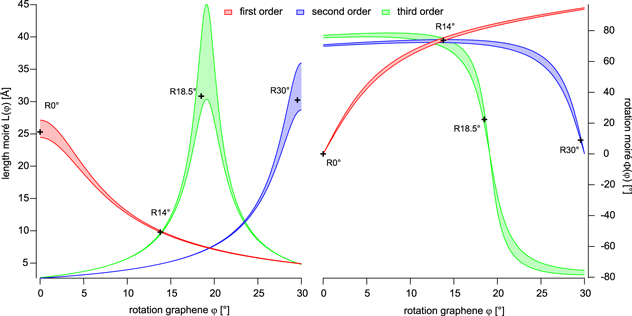
Figure 9. Calculation where possible moiré unit cells may be expected for graphene on Ir(111). The solution of equation (5) (red: first order), (6) (blue: second order) and (7) (green: third order) predicts the length L(φ) and the rotation alignment Φ(φ) of possible moiré unit cells with respect to the substrate lattice as a function of the graphene rotation angle φ. Chosen lattice constants relate to g-Ir(111): 2.715 Å (Ir(111)), upper and lower curves correspond to a graphene lattice constant between 2.444 and 2.468 Å. The indicated crosses mark the cells of the moiré phases listed in table 3 (for the R0°-moiré the (9.32 × 9.32)Ir cell is indicated). Please note that due to the hexagonal symmetry of the system each Φ(φ) curve repeats each 60°. These additional curves were omitted in the graph for the sake of better visibility.
Download figure:
Standard image High-resolution imageLet us start with the solution of the first order spatial frequencies of the moiré pattern (red curves) that lead to the R0°-moiré cell, which ranges between a (10 × 10) and a (9 × 9) cell. The cell size shrinks with increasing rotation angle φ of the graphene layer with respect to the underlying substrate lattice (see red L(φ)-curve). On the other hand the rotation of the graphene lattice induces the rotation of the moiré unit cell. The slope of the Φ(φ)-curve equals ∼ 10 × φ, i.e. the rotation of the moiré cell proceeds about 10 times faster than the turning of the graphene layer. As already noted, the amplified rotation and the shrinkage of the moiré unit cell are clearly visible in the movies S1a, S1b and S1c of the supporting information.
When approaching a graphene lattice rotation angle of φ = 13.9° equivalent first and third order beating frequencies meet at the same point in k-space leading to enlarged amplitudes of the Fourier transform (see movie S2). This spatial periodicity accounts to a moiré length of about  . Since it is compatible with the solution of equation (1), the so called R14°-moiré relates to a commensurate layer with a
  and a (4 × 4)R0° unit cell in Woods notation with respect to the iridium and the graphene lattice, respectively (see table 3).
When further increasing the rotation angle towards φ = 19.1°, the moiré length relating to the third order moiré frequency term approaches its maximum wavelength in real space. This situation corresponds to the case in k-space when the two frequency spots of the graphene and the iridium lattice approach each other (see lower panel of figure 8 for φ = 18.5°). At this rotation angle, the rotation of the graphene layer induces a highly amplified revolution of the third order moiré cell: the slope of the corresponding Φ(φ)-curve equals ∼ 35 × φ. Note, that while the first order moiré cell revolves in the same direction as the rotating graphene lattice, for higher order moiré cells the rotation direction is reversed. This is reflected by the negative slope of the blue and green Φ(φ)-curve in figure 9 and is explicitly seen in the movie S2 of the supporting information. The change of sign of the revolving direction of the higher order moiré frequencies is responsible for the already mentioned seemingly reversed rotation of the moiré pattern, once the rotation angle of φ ∼ 18° is exceeded (movies S1). As also indicated in the graph, the length and orientation of the third order k-space moiré vector at a graphene rotation angle of φ ∼ 18.5° is consistent with the observed R18.5°-moiré structure listed in table 3 (leading to a  unit cell when relating to the Ir lattice). We should note that close to the rotation angle of φ ∼ 18.5° the L(φ)-curve belonging to the first and second order moiré cells cross each other. Since the corresponding Φ(φ)-curves modulo 60° differ only slightly, the trajectories of the corresponding spatial beating frequencies almost cross in reciprocal space when reaching this graphene rotation angle (see movie S2). As a consequence of the almost coinciding beating frequencies, the R18.5°-moiré pattern contains the already mentioned pronounced real space
  motif. Since the crossing of the spatial frequencies is only approximate and the unit cell vectors of this potential
  unit cell do not fulfill equation (1), no commensurability is met and the moiré pattern with the larger
  unit cell is realized according to the third order frequency terms of the lattices.
When reaching a rotation angle φ of ∼23.4°, the second (blue) and third order (green) related curves of figure 9 cross, but no commensurable moiré structure is observed. In fact, close inspection of figure 9 and the trajectories in movie S2 show that again, the crossing of the second and third order frequencies in the reciprocal space plane is only approximate, but not strict (i.e., the crossing of the corresponding L(φ)- and the Φ(φ)-curves in figure 9 takes place at slightly different values for φ). As a result, a similar high symmetry condition as found for the R14°-moiré does not occur at this rotation angle and no moiré pattern is observed.
Finally, at φ ∼ 29.6°, where the second order L(φ)-curve approaches its maximum, a commensurate moiré phase is found with a  unit cell when relating to the Ir lattice (see table 3). The rotation of the graphene layer again induces an amplified revolution of the second order moiré cell at a rotation angle close to 30° in the clockwise direction, which is reflected by the negative slope of the Φ(φ)-curve of ∼ 19 × φ. Thus, the revolution speed of the second order moiré cell ranges between the one of the first and third order moiré cell. Close inspection of figure 9 shows that at this rotation angle the first and third order beating frequency curves cross, which leads to the already discussed
  motif of the R30°-moiré pattern. Again, as in the case of the third order moiré at a rotation angle of 18.5°, the crossing of the corresponding spatial frequencies in reciprocal space is only approximate and equation (1) is not fulfilled so that the commensurate moiré cell is considerably larger than this motif.
We should point out again that figure 9 and the movie S2 show four cases, where spatial beating frequencies of different order meet in k-space. These positions are related to high symmetry cases, where the rotated graphene lattice proceeds along certain directions of the substrate lattice. In particular, the rotation angles of 30°, 23.4°, 19.1° and 13.9° relate to orientations, where the [1,1]-, [3,2]-, [2,1]- and [3,1]-direction of the reciprocal graphene lattice is aligned along a main direction of the substrate lattice. In fact as shown above, close to these high symmetry cases commensurate moirés occur for graphene on Ir(111) (see figure 9) and—as noticed by Loginova et al—the corresponding moiré patterns contain the mentioned specific motifs [10]. On the other hand, e.g. at the angle of φ = 23.4° no commensurate phase is observed for graphene on Ir(111). We will show in the following section, why this is the case, which conditions have to be fulfilled to achieve commensurability and how to compute the unit cell of the corresponding moiré structures.
5. Predicting the size and orientation of commensurate moiré unit cells
So far, we could show that moiré patterns contain spatial beating frequencies with a hexagonal cell characterized by a unit vector  of length L(φ) that is rotated with respect to the [1, 0]-direction of the substrate lattice by Φ(φ). If in addition, the moiré pattern obeys true commensurability, the unit cell vector
  must be a vector of the substrate- and the graphene lattice simultaneously. In this case, it can be expressed by coordinates (m,n)TM and (r,s)g
relating either to the TM substrate or the graphene lattice, respectively. As has been noted in [41], the vector
must be a vector of the substrate- and the graphene lattice simultaneously. In this case, it can be expressed by coordinates (m,n)TM and (r,s)g
relating either to the TM substrate or the graphene lattice, respectively. As has been noted in [41], the vector  of a commensurate cell fulfills equation (1) linking the so called hexagonal number sequences of the substrate (m,n)TM to the ones of the graphene layer (r,s)g
. Since we derived analytic expressions for L(φ) and Φ(φ) (see the appendix of this paper), we can now determine the required integer numbers m, n, r and s. At first, we calculate the length L(φ) in units of the substrate lattice L(φ) = l(φ) × aTM. Describing the unit cell of the substrate with vectors
of a commensurate cell fulfills equation (1) linking the so called hexagonal number sequences of the substrate (m,n)TM to the ones of the graphene layer (r,s)g
. Since we derived analytic expressions for L(φ) and Φ(φ) (see the appendix of this paper), we can now determine the required integer numbers m, n, r and s. At first, we calculate the length L(φ) in units of the substrate lattice L(φ) = l(φ) × aTM. Describing the unit cell of the substrate with vectors  and
and  , we determine the hexagonal sequence numbers (m,n)TM of the moiré unit cell vector
  with respect to the substrate lattice as:

Accordingly, the moiré unit cell vector  also has to be expressed by the coordinates (r, s)g
with respect to the graphene lattice. Using the notation of the rotated coordinate system (rotation angle φ) this leads to:
also has to be expressed by the coordinates (r, s)g
with respect to the graphene lattice. Using the notation of the rotated coordinate system (rotation angle φ) this leads to:

Here, the parameter x = aTM/ag expresses the relative lattice constant of the substrate and the graphene layer. Solving equations (8) and (9) leads to the exact solution for  = (m, n)TM and
  = (r, s)g:

and:

By inserting l(φ) and Φ(φ) from the spatial frequency analysis (the analytic functions are given in the appendix of this paper) into equations (10) and (11), we can determine the values for m, n, r, s as functions of x and φ, i.e. m = m(x, φ), n = n(x, φ), r = r(x, φ) and s = s(x, φ). The last condition to be fulfilled for commensurability requires that all numbers m, n, r and s are integers. This construction can be regarded as the solution of a geometrical problem. We can consider each of the four equations, e.g. the m = m(x, φ) as a surface above the (x, φ)-plane. The iso-height curves of the m(x, φ) surface can be thought as contour traces in the (x, φ)-plane, which are of particular interest when their height amounts an integer number. For the case of first-order moirés we can solve the equations of the type m(x, φ) = const. as the roots of a second order polynom. The analytic expressions of these contour traces are listed in the appendix of this paper. For higher order moiré patterns they are roots of a 4th order polynom and the iso-height contour traces are numerically calculated. Commensurability of the rotated graphene layer with the underlying hexagonally packed support surface is achieved, if the contour traces of the m = m(x, φ), n = n(x, φ), r = r(x, φ) and s = s(x, φ) surface cross each other in the (x, φ)-plane and are thus solutions of equations (10) and (11). As a consequence, the graphical solution of the crossing points of the integer iso-height traces in the (x, φ)-plane represent the commensurate nth order moirés in the (x, φ)-parameter space. The corresponding integer tuples (m, n) and (r, s) are the coordinates of the corresponding moiré unit cell vector in the coordinate system of the TM- and the graphene lattice, respectively. In order to visualize this solution, we calculate the absolute deviation of the m(x, φ)-surface from its nearest integer number, i.e. we calculate abs[m-round(m)]. If we add the corresponding terms for m, n, r and s, we obtain a hill and valley function above the (x, φ)-plane that amounts zero, if a commensurate moiré cell can be geometrically realized. Such plots are shown in figure 10 for first, second and third order moiré cells.
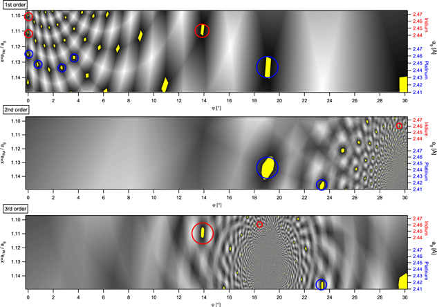
Figure 10. Commensurability plots for 1st, 2nd and 3rd order moiré patterns. Yellow patches indicate where the conditions for commensurability between the graphene and substrate lattice are met. Circles indicate the cases, where moiré patterns are experimentally observed for g-Ir(111) (red) and g-Pt(111) (blue) (see tables 3 and 4). The left axis indicates the ratio of the lattice constants x = aTM/ag. On the right, the corresponding lattice constant of the graphene layer ontop of Ir(111) (red) and Pt(111) (blue) is shown.
Download figure:
Standard image High-resolution imageIn agreement with the findings of the last paragraphs, the obtained commensurability plots show that first order moirés mainly lead to commensurate phases at rotation angles φ close to 0°, whereas the second order moiré leads to 2nd order commensurate phases mainly at rotation angles close to 30° and many of the third order moiré phases are found commensurable close to 19.1°. In addition, we can now focus on the x-parameter dependency, which represents the relative lattice constants of the substrate and the graphene lattice. The right axis of figure 10 displays the absolute graphene lattice constant that corresponds to the x-value if the graphene resides on an Ir(111) surface (red scale) and on Pt(111) (blue scale). We can now discuss where commensurate moiré phases are expected for the two systems, since only moderately strained graphene layers seem probable candidates for CVD grown moiré phases. In addition, figure 10 emphasizes by red and blue circles where moiré cells are experimentally observed on Ir(111) and on Pt(111) (see as well table 3 and below table 4). The displayed commensurability plot clearly shows that, depending on the combined lattice constants, certain moirés may occur on a specific TM surface, but may not be found on a support with a different lattice constant. In particular, the plots show that a R14°-moiré should occur for graphene grown on Ir(111) that is not expected on Pt(111), whereas the situation is reversed for the R23.4°-moiré. In order to show the universality of the provided solution we show zooms of the parameter space of the moirés of different order in figure 11. Here, we also added the contour traces belonging to the (m,n) and (r,s) tuples of the corresponding commensurate cells.
Table 4. Experimentally observed moiré patterns for g-Pt(111), their unit cell vectors, rotation angles and the corresponding lattice constants (lattice constant of Pt(111) = 2.77 Å). (**) In [15] only the unit cell with respect to the graphene lattice was identified. The corresponding cell with respect to the Pt lattice results from the commensurability plots of figure 11. Table 4 also indicates the order of commensurability of the moiré cells as it follows the concept of the graphs in figure 11.
| g-Pt(111) moiré | Unit cell vector(*): (m,n)PtWoods nomenclature | Unit cell vector(*): (r,s)gWoods nomenclature | g-rot. φ [°] | moiré-rot. Φ [°] | ag [Å] |

|
Order | References |
|---|---|---|---|---|---|---|---|---|
| R23.4° | (5,2) 
|
(5,0) 
|
23.4 | 23.4 | 2.415 |

|
2 + 3 | [12, 15] |
| R19.1° | (2,3) 
|
(3,0) 
|
19.1 | 19.1 | 2.443 |

|
1 + 2 | [14, 15] |
| R3.7°(**) | (8,4) 
|
(9,4) 
|
3.7 | 30 | 2.443 |

|
1 | [15] |
| R2.7° | (8,3) 
|
(9,3) 
|
2.7 | 21.8 | 2.443 |

|
1 | [15] |
| R0.8°(**) | (8,1) 
|
(9,1) 
|
0.8 | 6.6 | 2.443 |

|
1 | [15] |
| R0° | (8,0) 
|
(9,0) 
|
0 | 0 | 2.462 |

|
1 | [12] |
(*) or symmetrically equivalent vectors.
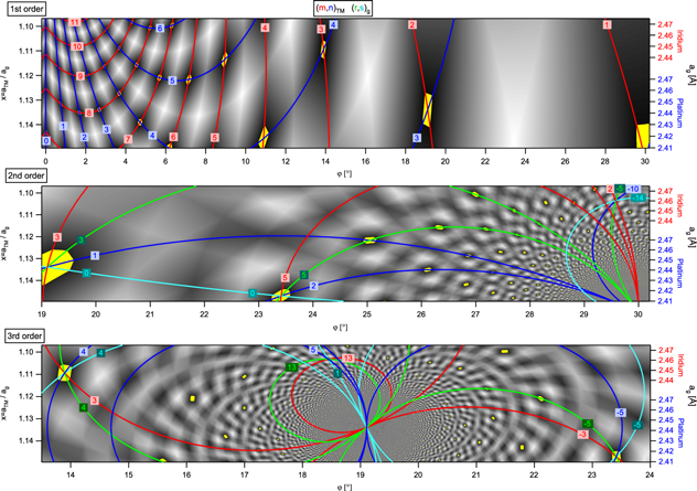
Figure 11. Commensurability plot for 1st, 2nd and 3rd order moirés including the (m, n)TM, (r, s)g contour plots. The graphs show zooms into special regions of interest of the parameter space of g-Ir(111) and g-Pt(111). The indicated colored numbers refer to the indices relating to their corresponding contour traces. For first order commensurate cells, the (m, n)TM contour traces coincide with the (r = m + 1, s = n)g contour lines so that commensurable phases are possible if two traces cross each other. In order to achieve higher order commensurability four different (m, n)TM- and (r, s)g-traces have to cross each other. While the first order plot shows all traces, in the second order graph only the traces are indicated that lead to the (3,1)TM (3,0)g-, the (5,2)TM (5,0)g- and the (2,−10)TM (−5,−14)g-moiré. In the third order graph, only the traces are displayed that belong to the (3,4)TM (4,4)g-, the (13,5)TM (13,1)g- and the (−3,−5)TM (−5,−5)g-moiré.
Download figure:
Standard image High-resolution imageThus, the displayed contour traces allow the identification of the commensurate moiré unit cells. When comparing with the data of table 3, one easily sees that all listed commensurate graphene moiré cells on Ir(111) are found in the graphs of figure 11 in agreement with the determined moiré unit cells: the (9,0)Ir and the (10,0)Ir cell (R0°-moiré) are evidenced as first order commensurate phases, the (4,1)Ir cell (R14°-moiré) is symmetrically equivalent to (3,4)Ir and thus found as a first and third order commensurate phase, the (13,5)Ir cell (R18.5°-moiré) is found in the third order plot and the (12,2)Ir cell (R30°-moiré), being symmetrically equivalent to the (2,−10)Ir cell belongs to a second order commensurate phase. The agreement in the unit cell notation with respect to the graphene lattice can be found in a similar way. Thus, figure 11 clearly shows the value of our geometric construction of moiré beating frequencies. We can use the same graph to consider the observed moiré cells of the g-Pt(111) system which we list in table 4.
Again, figure 11 proves that all listed moiré cells appear with the correct unit cell notation. Please note that (5,2)Pt (R23.4°-moiré) is symmetrically equivalent to (−3,−5)Pt, that (2,3)Pt (R19.1°-moiré) is symmetrically equivalent to (3,1)Pt and that the vectors indexing the R3.7°-, R2.7°-, R0.8°- and R0°-moiré are found in figure 11 with the same notation as in table 4. Also, all corresponding vectors relating to the graphene lattice are correctly indexed by our analysis. In addition, we can determine the order of commensurability that leads to the moiré unit cells with the help of figure 11. Inspection of the 1st, 2nd and 3rd order commensurability plot shows that the R23.4°-moiré is a result of a 2nd and 3rd order commensurate phase and that the R19.1°-moiré belongs to a unit cell which is commensurable with respect to the 1st and 2nd order simultaneously. The corresponding values were added to table 4. As already noted above, the plots displayed in figure 11 indicate the cells that fulfill equations (10) and (11) as the requirements for commensurability and thus explain, why for graphene on Pt(111) the R23.4°-moiré appears, which is absent for g-Ir(111) and why this situation is reversed for the R14°-moiré. We should note that in the literature of graphene grown on different TM substrates sometimes moiré unit cells are suggested that require an extreme straining of the graphene lattice and therefore appear rather unlikely. Our analysis related to the displayed commensurability plots of figures 10 and 11 provides a strategy for discussing such cases, which will be the topic of a forth coming paper.
6. Conclusion
With the help of the outlined geometric construction we can analytically determine the spatial beating frequencies that lead to the formation of a moiré pattern caused by two coinciding lattices. Our model can be applied for moirés that result from the spatial beating of two hexagonal lattices, such as graphene placed on transition metal support surfaces with hexagonal symmetry. We explicitly solve the case when such moirés result in first, second and third order commensurate phases and show how to extend the analysis when even higher order commensurability is of interest. As a result, we are able to predict the expected commensurate phases for graphene on any hexagonally arranged support surface, which is tested for the moiré patterns found for graphene on Ir(111) and on Pt(111). In particular, our model explains why certain moirés have strong spatial motifs that do not necessarily lead to a commensurate phase, whereas others do. Our analysis can be applied for graphene, h-BN or other sp2-networks on any hexagonally arranged support surface. It provides the strategy how to critically discuss moiré cells of such systems that were reported in the literature.
Acknowledgment
This work was supported by the German Research Foundation (DFG) in the framework of the Priority Program 1459 'Graphene'.
Appendix A
A.1. Size and orientation of spatial moiré beating frequencies
In this section we compile the solutions of equations (5)–(7) which were used for the calculation of the curves in figure 9 and the trajectories of the spatial frequency spots in k-space in movie S2 which can be found in the supporting information. We use the following abbreviations: aTM = lattice constant of support, x = aTM/ag (ratio of support- and graphene lattice constant), φ = rotation angle of the graphene lattice with respect to the one of the support lattice. Due to the sixfold symmetry of the problem the definition of the graphene and moiré rotation angle allows some freedom. We calculate the moiré rotation angle for the case of a counterclockwise rotation of the graphene lattice with respect to one of the main crystallographic axis of the support lattice. The clockwise rotation can be calculated if the indices of the corresponding vectors are exchanged. The vectors, where mixed indices are used reflect the solutions where the rotation angles are added to or subtracted from 60°.
A.1.1. First order beating frequency—solution to equation (5): 

Length of the moiré unit cell in reciprocal space:
Length of the moiré unit cell in real space:
Rotation angle of the moiré cell with respect to the support lattice:
A.1.2. Second order beating frequency—solution to equation (6):
Length of the moiré unit cell in reciprocal space:

Length of the moiré unit cell in real space:

Rotation angle of the moiré cell with respect to the support lattice:
A.1.3. Third order beating frequency—solution to equation (7):
Length of the moiré unit cell in reciprocal space:

Length of the moiré unit cell in real space:

For the rotation angle of the moiré cell Φ with respect to the support lattice, we have to consider two cases, since the occurring values for Φ exceed the principal value of the arccos-function and we have to extend the function accordingly. The curve x0(φ) in the (x, φ)-parameter plane separating these two case can be analytically determined, when solving the condition, where the argument of the arccos function amounts +1 or −1. The resulting equation is:
Thus, depending on the range within the (x, φ)-parameter space, the rotation angle of the moiré cell Φ has to be determined according to one of the following formula:
and
For the computation of the third order graphs in figures 10 and 11 the above described case separation had to be explicitly taken into account.
A.2. Commensurability plots—iso-height contour traces
For commensurable moirés with the indexing (m, n)TM and (r, s)g we can compute the possible indices by inserting the above listed solutions for l(x, φ) and Φ(x, φ) into equations (10) and (11) leading to functions of the form  ,
,  ,
,  and
and  .
.
A.2.1. First order moirés
For first order moirés, the corresponding iso-height contour traces in the (x, φ) parameter space can be analytically described. They are roots of a second order polynom and can be expressed as functions of the form x(φ, m), x(φ, n), x(φ, r) and x(φ, s):
According to the indexing (m, n)TM with respect to the substrate lattice we have:

and
The contour traces relating to the indexing with respect to the graphene lattice (r, s)g, can be shown to be identical functions with a modified indexing obeying r = m + 1 and s = n. As a consequence, commensurability with respect to the substrate lattice described by a (m, n)TM moiré always relates to commensurability with respect to the graphene lattice according to a (m + 1, n)g moiré.
A.2.2. Higher order moirés
For higher order moirés the  ,
,  ,
,  and
and  functions relate to roots of a 4th order polynom and iso-height traces cannot be determined analytically but have to be numerically computed. Here, the condition of commensurability is fulfilled only if all four contour traces in the (x, φ) parameter space cross each other. This is seen in the commensurability plots of figure 11.