


Abstract
To achieve universal quantum computation via general fault-tolerant schemes, stabilizer operations must be supplemented with other non-stabilizer quantum resources. Motivated by this necessity, we develop a resource theory for magic quantum channels to characterize and quantify the quantum 'magic' or non-stabilizerness of noisy quantum circuits. For qudit quantum computing with odd dimension d, it is known that quantum states with non-negative Wigner function can be efficiently simulated classically. First, inspired by this observation, we introduce a resource theory based on completely positive-Wigner-preserving quantum operations as free operations, and we show that they can be efficiently simulated via a classical algorithm. Second, we introduce two efficiently computable magic measures for quantum channels, called the mana and thauma of a quantum channel. As applications, we show that these measures not only provide fundamental limits on the distillable magic of quantum channels, but they also lead to lower bounds for the task of synthesizing non-Clifford gates. Third, we propose a classical algorithm for simulating noisy quantum circuits, whose sample complexity can be quantified by the mana of a quantum channel. We further show that this algorithm can outperform another approach for simulating noisy quantum circuits, based on channel robustness. Finally, we explore the threshold of non-stabilizerness for basic quantum circuits under depolarizing noise.
Export citation and abstract BibTeX RIS
1. Introduction
1.1. Background
One of the main obstacles to physical realizations of quantum computation is decoherence that occurs during the execution of quantum algorithms. Fault-tolerant quantum computation (FTQC) [1, 2] provides a framework to overcome this difficulty by encoding quantum information into quantum error-correcting codes, and it allows reliable quantum computation when the physical error rate is below a certain threshold value.
The fault-tolerant approach to quantum computation allows for a limited set of transversal, or manifestly fault-tolerant, operations, which are usually taken to be the stabilizer operations (SOs). However, the SOs alone do not enable universality because they can be simulated efficiently on a classical computer, a result known as the Gottesman–Knill theorem [3, 4]. The addition of non-stabilizer quantum resources, such as non-SOs, can lead to universal quantum computation [5]. With this perspective, it is natural to consider the resource-theoretic approach [6] to quantify and characterize non-stabilizer quantum resources, including both quantum states and channels.
One solution for the above scenario is to implement a non-SO via state injection [7] of so-called 'magic states,' which are costly to prepare via magic state distillation [5] (see also [8–14]). The usefulness of such magic states also motivates the resource theory of magic states [15–20], where the free operations are the SOs and the free states are the stabilizer states (abbreviated as 'Stab'). On the other hand, since a key step of fault-tolerant quantum computing is to implement non-SOs, a natural and fundamental problem is to quantify the non-stabilizerness or 'magic' of quantum operations. As we are at the stage of noisy intermediate-scale quantum (NISQ) technology, a resource theory of magic for noisy quantum operations is desirable both to exploit the power and to identify the limitations of NISQ devices in fault-tolerant quantum computation (FTQC).
1.2. Overview of results
In this paper, we develop a framework for the resource theory of magic quantum channels, based on qudit systems with odd prime dimension d. Related work on this topic has appeared recently [21], but the set of free operations that we take in our resource theory is larger, given by the completely positive-Wigner-preserving (CPWP) perations as we detail below. We note here that d-level FTQC based on qudits with prime d is of considerable interest for both theoretical and practical purposes [22–26].
Our paper is structured as follows.
- In section 2, we first review the stabilizer formalism [4] and the discrete Wigner function [27–29]. We further review various magic measures of quantum states and introduce various classes of free operations, including the SOs and beyond.
- In section 3, we introduce and characterize the CPWP operations. We then introduce two efficiently computable magic measures for quantum channels. The first is the mana of quantum channels, whose state version was introduced in [19]. The second is the max-thauma of quantum channels, inspired by the magic state measure in [20]. We prove several desirable properties of these two measures, including reduction to states, faithfulness, additivity for tensor products of channels, subadditivity for serial composition of channels, an amortization inequality, and monotonicity under CPWP superchannels.
- In section 4, we explore the ability of quantum channels to generate magic states. We first introduce the amortized magic of a quantum channel as the largest amount of magic that can be generated via a quantum channel. Furthermore, we introduce an information-theoretic notion of the distillable magic of a quantum channel. In particular, we show that both the amortized magic and distillable magic of a quantum channel can be bounded from above by its mana and max-thauma.
- In section 5, we apply our magic measures for quantum channels in order to evaluate the magic cost of quantum channels, and we explore further applications in quantum gate synthesis. In particular, we show that at least four T gates are required to perfectly implement a controlled-controlled-NOT gate.
- In section 6, we propose a classical algorithm, inspired by [30], for simulating quantum circuits, which is relevant for the broad class of noisy quantum circuits that are currently being run on NISQ devices. This algorithm has sample complexity that scales with respect to the mana of a quantum channel. We further show by concrete examples that the new algorithm can outperform a previous approach for simulating noisy quantum circuits, based on channel robustness [21].
2. Preliminaries
2.1. The stabilizer formalism
For most known fault-tolerant schemes, the restricted set of quantum operations is the SOs, consisting of preparation and measurement in the computational basis and a restricted set of unitary operations. Here we review the basic elements of the stabilizer states and operations for systems with a dimension that is a product of odd primes. Throughout this paper, a Hilbert space implicitly has an odd dimension, and if the dimension is not prime, it should be understood to be a tensor product of Hilbert spaces each having odd prime dimension.
Let  denote a Hilbert space of dimension d, and let
  denote the standard computational basis. For a prime number d, we define the unitary boost and shift operators
  in terms of their action on the computational basis:


where ⊕ denotes addition modulo d. We define the Heisenberg–Weyl operators as

where  .
.
For a system with composite Hilbert space  , the Heisenberg–Weyl operators are the tensor product of the subsystem Heisenberg–Weyl operators:

where  is an element of
  .
.
The Clifford operators  are defined to be the set of unitary operators that map Heisenberg–Weyl operators to Heisenberg–Weyl operators under unitary conjugation up to phases:

These operators form the Clifford group.
The pure stabilizer states can be obtained by applying Clifford operators to the state  :
:

A state is defined to be a magic or non-stabilizer state if it cannot be written as a convex combination of pure stabilizer states.
2.2. Discrete Wigner function
The discrete Wigner function [27–29] was used to show the existence of bound magic states [18]. For an overview of discrete Wigner functions, we refer to [18, 19] for more details. See also [31] for a review of quasi-probability representations in quantum theory, with applications to quantum information science.
For each point  in the discrete phase space, there is a corresponding operator
  , and the value of the discrete Wigner representation of a state ρ at this point is given by

where d is the dimension of the Hilbert space and  are the phase-space point operators:

The discrete Wigner function can be defined more generally for a Hermitian operator X acting on a space of dimension d via the same formula:

For the particular case of a measurement operator E satisfying  , the discrete Wigner representation is defined as

i.e. without the prefactor  . The reason for this will be clear in a moment and is related to the distinction between a frame and a dual frame [30, 32, 33].
Some nice properties of the set  are listed as follows:
- 1.
 is Hermitian;
 - 2.
- 3.
- 4.
- 5.
- 6..


![$\mathrm{Tr}\,[{A}_{{\bf{u}}}{A}_{{\bf{u}}^{\prime} }]=d\,\delta ({\bf{u}},{\bf{u}}^{\prime} );$](https://content.cld.iop.org/journals/1367-2630/21/10/103002/revision2/njpab451dieqn18.gif)
![$\mathrm{Tr}\,[{A}_{{\bf{u}}}]=1;$](https://content.cld.iop.org/journals/1367-2630/21/10/103002/revision2/njpab451dieqn19.gif)


From the second property above and the definition in (7), we conclude the following equality for a quantum state ρ:

For this reason, the discrete Wigner function is known as a quasi-probability distribution. More generally, for a Hermitian operator X, we have that

so that for a subnormalized state ω, satisfying  and
and ![$\mathrm{Tr}\,[\omega ]\leqslant 1$](https://content.cld.iop.org/journals/1367-2630/21/10/103002/revision2/njpab451dieqn23.gif) , we have that
, we have that  .
.
Following the convention in (10) for measurement operators, we find the following for a positive operator-valued measure (POVM)  (satisfying
  and
and  ):
):

so that the quasi-probability interpretation is retained for a POVM. That is,  can be interpreted as the conditional quasi-probability of obtaining outcome x given input
  .
.
We can quantify the amount of negativity in the discrete Wigner function of a state ρ via the sum negativity, which is equal to the absolute sum of the negative elements of the Wigner function [19]:

By definition, we find that  . The mana of a state ρ is defined as [19]

We define the mana more generally, as in [20], for a positive semi-definite operator X via the formula

We denote the set of quantum states with a non-negative Wigner function by  (Wigner polytope), i.e.

It is known that quantum states with non-negative Wigner function are classically simulable and thus are useless in magic state distillation [18], which can be seen as the analog of states with positive partial transpose (PPT) in entanglement distillation [34, 35].
Motivated by the Rains bound [36] and its variants [37–43] in entanglement theory, the set of sub-normalized states with non-positive mana was introduced as follows [20] to explore the resource theory of magic states:

It follows from definitions and the triangle inequality that ![$\mathrm{Tr}\,[\sigma ]\leqslant 1$](https://content.cld.iop.org/journals/1367-2630/21/10/103002/revision2/njpab451dieqn32.gif) if
if  (alternatively one can conclude this by inspecting the right-hand side of (16)).
Furthermore, we define  to be the set of Hermitian operators with non-negative Wigner function:

The Wigner trace norm and Wigner spectral norm of an Hermitian operator V are defined as follows, respectively:


The Wigner trace and spectral norms are dual to each other in the following sense:


with C ranging over Hermitian operators within the same space.
2.3. Stabilizer channels and beyond
A SO consists of the following types of quantum operations: Clifford operations, tensoring in stabilizer states, partial trace, measurements in the computational basis, and post-processing conditioned on these measurement results. Any quantum protocol composed of these quantum operations can be written in terms of the following Stinespring dilation representation: ![${E}(\rho )={{\rm{T}}{\rm{r}}}_{E}[U(\rho \otimes {\rho }_{E}){U}^{\dagger }]$](https://content.cld.iop.org/journals/1367-2630/21/10/103002/revision2/njpab451dieqn35.gif) , where U is a Clifford unitary and the ancilla
, where U is a Clifford unitary and the ancilla  is a stabilizer state.
The authors of [44] generalized the set of SOs to stabilizer-preserving operations, which are those that transform stabilizer states to stabilizer states and which form the largest set of physical operations that can be considered free for the resource theory of non-stabilizerness. More recently, [21] introduced the completely stabilizer-preserving operations (CSPO); i.e. a quantum operation Π is called completely stabilizer-preserving if for any reference system R,

2.4. Magic measures of quantum states


3. Quantifying the non-stabilizerness of a quantum channel
3.1. Completely positive-Wigner-preserving operations
A quantum circuit consisting of an initial quantum state, unitary evolutions, and measurements, each having non-negative Wigner functions, can be classically simulated [30]. It is thus natural to consider free operations to be those that completely preserve the positivity of the Wigner function. Indeed, any such quantum operations are proved to be efficiently simulated via classical algorithms in section 6 and thus become reasonable free operations for the resource theory of magic.
(Completely PWP operation).Definition 1 A Hermiticity-preserving linear map Π is called CPWP if for any system R with odd dimension, the following holds

Figure 1 depicts the relationship between SOs, completely stabilizer-preserving operations, and completely PWP operations.

Figure 1. Relationship between stabilizer operations, completely stabilizer-preserving operations, and completely PWP operations.
Download figure:
Standard image High-resolution imageWe now recall the definition of the discrete Wigner function of a quantum channel from [17], which is strongly related to the Wigner function of a quantum channel as defined in [46, equation (95)].
(Discrete Wigner function of a quantum channel).Definition 2 Given a quantum channel  , its discrete Wigner function is defined as


Here  denotes the Choi–Jamiołkowski matrix [47, 48] of the channel
  , where
  and
and  are orthonormal bases on isomorphic Hilbert spaces
  and
and  , respectively. More generally, the discrete Wigner function of a Hermiticity-preserving linear map
  can be defined using the same formula in (29), by substituting
  therein with
  .
.
From the definition above and the properties recalled in section 2.2, it follows for a quantum channel  that
that

because


where the penultimate equality follows from the fact that  is trace preserving (in fact here we did not require complete positivity or even linearity). Due to the normalization in (30),
  can be interpreted as a conditional quasi-probability distribution.
Furthermore, the discrete Wigner function of a channel allows one to determine the output Wigner function from the input Wigner function by propagating the quasi-probability distributions, just as one does in the classical case. When there is no reference system, such a statement was proved in [17]. Here we slightly extend this result to the case with a reference system in the following lemma.
Lemma 1. For an input state  and a quantum channel
  with respective Wigner functions
  and
and  , the Wigner function
  of the output state
  is given by

Proof. The proof is straightforward:


All steps follow from definitions and the properties of the phase-space point operators recalled in section 2.2. In particular, we made use of the fact that  in the second equality. ■
Theorem 2. The following statements about CPWP operations are equivalent:
- 1.The quantum channel is CPWP;
- 2.The discrete Wigner function of the Choi–Jamiołkowski matrix is non-negative;
- 3. is non-negative for all and (i.e. is a conditional probability distribution or classical channel).


Proof.
 : Let us first apply the (stabilizer) qudit controlled-NOT gate
  to the stabilizer state
  to prepare the maximally entangled state
  . Since
  completely preserves the positivity of the Wigner function, it follows that

 : We find that

In the last inequality, we note that  and we can always find such
  since
since  . The fact that
  is a conditional probability distribution follows from the inequality in (40) and the constraint in (30).
 : If the channel
  has a non-negative Wigner function, then for an input state
  such that
  , it follows from lemma 1 that

concluding the proof.■
We remark here that the equivalence between 2 and 3 above was proved in [17], and our contribution is to show the equivalence between 2, 3, and the completely positive Wigner preserving property, which considers information processing in the presence of reference systems.
3.2. Quantum (CPWP) superchannels
A superchannel  is a quantum-physical evolution of a quantum channel
  [49, 50], which leads to an output channel
  as
as

The output channel  taking system C to system D can be denoted by
  for short. The key property of a quantum superchannel is that the output map

is a legitimate quantum channel for all input bipartite channels  , where the reference system R is arbitrary and
  denotes the identity superchannel. A superchannel
  has a physical realization in terms of a pre-processing channel
  and a post-processing channel
  [49, 50], so that

The superchannel  is in one-to-one correspondence with a bipartite channel
  , defined as

Related to this, an arbitrary bipartite channel  is in one-to-one correspondence with a superchannel
  as long as it obeys the following non-signaling constraint [51, theorem 4]:

where  is a replacer channel, defined as
 ![${{ \mathcal R }}_{B}^{\pi }({\omega }_{B})=\mathrm{Tr}[{\omega }_{B}]{\pi }_{B}$](https://content.cld.iop.org/journals/1367-2630/21/10/103002/revision2/njpab451dieqn109.gif) with
with  the maximally mixed state. That is, the non-signaling constraint implies that a trace out of system D has the effect of tracing and replacing system B, thus preventing B from signaling to A.
The Choi operator of a quantum superchannel  is given by the Choi operator of its corresponding bipartite channel
  [49, 50]:

where systems  and
and  are isomorphic to B and C, respectively. It obeys the following constraints:


which correspond respectively to complete positivity of the corresponding bipartite channel  , trace preservation of the bipartite channel
  , and the
  non-signaling constraint. Conversely, any operator obeying the three constraints above is a bipartite channel corresponding to a superchannel. One can employ the following propagation rule [49, 50] to determine the Choi operator of the output channel in (42):

where the superscript T denotes the transpose operation.
By employing definition 2, we define the discrete Wigner function of a quantum superchannel  , and we do so by means of its corresponding bipartite channel
  . That is, since
  is a channel, it has a discrete Wigner function

where we use the subscript Ξ to indicate its association with the superchannel Ξ and the choice of letters  and
and  are made in the above way because, in what follows, we will link up the discrete Wigner function
  of a quantum channel
  with
with  and the notation given above is more convenient for doing so. In addition to obeying the following property

so that  is a conditional quasi-probability distribution, there is an extra constraint imposed on
  related to the non-signaling constraint
  in (46). To see this, let

By employing the non-signaling constraint in (46) and properties of the phase-space point operators, it is straightforward to conclude that the non-signaling constraint  is equivalent to the following condition on the discrete Wigner function
  :
:

so that we can write

This can be interpreted as indicating that the output phase-space point  is independent of
  if system D is not available (i.e. has been marginalized). We note here that the conditions in (55) represent a direct generalization of non-signaling constraints for classical probability distributions to quasi-probability distributions. Furthermore, we also observe that the super-quasi-probability distribution in (52) represents a generalization of the classical superchannels discussed in [52, 53].
By employing the propagation rule in (51) and a sequence of steps similar to those given in the proof of lemma 1, we conclude that the discrete Wigner function of the output channel  is given by

again generalizing the fully classical case from [52, 53].
We now define CPWP superchannels as free superchannels that extend the notion of CPWP channels:
(CPWP superchannel).Definition 3 A superchannel  is completely CPWP preserving (CPWP superchannel for short) if, for all CPWP channels
  , the output channel
  is CPWP, where R is an arbitrary reference system.
We then have the following theorem as a generalization of theorem 2 (its proof is very similar and so we omit it):
Theorem 3. The following statements about CPWP superchannels are equivalent:
- 1.The quantum superchannel is CPWP;
- 2.The discrete Wigner function of the Choi matrix is non-negative;
- 3.The discrete Wigner function is non-negative for all , , and (i.e. is a conditional probability distribution or classical bipartite channel with a non-signaling constraint).


An interesting consequence of the third part of the above theorem is that every CPWP superchannel has a non-unique realization in terms of pre- and post-processing CPWP channels. This follows from the fact that every non-signaling classical bipartite channel can be realized in terms of pre- and post-processing classical channels (see the discussion surrounding [52, equation (7)]), and these pre- and post-processing classical channels can be identified as the discrete Wigner functions of pre- and post-processing CPWP channels.
3.3. Logarithmic negativity (mana) of a quantum channel
To quantify the magic of quantum channels, we introduce the mana (or logarithmic negativity) of a quantum channel  :
:
Definition 4 The mana of a quantum channel  is defined as


More generally, we define the mana of a Hermiticity-preserving linear map  via the same formula above, but substituting
  with
with  .
.
In the following, we are going to show that the mana of a quantum channel has many desirable properties, such as:
- 1.Reduction to states: when the channel is a replacer channel, acting as for an arbitrary input state ρ, with σ a state.
- 2.Additivity under tensor products (proposition 5):.
- 3.Subadditivity under serial composition of channels (proposition 6):.
- 4.
- 5.
- 6.Monotonicity under CPWP superchannels (proposition 9), which implies monotonicity under completely stabilizer-preserving superchannels.


![${ \mathcal N }(\rho )=\mathrm{Tr}\,[\rho ]\sigma $](https://content.cld.iop.org/journals/1367-2630/21/10/103002/revision2/njpab451dieqn151.gif)


(Reduction to states).
Proposition 4 Let  be a replacer channel, acting as
 ![${ \mathcal N }(\rho )=\mathrm{Tr}\,[\rho ]\sigma $](https://content.cld.iop.org/journals/1367-2630/21/10/103002/revision2/njpab451dieqn160.gif) for an arbitrary input state
for an arbitrary input state  , with
  a state. Then

Proof. Applying definitions and the fact that ![$\mathrm{Tr}\,[{A}_{{\bf{u}}}]=1$](https://content.cld.iop.org/journals/1367-2630/21/10/103002/revision2/njpab451dieqn163.gif) for a phase-space point operator
for a phase-space point operator  , we find that

concluding the proof. ■
(Additivity).Proposition 5 For quantum channels  and
and  , the following additivity identity holds

More generally, the same additivity identity holds if  and
and  are Hermiticity-preserving linear maps.
Proof. The proof relies on basic properties of the Wigner one-norm and composite phase-space point operators, i.e.


This concludes the proof. ■
(Subadditivity).Proposition 6 For quantum channels  and
and  , the following subadditivity inequality holds

More generally, the same subadditivity inequality holds if  and
and  are Hermiticity-preserving linear maps.
Proof. Consider the following for an arbitrary phase-space point operator  :
:


Since the chain of inequalities holds for an arbitrary phase-space point operator  , we conclude the statement of the proposition. ■
Proposition 7 Let  be a quantum channel. Then the mana of the channel
  satisfies
  , and
, and  if and only if
  .
.
Proof. To see the first claim, from the assumption that  is a quantum channel and (30), we find that

Taking a maximization over  and applying a logarithm leads to the conclusion that
  for all channels
  .
.
Now suppose that  . Then by theorem 2, it follows that
  is a conditional probability distribution, so that
  for all
  . It then follows from the definition that
  .
.
Finally, suppose that  . By definition, this implies that
  . However, consider that the rightmost inequality in (75) holds for all channels. So our assumption and this inequality imply that
  for all
  , which means that
  for all
  . By theorem 2, it follows that
  .■
.■
Proposition 8 For any quantum channel  , the following inequality holds

Furthermore, we have that

Proof. The inequality in (76) is a direct consequence of reduction to states (proposition 4) and subadditivity of mana with respect to serial compositions (proposition 6). Indeed, letting  be a replacer channel that prepares the state
  , we find that

for all input states  , from which we conclude (76).
By applying the inequality in (78) with the substitution  , the additivity of the mana of a channel from proposition 5, and the fact that the identity channel is free (and thus has mana equal to zero), we finally conclude that


from which we conclude (77).■
(Monotonicity).Theorem 9 Let  be a quantum channel, and let
  be a CPWP superchannel as given in definition 3. Then
  is a channel magic measure in the sense that

Proof. Recalling the definition of the channel mana in terms of the discrete Wigner function (see (61)) and abbreviating  as Ξ, consider that


The second equality follows from (57). The first inequality follows from the triangle inequality. The third equality follows from the assumption that the superchannel Ξ is CPWP, so that its discrete Wigner function is non-negative (see theorem 3). The fourth equality follows from marginalizing  over
over  . The fifth equality follows from the non-signaling constraint in (55). Continuing, we find that


The first equality follows from rearranging sums. The inequality follows from bounding  in terms of its maximum value (so that it is no longer dependent on
  ). The penultimate equality follows because
  , and the final one follows by definition. ■
Remark 1. We note here that the monotonicity inequality in (82) holds more generally if  is a completely positive map that is not necessarily trace preserving.
3.4. Generalized thauma of a quantum channel
In this section, we define a rather general measure of magic for a quantum channel, called the generalized thauma, which extends to channels the definition from [20] for states. To define it, recall that a generalized divergence  is any function of a quantum state ρ and a positive semi-definite operator σ that obeys data processing [54, 55], i.e.
  where
where  is a quantum channel. Examples of generalized divergences, in addition to the trace distance and relative entropy, include the Petz–Rényi relative entropies [56], the sandwiched Rényi relative entropies [57, 58], the Hilbert α-divergences [59], and the
  divergences [60]. One can then define the generalized channel divergence [61], as a way of quantifying the distinguishability of two quantum channels
  and
and  , as follows:

where the optimization is with respect to all pure states  such that system R is isomorphic to the channel input system A (note that one does not achieve a higher value of
  by allowing for an optimization over mixed states
  with an arbitrarily large reference system [61], as a consequence of purification, the Schmidt decomposition theorem, and data processing). More generally,
  can be a completely positive map in the definition in (93). Interestingly, the generalized channel divergence is monotone under the action of a superchannel Ξ:

as shown in [50, section V-A].
We then define generalized thauma as follows:
(Generalized thauma of a quantum channel).Definition 5 The generalized thauma of a quantum channel  is defined as

where the optimization is with respect to all completely positive maps  having mana
  .
.
It is clear that the above definition extends the generalized thauma of a state [20], which we recall is given by

We now prove that the generalized thauma of a quantum channel reduces to the state measure whenever the channel  is a replacer channel:
Proposition 10 Let  be a replacer channel, acting as
 ![${ \mathcal N }(\rho )=\mathrm{Tr}\,[\rho ]\sigma $](https://content.cld.iop.org/journals/1367-2630/21/10/103002/revision2/njpab451dieqn226.gif) for an arbitrary input state
for an arbitrary input state  , where
  is a state. Then

Proof. First, denoting the maximally mixed state by π, consider that


The first equality follows from the definition. The inequality follows by choosing the input state suboptimally to be  . The second equality follows because the generalized divergence is invariant with respect to tensoring in the same state for both arguments. The third equality follows because π is a free state with non-negative Wigner function and
  is a completely positive map with
  . Since one can reach all and only the operators
  , the equality follows. Then the last equality follows from the definition.
To see the other inequality, consider that ![${ \mathcal E }(\rho )=\mathrm{Tr}\,[\rho ]\omega $](https://content.cld.iop.org/journals/1367-2630/21/10/103002/revision2/njpab451dieqn233.gif) , for
, for  , is a particular completely positive map satisfying
  , so that


This concludes the proof.■
That the generalized thauma of channels proposed in (95) is a good measure of magic for quantum channels is a consequence of the following proposition:
(Monotonicity).Theorem 11 Let  be a quantum channel, and let
  be a CPWP superchannel as given in definition 3. Then
  is a channel magic measure in the sense that

Proof. The idea is to utilize the generalized divergence and its basic property of data processing. In more detail, consider that


The first inequality follows from the fact that the generalized divergence of channels is monotone under the action of a superchannel [50, section V-A]. The second inequality follows from the monotonicity of  given in theorem 9 (and which extends more generally to completely positive maps as stated in remark 1). This monotonicity implies that
  and leads to the second inequality. ■
A generalized divergence is called strongly faithful [62] if for a state  and a subnormalized state
  , we have
  in general and
  if and only if
  .
.
Proposition 12 Let  be a strongly faithful generalized divergence. Then the generalized thauma
  of a channel
  defined through
  is non-negative and it is equal to zero if
  . If the generalized divergence is furthermore continuous and
  , then
  .
.
Proof. From lemma 29 in appendix A, it follows that any completely positive map  subject to the constraint
  is trace non-increasing on the set
  . It thus follows that
  is subnormalized for any input state
  . By restricting the maximization to such input states in
  , applying the faithfulness assumption, and applying the definition of generalized thauma, we conclude that
  .
.
Suppose that  . Then by proposition 7,
  and so we can set
  in the definition of generalized thauma and conclude from the faithfulness assumption that
  .
.
Finally, suppose that  . By the assumption of continuity, this means that there exists a completely positive map
  satisfying
  . By lemma 29 in appendix A and the faithfulness assumption, this in turn means that
  for the maximally entangled state
  , which implies that
  . However, we have that
  , implying that
  , since
  is a channel and
  for all channels. By proposition 7, we conclude that
  .■
.■
As discussed in [61, 63], a generalized divergence possesses the direct-sum property on classical-quantum states if the following equality holds:

where pX is a probability distribution,  is an orthonormal basis, and
  and
and  are sets of states. We note that this property holds for trace distance, quantum relative entropy [64], and the Petz–Rényi [56] and sandwiched Rényi [57, 58] quasi-entropies
 ![$\mathrm{sgn}(\alpha -1)\mathrm{Tr}\,\left[{\rho }^{\alpha }{\sigma }^{1-\alpha }\right]$](https://content.cld.iop.org/journals/1367-2630/21/10/103002/revision2/njpab451dieqn278.gif) and
and ![$\mathrm{sgn}{\left(\alpha -1)\mathrm{Tr}[({\sigma }^{\tfrac{1-\alpha }{2\alpha }}\rho {\sigma }^{\tfrac{1-\alpha }{2\alpha }}\right)}^{\alpha }]$](https://content.cld.iop.org/journals/1367-2630/21/10/103002/revision2/njpab451dieqn279.gif) , respectively.
, respectively.
For such generalized divergences, which are additionally continuous, as well as convex in the second argument, we find that an exchange of the minimization and the maximization in the definition of the generalized thauma is possible:
(Minimax).Proposition 13 Let  be a generalized divergence that is continuous, obeys the direct-sum property in (112), and is convex in the second argument. Then the following exchange of min and max is possible in the generalized thauma:

Proof. Let  be a fixed completely positive map such that
  . Let
. Let  and
and  be input states to consider for the maximization. Due to the unitary freedom of purifications and invariance of generalized divergence with respect to unitaries, we can equivalently consider the maximization to be over the convex set of density operators acting on the channel input system A. Define

for ![$\lambda \in [0,1]$](https://content.cld.iop.org/journals/1367-2630/21/10/103002/revision2/njpab451dieqn285.gif) . Then the state
. Then the state

purifies  and is related to a purification
  of
of  by an isometry. It then follows that


The inequality follows from data processing, by applying a completely dephasing channel to the register  . The last equality again follows from data processing. So the objective function is concave in the argument being maximized (again thinking of the maximization being performed over density operators on A rather than pure states on RA).
By assumption, for a fixed input state  , the objective function is convex in the second argument and the set of completely positive maps
  satisfying
  is convex.
Then the Sion minimax theorem [65] applies, and we conclude the statement of the proposition.■
Remark 2. Examples of generalized divergences to which proposition 13 applies include the quantum relative entropy [64], the sandwiched Rényi relative entropy [57, 58], and the Petz–Rényi relative entropy [56]. The proposition applies to the latter two by working with the corresponding quasi-entropies and then lifting the result to the actual relative entropies.
3.5. Max-thauma of a quantum channel
As a particular case of the generalized thauma of a quantum channel defined in (95), we consider the max-thauma of a quantum channel, which is the max-relative entropy divergence between the channel and the set of completely positive maps with non-positive mana. Specifically, for a given quantum channel  , the max-thauma of
  is defined by

where the minimum is taken with respect to all completely positive maps  satisfying
  and
and

is the max-divergence of channels [66]. (More generally,  and
and  could be arbitrary completely positive maps in (120).) Note that it is known that [62, 67]

where  is the maximally entangled state and
  is the Choi–Jamiołkowski matrix of the channel
  and similarly for
  .
.
Due to the properties of max-relative entropy, it follows that theorem 11 and propositions 10, 12, and 13 apply to the max-thauma of a channel, implying reduction to states, that it is monotone with respect to completely CPWP superchannels, faithful, and obeys a minimax theorem, so that


where  is a quantum channel and
  is a CPWP superchannel.
We can alternatively express the max-thauma of a channel as the following SDP:
(SDP for max-thauma).Proposition 14 For a given quantum channel  , its max-thauma
  can be written as the following SDP:

where  is the Choi–Jamiołkowski matrix of the channel
  . Moreover, the dual SDP to the above is as follows:

Proof. Consider the following chain of equalities:


where the second equality follows from (121) and the last from the fact that  is completely positive and thus in one-to-one correspondence with positive semi-definite bipartite operators. We further rewrite the absolute-value constraint in (133) and arrive at the following SDP:

Then we use the Lagrangian method to obtain the dual SDP:

This concludes the proof.■
(Max-thauma versus mana).Corollary 15 For a quantum channel  , its max-thauma does not exceed its mana:

Proof. The proof is a direct consequence of the primal formulation in (127). By setting  , we find that

where the last equality follows from (60). ■
(Additivity).Proposition 16 For two given quantum channels  and
and  , the max-thauma is additive in the following sense:

Proof. The idea of the proof is to utilize the primal and dual SDPs of  from proposition 14. On the one hand, suppose that the optimal solutions to the primal SDPs for
  and
and  are
are  and
and  , respectively. It is then easy to verify that
  is a feasible solution to the SDP of
  . Thus

On the other hand, considering equation (119), suppose that the optimal solutions for  and
and  are
are  and
and  , respectively. Noting that
  , and employing (121) and the additivity of the max-relative entropy, we find that


This concludes the proof.■
The following lemma is essential to establishing subadditivity of max-thauma of channels with respect to serial composition, as stated in proposition 18 below. We suspect that lemma 17 will find wide use in general resource theories beyond the magic resource theory considered in this paper. For example, it leads to an alternative proof of [62, proposition 17].
(Subadditivity of max-divergence of channels).Lemma 17 Given completely positive maps  , and
, and  , the following subadditivity inequality, with respect to serial compositions, holds for the max-channel divergence of (120), (121):

where we have made the abbreviations  , and
, and  .
.
Proof. Recall the 'data-processed triangle inequality' from [68]:

which holds for  a positive map and
  , and σ positive semi-definite operators. Note that one can in fact see this as a consequence of the submultiplicativity of the operator norm and the data-processing inequality of max-relative entropy for positive maps:


Let us pick

where Φ denotes the maximally entangled state. We find that


The first equality follows from (121). The first inequality follows from (143) with the choices in (150). The second inequality follows because  , as a consequence of (121), and the channel divergence
  involves an optimization over all bipartite input states, one of which is
  . ■
. ■
Remark 3. The proof above applies to any divergence that obeys the data-processed triangle inequality, which includes the Hilbert α-divergences of [59], as discussed in [62, appendix A].
(Subadditivity).Proposition 18 For two given quantum channels  and
and  , the max-thauma is subadditive in the following sense:

Proof. This is a direct consequence of lemma 17 above. Let  be the completely positive map satisfying
  and that is optimal for
  with respect to the max-thauma
  , for
, for  . Then applying lemma 17, we find that


The equality follows from the assumption that  is the completely positive map satisfying
  , which is optimal for
  with respect to the max-thauma
  , for
, for  .
.
Given that, by assumption,  for
for  , it follows from proposition 6 that
  . Since the max-thauma involves an optimization over all completely positive maps
  satisfying
  , we conclude that

which is the statement of the proposition.■
(Amortization inequality).Proposition 19 For any quantum channel  , the following inequality holds

with the optimization performed over input states  . Moreover, the following inequality also holds

Proof. The inequality in (158) is a direct consequence of reduction to states (proposition 122) and subadditivity of max-thauma with respect to serial compositions (proposition 18). Indeed, letting  be a replacer channel that prepares the state
  , we find that

for all input states  , from which we conclude (158).
To arrive at the inequality in (159), we make the substitution  , apply the above reasoning, the additivity in proposition 16, and the fact that the identity channel is free (CPWP), to conclude that the following holds for all input states

from which we conclude (159).■
To summarize, the properties of  are as follows:
- 1.Reduction to states: when the channel is a replacer channel, acting as for an arbitrary input state ρ, where σ is a state.
- 2.Monotonicity of under CPWP superchannels (including completely stabilizer-preserving superchannels).
- 3.Additivity under tensor products of channels:.
- 4.Subadditivity under serial composition of channels:.
- 5.Faithfulness: if and only if .
- 6.Amortization inequality:.


![${ \mathcal N }(\rho )=\mathrm{Tr}\,[\rho ]\sigma $](https://content.cld.iop.org/journals/1367-2630/21/10/103002/revision2/njpab451dieqn362.gif)


Remark 4. Due to the subadditivity inequality in proposition 18, the additivity identity in proposition 16, and faithfulness in (124), the following identities hold


which have the interpretation that amortization in terms of arbitrary pre- and post-processing does not increase the max-thauma of a quantum channel.
4. Distilling magic from quantum channels
4.1. Amortized magic
Since many physical tasks relate to quantum channels and time evolution rather than directly to quantum states, it is of interest to consider the non-stabilizer properties of quantum channels. Now having established suitable measures to quantify the magic of quantum channels, it is natural to figure out the ability of a quantum channel to generate magic from input quantum states. Let us begin by defining the amortized magic of a quantum channel:
(Amortized magic).Definition 6 The amortized magic of a quantum channel  is defined relative to a magic measure
  via the following formula:

The strict amortized magic of a quantum channel is defined as

That is, the amortized magic is defined as the largest increase in magic that a quantum channel can realize after it acts on an arbitrary input quantum state. The strict amortized magic is defined by finding the largest amount of magic that a quantum channel can realize when a stabilizer state is given to it as an input. Such amortized measures of resourcefulness of quantum channels were previously studied in the resource theories of quantum coherence (e.g. [67, 69–71]) and quantum entanglement (e.g. [72–76]). They have been considered in the context of an arbitrary resource theory in [73, section 7].
Proposition 20. Given a quantum channel  , the following inequalities hold


Proof. These statements are an immediate consequence of the amortization inequality for  and
and  given in propositions 8 and 19, respectively. ■
4.2. Distillable magic of a quantum channel
The most general protocol for distilling some resource by means of a quantum channel  employs n invocations of the channel
  interleaved by free channels [73, section 7]. In our case, the resource of interest is magic, and here we take the free channels to be the CPWP channels discussed in section 3.1. In such a protocol, the instances of the channel
  are invoked one at a time, and we can integrate all CPWP channels between one use of
  and the next into a single CPWP channel, since the CPWP channels are closed under composition. The goal of such a protocol is to distill magic states from the channel.
In more detail, the most general protocol for distilling magic from a quantum channel proceeds as follows: one starts by preparing the systems  in a state
  with non-negative Wigner function, by employing a free CPWP channel
  , then applies the channel
  , followed by a CPWP channel
  , resulting in the state

Continuing the above steps, given state  after the action of
  invocations of the channel
  and interleaved CPWP channels, we apply the channel
  and the CPWP channel
  , obtaining the state

After n invocations of the channel  have been made, the final free CPWP channel
  produces a state
  on system S, defined as

Such a protocol is depicted in figure 2.

Figure 2. The most general protocol for distilling magic from a quantum channel.
Download figure:
Standard image High-resolution imageFix ![$\varepsilon \in [0,1]$](https://content.cld.iop.org/journals/1367-2630/21/10/103002/revision2/njpab451dieqn391.gif) and
and  . The above procedure is an
  ψ-magic distillation protocol with rate k/n and error
  , if the state
  has a high fidelity with k copies of the target magic state ψ,

A rate R is achievable for ψ-magic state distillation from the channel  , if for all
 ![$\varepsilon \in (0,1],\delta \gt 0$](https://content.cld.iop.org/journals/1367-2630/21/10/103002/revision2/njpab451dieqn397.gif) , and sufficiently large n, there exists an
, and sufficiently large n, there exists an  ψ-magic state distillation protocol of the above form. The ψ-distillable magic of the channel
  is defined to be the supremum of all achievable rates and is denoted by
  .
.
A common choice for a non-Clifford gate is the T-gate. The qutrit T gate [77] is given by

where  is a primitive ninth root of unity. The T gate leads to the T magic state

by inputting the stabilizer state  to the T gate. Furthermore, by the method of state injection [7, 78], one can generate a T gate by acting with SOs on the T state
  .
.
In what follows, we use quantum hypothesis testing to establish an upper bound on the rate at which one can distill qutrit T states. The proof follows the general method in [72, theorem 1] and [69, theorem 1], which was later generalized to an arbitrary resource theory in [73, section 7].
Proposition 21. Given a quantum channel  , the following upper bound holds for the rate
  of an
of an  -magic distillation protocol:

Consequently, the following upper bound holds for the T-distillable magic of a quantum channel  :
:

Proof. Consider an arbitrary  T-magic state distillation protocol of the form described previously. Such a protocol uses the channel n times, starting from the state
  with non-negative Wigner function and generating
  and
and  step by step along the way, such that the final state
  has fidelity
  with
with  , where
  is the corresponding magic state of the T gate. By assumption, it follows that

while the result in [20] implies that

for all  with the same dimension as
  . Applying the data processing inequality for the max-relative entropy, with respect to the measurement channel

we find that


Moreover, by labeling  as
as  , we find that


The first equality follows because  and by adding and subtracting terms The first inequality follows because the max-thauma of a state does not increase under the action of a CPWP channel. The last inequality follows from applying proposition 19.
Hence

which implies that

This concludes the proof.■
We note here that one could also use the subadditivity inequality in proposition 18 to establish the above result. We further note here that similar results in terms of max-relative entropies have been found in the context of other resource theories. Namely, a channel's max-relative entropy of entanglement is an upper bound on its distillable secret key when assisted by LOCC channels [68], the max-Rains information of a quantum channel is an upper bound on its distillable entanglement when assisted by completely PPT preserving channels [79], and the max-k-unextendibility of a quantum channel is an upper bound on its distillable entanglement when assisted by k-extendible channels [80].
4.3. Injectable quantum channel
In any resource theory of quantum channels, it tends to simplify for those channels that can be implemented by the action of a free channel on the tensor product of the channel input state and a resourceful state [73, section 7] and [81, section 6]. The situation is no different for the resource theory of magic channels. In fact, particular channels with the aforementioned structure have been considered for a long time in the context of magic states, via the method of state injection [7, 78]. Here we formally define an injectable channel as follows:
(Injectable channel).Definition 7 A quantum channel  is called injectable with associated resource state
  if there exists a CPWP channel
  such that the following equality holds for all input states
  :
:

The notion of a resource-seizable channel was introduced in [62, 81], and here we consider the application of this notion in the context of magic resource theory:
(Resource-seizable channel).Definition 8 Let  be an injectable channel with associated resource state
  . The channel
  is resource-seizable if there exists a free state
  with non-negative Wigner function and a post-processing free CPWP channel
  such that

In the above sense, one seizes the resource state  by employing free pre- and post-processing of the channel
  .
.
An interesting and prominent example of an injectable channel that is also resource seizable is the channel  corresponding to the
  gate. This channel
  has the following action
  on an input state ρ. This channel is injectable with associated resource state
  , since one can use the method of circuit injection [7] to obtain the channel
  by acting on
  with SOs. It is resource seizable because one can act on the free state
  with the channel
  in order to seize the underlying resource state
  .
.
As a generalization of the  channel example above, consider the channel
  , where
  is a dephasing channel of the form

where  , and
, and  . The channel is injectable with resource state
  , because the same method of circuit injection leads to the channel
  when acting on the resource state
  . Furthermore, the channel
  is resource seizable because one recovers the resource state
  by acting with
  on the free state
  .
.
For such injectable channels, the resource theory of magic channels simplifies in the following sense:
Proposition 22. Let  be an injectable channel with associated resource state
  . Then the following inequalities hold

where  denotes the generalized thauma measures from section 3.4. If
  is also resource seizable, then the following equalities hold

Proof. We first prove the first inequality in (191). Consider that


The first two equalities follow from definitions. The inequality follows from lemma 30 in the appendix. The third equality follows because the Wigner trace norm is multiplicative for tensor-product operators. The fourth equality follows because  for any phase-space point operator
  .
.
We now prove the second inequality in (191):


The first two equalities follow from definitions. The first inequality follows because the completely positive map  with
with  is a special kind of completely positive map such that
  , due to the first inequality in (191). The second inequality follows from data processing under the channel
  . The third equality follows because the generalized divergence is invariant under tensoring its two arguments with the same state
  (again a consequence of data processing [58]). The final equality follows from the definition in (96).
The inequalities in (192) are a direct consequence of the definition of a resource-seizable channel, the fact that both the mana and the generalized thauma are monotone under the action of a CPWP superchannel (theorems 9 and 11, respectively), and with  understood as a particular kind of superchannel that manipulates
  to the state
  . Furthermore, it is the case that the channel measures reduce to the state measures when evaluated for preparation channels that take as input a trivial one-dimensional system, for which the only possible 'state' is the number one, and output a state on the output system (see proposition 4 and (122)).■
Applying proposition 22 to the channel  and applying some of the results in [20], we find that

The notion of an injectable channel also improves the upper bounds on the distillable magic of a quantum channel:
Proposition 23. Given an injectable quantum channel  with associated resource state
  , the following upper bound holds for the rate
  of an
of an 
 -magic distillation protocol:

where  . Consequently, the following upper bound holds for the T-distillable magic of the injectable quantum channel
  :
:

Proof. Consider an arbitrary  T-magic state distillation protocol of the form described previously. Due to the injection property, it follows that such a protocol is equivalent to a CPWP channel acting on the resource state
  (see figure 5 of [73]). So the channel distillation problem reduces to a state distillation problem. Applying proposition 4 of [20] and standard inequalities for the hypothesis testing relative entropy from [82], we conclude the bound in (206). Then taking limits, we arrive at (207). ■
5. Magic cost of a quantum channel
5.1. Magic cost of exact channel simulation
Beyond magic distillation via quantum channels, the magic measures of quantum channels can also help us investigate the magic cost in quantum gate synthesis. In the past two decades, tremendous progress has been accomplished in the area of gate synthesis for qubits (e.g. [83–90]) and qudits (e.g. [91–95]). Elementary two-qudit gates include the controlled-increment gate [91] and the generalized controlled-X gate [93, 94]. More recently, the synthesis of single-qutrit gates was studied in [96, 97].
Of particular interest is to study exact gate synthesis of multi-qudit unitary gates from elements of the Clifford group supplemented by T gates. More generally, a fundamental question is to determine how many instances of a given quantum channel  are required to simulate another quantum channel
  , when supplemented with CPWP channels. That is, such a channel synthesis protocol has the following form:

as depicted in figure 3. Let  denote the smallest number of
  channels required to implement the quantum channel
  exactly. Note that it might not always be possible to have an exact simulation of the channel
  when starting from another channel
  . For example, if
  is a unitary channel and
  is a noisy depolarizing channel, then this is not possible. In this case, we define
  .
.

Figure 3. The most general protocol for exact synthesis of a channel  starting from n uses of another quantum channel
  , along with free CPWP channels
  , for
, for  .
.
Download figure:
Standard image High-resolution imageIn the following, we establish lower bounds on gate synthesis by employing the channel measures of magic introduced previously.
Proposition 24. For any qudit quantum channel  , the number of channels
  required to implement it is bounded from below as follows:

If the channel  is injectable with associated resource state
  , then the following bound holds

Proof. Suppose that the simulation of  is realized as in (208). Applying proposition 6 iteratively, we find that

where the equality follows from proposition 7 and the assumption that each  is a CPWP channel. Then
  . Since this inequality holds for an arbitrary channel synthesis protocol, we find that
  .
.
Applying propositions 18 and 12 in a similar way, we conclude that  .
.
If the channel is injectable, then the upper bounds in (191) apply, from which we conclude (210).■
As a direct application, we investigate gate synthesis of elementary gates. In the following, we prove that four T gates are necessary to synthesize a controlled–controlled-X qutrit gate (CCX gate) exactly.
Proposition 25. To implement a CCX qutrit gate, at least four qutrit  gates are required.
Proof. By direct numerical evaluation, we find that

which means that four qutrit T gates are necessary to implement a qutrit CCX gate. ■
For NISQ devices, it is natural to consider gate synthesis under realistic quantum noise. One common noise model in quantum information processing is the depolarizing channel:

Suppose that a T gate is not available, but instead only a noisy version  of it is. Then it is reasonable to consider the number of noisy T gates required to implement a low-noise CCX gate, and the resulting lower bound is depicted in figure 4. Considering the depolarizing noise (p = 0.01) and applying proposition 24, the lower bound is given by


Figure 4. Lower bound on the number of noisy T gates required to implement a low-noise CCX gate.
Download figure:
Standard image High-resolution image5.2. Magic cost of approximate channel simulation
Here we consider the magic cost of approximate channel simulation, which allows for a small error in the simulation process. To be specific, we establish the following proposition:
Proposition 26. For any qudit channel  (with odd dimensions), the following lower bound for the number of channels
  required to implement it with error tolerance
  :
:

where  denotes the diamond norm.
To get this bound, we minimize the lower bound of exact magic cost in proposition 24 over the quantum channels that are ε-close to the target channel in terms of diamond norm. Using the SDP form of the diamond norm [98] the above lower bound can be computed via the following SDP:

Moreover, one could also replace mana with thauma in the above resource estimation. Also, it is possible and interesting to exactly characterize the minimum error of channel simulation under CPWP bipartite channels. We leave these for future study.
6. Classical simulation of quantum channels
6.1. Classical algorithm for simulating noisy quantum circuits
An operational meaning associated with mana is that it quantifies the rate at which a quantum circuit can be simulated on a classical computer. Inspired by [30], we propose an algorithm for simulating quantum circuits in which the operations can potentially be noisy. We show that the complexity of this algorithm scales with the mana (the logarithmic negativity) of quantum channels, establishing mana as a useful measure for measuring the cost of classical simulation of a (noisy) quantum circuit. For recent independent and related work, see [99].
Let  be the Hilbert space of an n-qudit system. Consider an evolution that consists of the sequence
  of channels acting on an input state ρ. Then the probability of observing the POVM measurement outcome E, where
  , can be computed according to the Born rule as

where  represents a vector in the discrete phase space and
  is the discrete Wigner function of the measurement operator E (see equation (10)). For the base case L = 1, this follows from the properties of the discrete Wigner function:


The case of general L follows by induction.
Our goal is to estimate ![$\mathrm{Tr}\,\left[E({{ \mathcal N }}_{L}\,\circ \,\cdots \,\circ \,{{ \mathcal N }}_{1})(\rho )\right]$](https://content.cld.iop.org/journals/1367-2630/21/10/103002/revision2/njpab451dieqn512.gif) with additive error. In what follows, we assume that the input state is
with additive error. In what follows, we assume that the input state is  and the desired outcome is
  . This assumption is without loss of generality, since we can reformulate both the state preparation and the measurement as quantum channels

Consequently, we have

To describe the simulation algorithm, we define the negativity of quantum states and channels as

Then a noisy circuit comprised of the channels  can be simulated as follows. We sample the initial phase point
  according to the distribution
  and, for each l=1,...,L, we sample a phase point
  according to the conditional distribution
  , after which we output the estimate

This gives an unbiased estimate of the output probability since

Note that  since
since  is trivially a stabilizer state. Also for any stabilizer POVM
  , we have
 ![$\mathrm{Tr}\,\left[{E}_{k}{A}_{{\bf{u}}}\right]\geqslant 0$](https://content.cld.iop.org/journals/1367-2630/21/10/103002/revision2/njpab451dieqn523.gif) and
and

which implies that

Therefore, the estimate that we output has absolute value bounded from above by

By the Hoeffding inequality, it suffices to take

samples to estimate the probability of a fixed measurement outcome with accuracy  and success probability
  .
.
In the description of the above algorithm, we have used the discrete Wigner representation of quantum states, channels, and measurement operators. However, the algorithm can be generalized using the frame and dual frame representation along the lines of the work [30]. Specifically, for any frame  and its dual frame
  on a d-dimensional Hilbert space, we define the corresponding quasiprobability representation of a state, a channel, and a measurement operator respectively as

Then, we have similar rules for computing the measurement probability

and the above discussion carries through without any essential change. For simplicity, we omit the details here. Note that for the discrete Wigner function representation that we used in our paper, the correspondence is  and
and  .
.
6.2. Comparison of classical simulation algorithms for noisy quantum circuits
Recently, the channel robustness and the magic capacity were introduced to quantify the magic of multi-qubit noisy circuits [21]. To be specific, given a quantum channel  , the channel robustness is defined as

and the magic capacity is defined as

They are related by the inequality [21]

where  is the robustness of magic (see section 2) and
  is the normalized Choi–Jamiołkowski operator of
  . The authors of [21] further developed two matching simulation algorithms that scale quadratically with these channel measures. Here, we compare their approach with the one described in section 6.1 for simulating noisy qudit circuits. Note that neither the proof of (234) nor the static Monte Carlo algorithm of [21] depend on the dimensionality of the underlying system, so those results can be generalized to any qudit system with odd prime dimension.
Thus, we consider an n-qudit system with the underlying Hilbert space  , where d is an odd prime. Consider a noisy circuit consisting of the sequence
  of channels acting on the initial state
  , after which a computational basis measurement is performed. To describe the simulation algorithm based on channel robustness [21], we assume each
  has the optimal decomposition with respect to the set of CSPOs

where  . For any
  , define

We sample a  from the distribution
  and simulate the evolution
  6
. To achieve accuracy and success probability
6
. To achieve accuracy and success probability  , it suffices to take

samples.
To compare it with the mana-based simulation algorithm, we first prove that that the exponentiated mana of a quantum channel is always smaller than or equal to the channel robustness. To establish the separation, we introduce the robustness of magic with respect to non-negative Wigner function as follows.
Definition 9. Given a quantum state ρ, the robustness of magic with respect to non-negative Wigner function is defined as

Since  , we have

Proposition 27. Given a quantum channel  , the following inequality holds

and the inequality can be strict.
Proof. Suppose  is the optimal solution to equation (232) of
  .
.
Then, we have


The inequality in (243) follows due to the triangle inequality. The equality in (244) follows since  and then
  for any
  .
.
Furthermore, we demonstrate the strict separation between  and
and  via the following example. Let us consider the diagonal unitary

Note that the T gate is a special case, given by  . Due to equation (239), the separation between
  and
and  in figure 5 indicates that the mana of a channel can be strictly smaller than the channel robustness and magic capacity, i.e.

This concludes the proof.■

Figure 5. Comparison between  and
and  for
for  . The gap indicates that
  is strictly smaller than
  and
and  .
.
Download figure:
Standard image High-resolution imageApplying proposition 27 to the channels  , we find that

Thus for an n-qudit system with odd prime dimension, the sample complexity of the mana-based approach is never worse than the algorithm of [21] based on channel robustness. Furthermore, the separation demonstrated in (247) indicates that the mana-based algorithm can be strictly faster for certain quantum circuits.
The above example shows that the mana of a quantum channel can be smaller than its magic capacity [21], due to (247), but it is not clear whether this relation holds for general quantum channels.
7. Examples
7.1. Non-stabilizerness under depolarizing noise
For near term quantum technologies, certain physical noise may occur during quantum information processing. One common quantum noise model is given by the depolarizing channel:

where ![$p\in [0,1]$](https://content.cld.iop.org/journals/1367-2630/21/10/103002/revision2/njpab451dieqn563.gif) and
and  are the generalized Pauli operators.
Let us suppose that depolarizing noise occurs after the implementation of a T gate. From figure 6, we find that if the depolarizing noise parameter p is higher than or equal to 0.62, then the channel  cannot generate any non-stabilizerness. That is, the channel
  becomes CPWP after this cutoff.

Figure 6. Non-stabilizerness of T gate after depolarizing noise. The solid red line quantifies the classical simulation cost of noisy circuits  . The dashed blue line gives the upper bound of magic generating capacity of
  .
.
Download figure:
Standard image High-resolution imageAnother interesting case is the CCX gate. Let us suppose that depolarizing noise occurs in parallel after the implementation of the CCX gate. The mana of  is plotted in figure 7, where we see that it decreases linearly and becomes equal to zero at around
  .
.

Figure 7. Non-stabilizerness of CCX gate after depolarizing noise. The solid line also quantifies the classical simulation cost of the noisy circuit  .
.
Download figure:
Standard image High-resolution image7.2. Werner–Holevo channel
An interesting qutrit channel is the qutrit Werner–Holevo channel [100]:

In what follows, we find that the Werner–Holevo channel maps any quantum state to a free state in  (state with non-negative Wigner function), while its amortized magic is given by our channel measure. This also indicates that the ancillary reference system is necessary to consider in the study of the resource theory of magic channels.
Proposition 28. For the qutrit Werner–Holevo channel  ,
,

for any input state  (which is restricted to be a state of the channel input system), while


Proof. On the one hand, for any input state  , we find that

where the first inequality follows because  , since
  , the matrix
  is unitary, and A0 for a qutrit is explicitly given by the following unitary transformation:

On the other hand, we can set  to be the maximally entangled state, and we find from numerical calculations that

Meanwhile, we find from numerical calculations that  , which by proposition 8 means that

Similarly, we find from numerical calculations that

This concludes the proof.■
8. Conclusion
We have introduced two efficiently computable magic measures of quantum channels to quantify and characterize the non-stabilizer resource possessed by quantum channels. These two channel measures have application in evaluating magic generating capability, gate synthesis, and classical simulation of noisy quantum circuits. More generally, our work establishes fundamental limitations on the processing of quantum magic using noisy quantum circuits, opening new perspectives for the investigation of the resource theory of quantum channels in FTQC.
One future direction is to explore tighter evaluations of the distillable magic of quantum channels. We think that it would also be interesting to explore other applications of our channel measures and generalize our approach to the multi-qubit case.
Acknowledgments
We are grateful to the anonymous referees for several comments that helped to improve our paper. XW acknowledges support from the Department of Defense. MMW acknowledges support from NSF under grant no. 1714215. YS acknowledges support from the Army Research Office (MURI award W911NF-16-1-0349), the Canadian Institute for Advanced Research, the National Science Foundation (grants 1526380 and 1813814), and the US Department of Energy, Office of Science, Office of Advanced Scientific Computing Research, Quantum algorithms Teams and Quantum Testbed Pathfinder programs.
Appendix A.: On completely positive maps with non-positive mana
Lemma 29. Let  be a completely positive map. If
  , then
  is trace non-increasing on the set
  (quantum states with non-negative Wigner function).
Proof. The assumption  is equivalent to
  . For
. For  , then consider that


The first equality follows from the assumption that  is completely positive and ρ is positive semi-definite. The second equality follows from lemma 1. The first inequality follows from the triangle inequality and the second from the assumption
  . The final two equalities follow from the assumption
  and (11). ■
Appendix B.: Data processing inequality for the Wigner trace norm


Footnotes
- 6
Strictly speaking, this evolution can be directly simulated only when the circuit is noiseless. Otherwise, we need to further decompose each
as a finite combination of stabilizer-preserving operations, each of which has a single Kraus operator. This does not affect the sample complexity of the simulator [21].

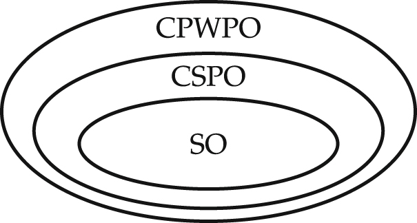
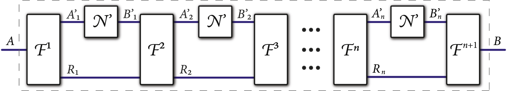
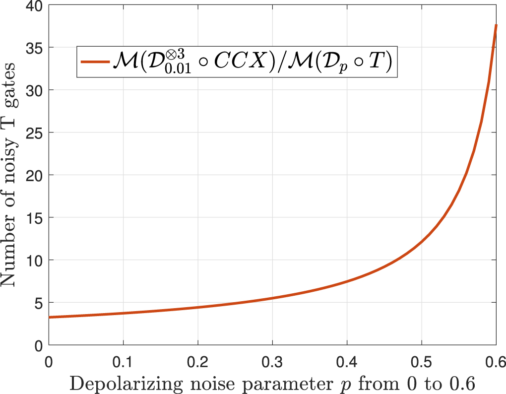
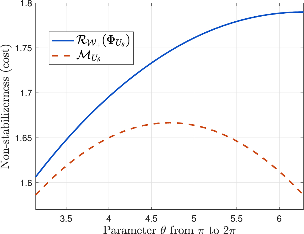
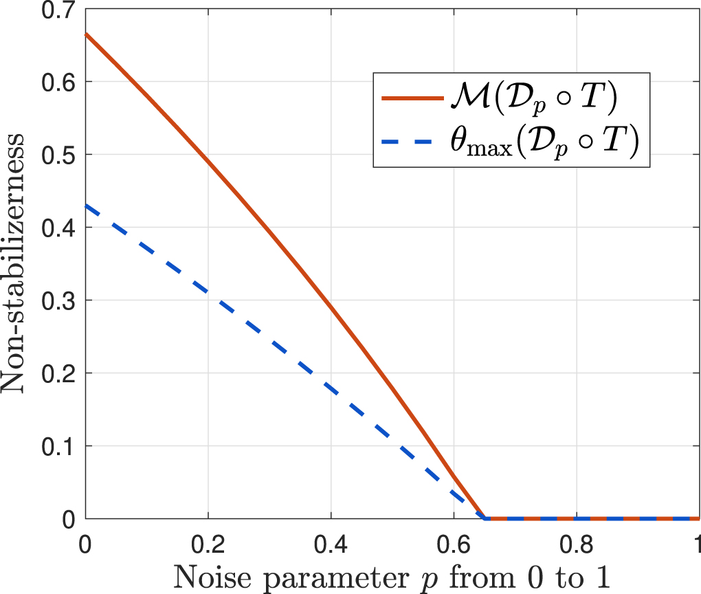