


Abstract
We investigate three fundamental issues in the physics of high-Tc cuprates, from the perspective of a recently proposed comprehensive theory for these materials. (a) Orbital ordering × superconductivity. The first issue is the detailed microscopic mechanism that produces an attractive interaction between holes in high-Tc cuprates. (b) Dispersion relation × pseudogap order parameter. The second issue refers to the existence of a pseudogap order parameter, which would be different from zero all over the pseudogap phase and would vanish elsewhere. (c) Chemical potential × quantum critical point location. The third issue concerns the debate as to whether the quantum critical point, located where the pseudogap transition line T*(x) meets the T = 0 axis is inside the superconducting dome or at its boundary. We obtain clearcut solutions for the three issues.
Export citation and abstract BibTeX RIS

Original content from this work may be used under the terms of the Creative Commons Attribution 4.0 licence. Any further distribution of this work must maintain attribution to the author(s) and the title of the work, journal citation and DOI.
1. Introduction
Three fundamental issues, concerning superconductivity (SC), the pseudogap and their interplay, have attracted the special attention of the community of high-Tc SC in cuprates, recently. In this study, we approach all of them, from the perspective of a recently proposed comprehensive theory for these materials [1–3].
The first issue is about what is the detailed microscopic mechanism that produces an attractive interaction between holes in high-Tc cuprates (hole-doped). The second issue refers to the existence of a pseudogap order parameter, which would be different from zero all over the pseudogap phase but would vanish elsewhere. The third issue concerns the debate as to whether the pseudogap transition line T*(x) meets the T = 0 axis inside the superconducting dome or at its boundary.
As far as the first issue is concerned, we show that a peculiar arrangement of the px
and py
oxygen orbitals of the CuO2-planes makes the mutual magnetic interaction of neighboring holes with the localized copper ions, to produce a net attractive interaction between themselves, which is responsible for the emergence of a superconducting phase in the cuprates. This interaction resembles the Kondo interaction, in the sense that it involves a magnetic interaction between localized and itinerant spins. The crucial difference, however, resides in the fact that in the Kondo system, the itinerant spins are essentially free conduction band electrons, whereas, in the case of cuprates, conversely, the itinerant spins are holes belonging to a sophisticated structure of px
and py
orbitals organized on a bipartite square lattice in a particular way such that the mutual hybridization of neighboring holes with the Cu++ ion  orbital, determines the attractive character of the interaction between holes, resulting from the mutual interaction of such holes with the localized copper spins. This is the root of the interaction responsible for Cooper pair formation and for the onset of SC in cuprates. The mediation of this SC interaction is made by the ferromagnetic fluctuations of the localized copper spins.
With respect to the second issue, a remarkable feature of the physics of cuprates is the presence of the pseudogap phase [4, 5], whose signature is the observation of a double peak, in the density of states, having a considerable depletion of states in between then. We show that in the pseudogap phase an order parameter M(kx , ky ), given by the ground-state expectation value of the exciton creation operator, acquires a nonzero value, thus modifying the energy spectrum (and the dispersion relation) accordingly. We, then, demonstrate the existence of a close relation between the energy spectrum and the density of states, namely, the occurrence of two sharp peaks with a depletion in between which is observed in the latter, is a direct consequence of the d-wave symmetry exhibited by the former. This is produced by a pseudogap order parameter whose k-dependence spontaneously breaks the 90°-rotation symmetry of the oxygen lattices.
As we move from the strange metal to the pseudogap region, in particular, we show that the modification that can be observed in the energy spectrum produces the peak separation observed in the spectral density. This serves, indeed, as an overall pseudogap order parameter for the cuprates. We explicitly calculate the spectral density in the strange metal and pseudogap phases of Bi2212, at different temperatures, and show that our results compare very well with the experimental data.
The third issue concerns the debate about the location of the quantum critical point existing right at the place where the pseudogap transition line T*(x) meets the T = 0 axis. The issue here consists in determining whether this point is located inside the superconducting dome or at its boundary. We approach this question by determining, with the help of our model, the chemical potential along the pseudogap line T*(x) as well as along the Tc(x) line. Then, examining the behavior of the chemical potential along both transition temperature lines in the limit when T → 0, we may find whether they meet or not at this point. In the former case the pseudogap line will reach zero at the dome's boundary, whereas in the latter it will do it inside the superconducting dome. The different cuprate materials exhibit either one or another behavior. We show, for instance, that Hg1201 behaves as the former while Bi2212, as the latter.
One of the nice features of our theory is the fact that it can be tested, namely, we can calculate, out of it, the values of physical observable quantities which can be compared with the experimental data available for several cuprate compounds. Indeed, based on this theory, we have been able to obtain, for instance, analytical expressions for the SC and PG transition temperatures as a function of doping, namely, Tc(x) and T*(x) and the dependence of Tc on an applied pressure Tc(x, P). We provide a sample of our results for these observable quantities in the supplementary material (https://stacks.iop.org/NJP/24/063009/mmedia).
We have also established the pressure independence of the PG temperature T*(x). Furthermore, starting from such theory, we obtained analytical expressions for the resistivity as a function of the temperature ρ(T) in the PG, SM and FL phases and also in the crossover between the last two. Finally, we have derived expressions for the magnetoresistivity in the overdoped regime. All the above mentioned results are in excellent agreement with the experimental data for LSCO, YBCO and the Bi, Hg and Tl families of cuprates [1–3].
2. The genealogy of the effective Hamiltonian
We are going to examine here the genealogy of the Hamiltonian we use in the theory for SC of high-Tc cuprates, which we introduced recently in [1] and subsequently explored in [2, 3]. This will help to build a perspective on the situation of our model and trace its origin back to the first principles.
2.1. The first generation Hamiltonian
There are clearly three main actors playing a central role in the physics of high-Tc cuprates, which unfolds on the stage of the CuO2-planes: the 3d electrons of the Cu++ ions, and the 2px
and 2py
electrons of the O−− ions. Let us call  ,
,  and
and  the creation operators of electrons with spin σ = ↑, ↓ belonging to these orbitals. The electronic density of electrons belonging to orbital a = d, px
, py
is denoted by
the creation operators of electrons with spin σ = ↑, ↓ belonging to these orbitals. The electronic density of electrons belonging to orbital a = d, px
, py
is denoted by  . It is quite plausible that the essential features of the behavior of these electrons should be properly described by the so-called three bands Hubbard model (3BHM) [6–13], which corresponds to the Hamiltonian
where  represents the copper ions lattice positions, R denotes the positions of the oxygen atoms in one sublattice and di
, i = 1, ..., 4 its four nearest neighbors located in the opposite sublattice. This the first generation model.
represents the copper ions lattice positions, R denotes the positions of the oxygen atoms in one sublattice and di
, i = 1, ..., 4 its four nearest neighbors located in the opposite sublattice. This the first generation model.
2.2. The second generation effective Hamiltonian
As we dope the system by the introduction of holes, these become the main actors on the stage of CuO2-planes. Then, a model is required for the description of the physics of the doped holes in such planes. A convenient starting point is a version of the 3BHM that is formulated in terms of holes [11]. This, however, is complicated to such an extent that, in order to extract physical information from it, the model was either approached by numerical methods or by considering simplified versions that could, yet, capture the essential physics.
The simplest example of a model describing the doped holes is the t–J model [14], which assumes that the doped holes form singlet states (Zhang–Rice singlets) with the localized copper spins. Its associated RVB solution [15–17], served as the base for one of the first proposed mechanisms for SC in cuprates [18–20]. It seems, however, that the t–J model does not capture the whole complexity of the high-Tc cuprates.
The spin-fermion (SF) model, which is a natural evolution of the 3BHM [21], offers an appealing framework for the description of the doped holes in cuprates.
The SF-model has been derived by integrating out the electron degrees of freedom in the oxygen orbitals [20, 21], thereby yielding a model that contains just the holes in such oxygen orbitals. These will interact with the localized spins of the copper ions in a Kondo-like way.
The SF Hamiltonian comprises the three terms below [1, 22]: the hopping term, the AF Heisenberg term and the Kondo-like term, namely
where  ,
,  are the hole creation operators on sites R and R + d, respectively, of the A, B oxygen sub-lattices and SI
are the spin operators of the localized Cu++ ions.
are the hole creation operators on sites R and R + d, respectively, of the A, B oxygen sub-lattices and SI
are the spin operators of the localized Cu++ ions.
In the equation above,

which is the spin operator of holes belonging to the px
, py
oxygen orbitals, which are associated, respectively, to the A and B sub-lattices. The sign factors ηA
, ηB
= ±1 originate in the exchange integrals involving the atomic orbitals and are determined by the sign of the half-portion of the px
and py
oxygen orbitals that overlaps with the one-fourth portion of the  copper orbitals, whose sign we denote by either ηC
= ±1 or
copper orbitals, whose sign we denote by either ηC
= ±1 or  .
.
In what follows, we focus on two possible configurations of sign factors  , which are explicitly displayed in the figures below (red and green): figures 3 and 1. These are quantum states with properties determined by the dynamics of oxygen orbitals. The ground-state, in particular can be either of them or a linear combination thereof. It turns out that the ground-state corresponding to the configuration depicted in figure 3, leads, according to equation (15), to an attractive interaction between holes, which will ultimately generate a SC phase. This is an important difference between our model, which is derived from the 3BHM with the orbital phases convention depicted in figure 3, and the usual version of the 3BHM, which is found in the literature, and uses the phases arrangement depicted in figure 1.

Figure 1. The CuO2 planar lattice with sub-lattices A and B represented in green and gray, respectively. This configuration, which corresponds to the base shown in figure 4, leads the magnetic interaction between localized and itinerant spins to produce hole-attractive and hole-repulsive interactions among the itinerant holes.
Download figure:
Standard image High-resolution imageAccording to figures 2 and 3 (red configuration), we see that the oxygen orbitals can arrange themselves in such a way that ηA
ηC
and  have opposite signs for all nearest neighbor (A, B) pairs.

Figure 2. The base of a crystal structure of the oxygen orbitals around the Cu++ ions in the CuO2 planar lattice, which minimizes the energy in the SC phase. This configuration of oxygen orbitals leads the magnetic interaction between localized and itinerant spins to a hole-attractive interaction. The black circles represent Cu ions, whereas the oxygen ions belonging to sub-lattices A and B are represented in red and gray, respectively.
Download figure:
Standard image High-resolution image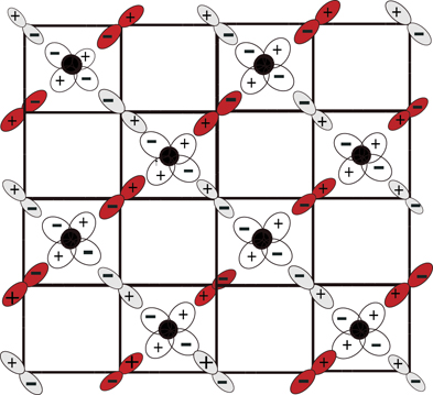
Figure 3. The CuO2 planar lattice with sub-lattices A and B represented in red and gray, respectively. This configuration, which corresponds to the base shown in figure 2, leads the magnetic interaction between localized and itinerant spins to an effective hole-attractive interaction for all nearest neighbor holes and is responsible for the SC in cuprates. Notice that the base depicted in figure 2 consists in a dimerization, if compared with the one in figure 4.
Download figure:
Standard image High-resolution imageThis fact will be crucial for the magnetic interaction existing between the itinerant oxygen holes and the localized copper ions to produce a net attractive interaction between the holes belonging, respectively, to the A and B sub-lattices. At the same time this arrangement of the signs of the oxygen orbitals guarantees the super-exchange coupling that governs the magnetic interaction among the Cu-ion spins to be antiferromagnetic. We can see clearly, therefore, that a close relation exists between the occurrence of a Néel state in the parent compound and the emergence of a superconducting state upon doping. The interaction between the copper and oxygen spins resembles the one found in Kondo systems, in the sense that it couples the spins of itinerant holes with the spins of localized copper ions. Notice, however, the profound difference that exists between the physics of the Kondo effect and that of the high-Tc cuprates: in the first case the itinerant electrons are essentially free, whereas in the present case the holes belong to the px , py oxygen orbitals.
In the case of the cuprates, the holes, rather than being free, belong to a highly organized network of atomic p-orbitals of the oxygen ions. We shall see that there is a peculiar organization of the signs of such oxygen orbitals, that generates an effective attractive interaction between the holes belonging to the two (A, B) oxygen sub-lattices thereby leading to a superconducting state. Below Tc, such arrangement, which leads to a superconductor state is, energetically, most favorable.
Just for completeness, we mention that the t–J model can be obtained from the SF model by means of a perturbative 1/JK approach [14].
2.3. The third generation effective Hamiltonian
The SF Hamiltonian, given by (2), does not include the description of the Coulomb repulsion between the holes. Given the relative magnitude of such interaction, when compared with the magnetic ones (for LSCO Up = 5.5 eV, JAF = 0.43 eV, JK = 1.17 eV [1]), however, it seems quite natural to include Hubbard repulsive terms for the holes in the CuO2 planes. This leads us to a third generation Hamiltonian, namely, the SF-Hubbard model [1, 6], whose Hamiltonian possesses the four terms below:

where the first three terms are given by (2) and  are the hole densities in sub-lattices A, B, respectively.
2.4. The fourth generation effective Hamiltonian
The SF-Hubbard model is the starting point for our proposed theory for the cuprates. In order to derive the effective Hamiltonian we propose for describing the interaction among the doped holes, we are going to perform two operations on the SFH Hamiltonian: (1) we are going to trace over the ferromagnetic fluctuations component of localized spins SI in HAF and HK; (2) we are going to do a perturbation expansion on the hopping term H0 with respect to the unperturbed Hubbard term HU. These two operations will lead to our effective Hamiltonian for the cuprates, which is, therefore, a fourth generation Hamiltonian.
We start by tracing out the ferromagnetic fluctuations of the localized spins [22]. This will produce an effective interaction Hamiltonian, H1[ψ], for the itinerant holes.
We have

By using an appropriate base of coherent spin states, namely {|N⟩}, with the property

(s = 1/2 is the spin quantum number) we can express the trace over such localized spins SI as a functional integral over the classical vector field N of unit length (see, for instance [1]) from which, we have [22]

We now consider separately the antiferromagnetic and ferromagnetic components of N, denoted, respectively, by n and L. We then write, expanding up to the second order in the lattice parameter a

such that |N|2 = |n|2 = 1 and L ⋅ n = 0.
We can re-write the trace over SI as a double functional integral on n and L [1]:

Then, inserting (8) in (7) and expanding in a, we obtain
We are going to integrate out the ferromagnetic fluctuations by performing the quadratic functional integral on L. This will produce three terms: the 2nd term squared, which provides a kinetic term for n [1], the 1st term squared, which produces an effective interaction among the itinerant doped holes (which is the 3rd term in the exponent below) and the crossed term, which vanishes [22, 23]
where  is the spin stiffness and c = JAF
a is the spin-waves velocity.
is the spin stiffness and c = JAF
a is the spin-waves velocity.
Using the fact that the continuum limit involves the replacement a2 ∑k ↔ ∫d2 r, we conclude that
where ZNLσM is the partition function of the nonlinear sigma model (see, for instance [22]).
From the last term in (12) we see that, indeed,

Inserting the expressions for  and
and  in (13), we obtain, up to a constant,
From figure 4 we see that

For this reason, the above interaction is always attractive between nearest neighbor holes, which belong to different sub-lattices.
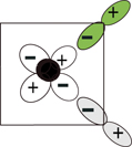
Figure 4. The base of a possible crystal structure of the oxygen orbitals around the Cu++ ions in the CuO2 planar lattice. This configuration of oxygen orbitals leads the magnetic interaction between localized and itinerant spins to a hole-repulsive interaction for some of the nearest neighbor holes and to a hole-attractive interaction to the others. The black circles represent Cu ions, whereas the oxygen ions belonging to sub-lattices A and B are represented in green and gray, respectively.
Download figure:
Standard image High-resolution imageWe conclude that a crucial ingredient of the mechanism that leads to an attractive interactions between neighboring holes in cuprates, being, consequently, responsible for the SC in these materials, is the oxygen p-orbitals organization depicted in figures 2 and 3.
By examining figures 5 and 6, where the oxygen p-orbitals configurations corresponding to the two states introduced in section 2.1 was made more explicit, we immediately conclude that the orbital arrangement depicted in red, which is responsible for the hole attractive interaction that leads to the superconducting phase of cuprates, spontaneously breaks the 90° rotation symmetry. This explains the peculiar symmetry of the SC order parameter in cuprates. This study reveals in a clearcut way the interplay between the symmetry of the SC order parameter and the pairing mechanism itself.
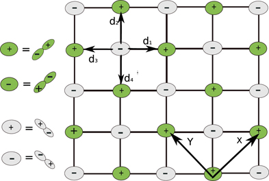
Figure 5. The A and B sub-lattices, represented in green and gray, respectively. The sign of the p-orbitals is explicitly shown, indicating that each orbital of a given sub-lattice has four nearest neighbor orbitals belonging to the other one, indicated by di , i = 1, ..., 4 with an opposite sign.
Download figure:
Standard image High-resolution image
Figure 6. The A and B sub-lattices, represented in red and gray, respectively. The sign of the p-orbitals is explicitly shown, indicating that each orbital of a given sub-lattice has four nearest neighbor orbitals belonging to the other one, indicated by di , i = 1, ..., 4 such that the ones corresponding to i = 1, 3 have the same sign, while those corresponding to i = 2, 4 have a different sign.
Download figure:
Standard image High-resolution imageThe complete effective Hamiltonian we use for describing the cuprates is obtained by carrying on a second order perturbation theory on the H0 + HU terms [1]. Including this result, we obtain the following effective Hamiltonian:
where gS , is the hole-attractive interaction coupling parameter and gP , the hole-repulsive one, given, respectively, by

This is the effective Hamiltonian of our theory for high-Tc cuprates. In the next section, we present it, in the form containing just tri-linear interactions.
3. The effective Hamiltonian
3.1. Hubbard–Stratonovitch fields
We can write our effective Hamiltonian in terms of the Hubbard–Stratonovitch fields Φ and χ, as [1]
In order to describe the doping process, we add to the above Hamiltonian the chemical potential term

where d(x) is a function of the stoichiometric doping parameter x, to be determined self-consistently.
From this we derive the field equations

and

Observe that Φ† creates two holes with opposite spins, each one in the neighboring sites A, B, located, respectively, at (R, R + di ), where
where  and
and  are primitive vectors of the oxygen lattices (see figure 6). It is, therefore, a Cooper pair creation operator. χ†, conversely, creates an electron and a hole with parallel spins, also in such neighboring sites A, B. It is, therefore, an exciton creation operator.
3.2. The SC and PG order parameters
Let us examine the ground-state expectation value of these operators, namely

and

Notice that, because of the invariance under Bravais lattice translations, it follows that Δ(di ) and M(di ) do not depend on the Bravais lattice sites' position R, rather, they depend only on di .
According to figure 6, we see that

and

Now, considering that

and that

we find, using the fact that  ,
,

and also that

where  .
.
We see that the SC and PG order parameters both have a d-wave symmetry, namely, change the sign under a 90° rotation, and have nodal lines along the  and
and  direction.
3.3. The thermodynamic potential
Replacing Φ and χ by their ground-state expectation values Δ and M in the Hamiltonian (18), and using this in the grand-canonical ensemble, after functional integration over the fermionic (holes) degrees of freedom, we obtain the grand-canonical potential

where ZG is the grand-partition function.
The stationary equations obtained by minimizing Ω(Δ, M, μ) with respect to each of its variables leads, respectively, to equations (1), (5) and (9) of the supplementary material, which are our starting point for obtaining the phase diagram of cuprates.

Figure 7. The spectral weight for Bi2212 at T = T* = 190 K, namely, at the boundary between the SM and PG phases (arbitrary units). Experimental data from [5]. Solid line is a plot of (46), in the limit where M → 0. Observe that the distance between the two peaks collapses to zero in this limit.
Download figure:
Standard image High-resolution imageFor the sake of simplicity, in the presentation of the model made so far in the present study, we have considered the case of a single-layered cuprate. The general case of cuprate compounds containing N CuO2 planes intercepting the unit cell has been considered in detail in [1] (see also the supplementary material) and can be easily introduced. The multi-layered character of a cuprate manifests itself through an enhancement of the SC coupling parameter: gS → NgS (N is the number of layers) [1]. Such observation has allowed for an accurate prediction of the optimal SC transition temperatures for the different-N multi-layered compounds of a given family of cuprates (e.g. Bi, Hg, Tl) [1].
4. The density of states and the PG order parameter
4.1. General expression
Consider a system with eigen-energies given by  . The spectral weight, for such a system, is defined as [22]

For a system with a volume V, we have

or, equivalently,

from where we conclude that the spectral weight per unit volume coincides with the density of states g(ω).
Also,

where

4.2. The spectral weight in the strange metal phase
In the SM phase, we have M = 0, and the dispersion relation is given by [1]

where V is proportional to the kinetic hopping parameter t. Expanding around the Brillouin zone center k = 0, we have

Inserting this in (36), and using the result

where θ(x) is the Heaviside function, we obtain the spectral weight in the SM phase:

4.3. The spectral weight in the pseudogap phase
In the PG phase, we have M ≠ 0 and considering just the two oxygen sub-lattices, we have

Now, making an expansion analogous to that we did before, but now expanding around the center of the elliptical Fermi surface pockets, namely,  [1] we obtain

where  , kx
= k cos θ and ky
= k sin θ.
, kx
= k cos θ and ky
= k sin θ.
Considering that the Bessel function J0(x) is given by

and using (36), we arrive, after performing the θ-angular integration, at

Now, integrating over λ [24], we obtain
Finally, integrating on y, we arrive at [24]

where  . This function has sharp peaks at ±A, as we can see in figures 8–11. The peaks occur at frequencies which are determined by the pseudogap order parameter M, being always nonzero for M ≠ 0. The case M → 0, occurs for T → T∗ and is depicted in figure 7.

Figure 8. The spectral weight in the PG phase for Bi2212 at 144 K (arbitrary units). Experimental data from [5]. Solid line is a plot of (46).
Download figure:
Standard image High-resolution image
Figure 9. The spectral weight in the PG phase for Bi2212 at 123 K (arbitrary units). Experimental data from [5]. Solid line is a plot of (46).
Download figure:
Standard image High-resolution image
Figure 10. The spectral weight in the PG phase for Bi2212 at 100 K (arbitrary units). Experimental data from [5]. Solid line is a plot of (46).
Download figure:
Standard image High-resolution image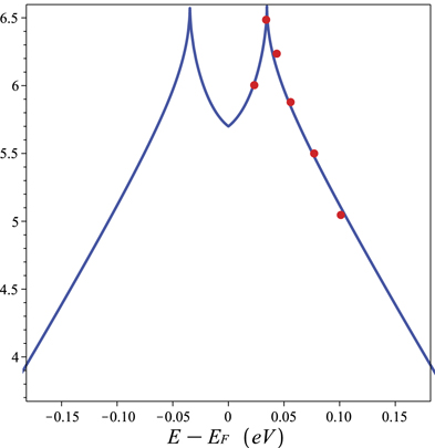
Figure 11. The spectral weight in the PG phase for Bi2212 at 92 K (arbitrary units). Experimental data from [5]. Solid line is a plot of (46).
Download figure:
Standard image High-resolution imageThe opening of a region of lesser spectral weight in between the two peaks has been observed in the whole PG phase by means of tunneling experiments and is a convincing experimental proof of the correctness of our prediction about the existence of a PG order parameter in the whole PG phase of the cuprates: the PG order parameter is proportional to the peaks separation.
We emphasize the fact that the double peak structure, with a depletion in between, appearing in the spectral weight is a direct consequence of the asymmetry of the PG order parameter under 90° rotations. Should we have a homogeneous order parameter M, this would imply a real gap (not a pseudogap!) with the spectral weight vanishing in between [−M, M]. It is remarkable that the same asymmetry of the SC order parameter under 90° rotations is responsible for the pairing of holes, as we showed in section 2.4, equations (15) and (16).
5. The chemical potential
5.1. μ(T) at the SC transition
We may invert equation (1), of the supplementary material and thereby express the chemical potential as a function of the temperature on the Tc(x)-curve, namely
where the last two equations are implicit for the chemical potential μ(T).
5.2. μ(T) at the PG transition
In order to determine the chemical potential right over the PG transition line, we invert the equation (5) of the supplementary material, meant for T* and obtain

where  , which appears in the equation above, is a function of the gP
coupling parameter, appearing in (17), which is defined in the supplementary material.
, which appears in the equation above, is a function of the gP
coupling parameter, appearing in (17), which is defined in the supplementary material.
In figures 12, 13 and 14 we plot the solutions μ(T) along the Tc transition line, both in the underdoped (blue) and overdoped (red) regions, as well as  along the T* transition line (green).

Figure 12. The chemical potential for LSCO along the SC and PG transition curves: Tc(x) (blue—underdoped and red—overdoped) and T*(x) (green).
Download figure:
Standard image High-resolution image
Figure 13. The chemical potential for Bi2212 along the SC and PG transition curves: Tc(x) (blue—underdoped and red—overdoped) and T*(x) (green).
Download figure:
Standard image High-resolution image
Figure 14. The chemical potential for Hg1201 along the SC and PG transition curves: Tc(x) (blue—underdoped and red—overdoped) and T*(x) (green).
Download figure:
Standard image High-resolution imageWe then compare these results with the corresponding figures (figures 15, 16 and 17) for the phase diagram T × x. Segments with a given color correspond to the corresponding segment in the phase diagram graph.
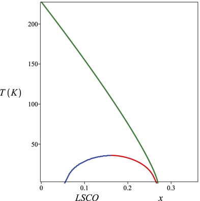
Figure 15. The phase diagrams of LSCO, showing the transition curves Tc(x) and T*(x).
Download figure:
Standard image High-resolution image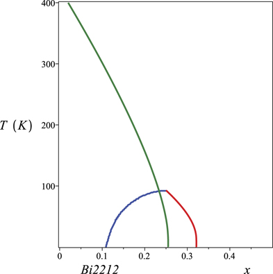
Figure 16. The phase diagrams of Bi2212, showing the transition curves Tc(x) and T*(x).
Download figure:
Standard image High-resolution image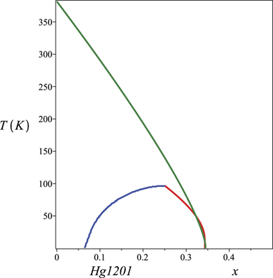
Figure 17. The phase diagrams of Hg1201, showing the transition curves Tc(x) and T*(x).
Download figure:
Standard image High-resolution image
Observe that what determines whether the PG transition curve ends inside the SC dome or not are the values of the chemical potential at T = 0 for the SC and PG curves, namely μ(T = 0) and  . In the examples considered here, such values coincide for LSCO and Hg1201 and differ for Bi2212. This implies a back-bending of the T* line for the latter material, as we can see in figure 16 and has been observed in [5]
6. Conclusion
The study we report here brings forth the complete elucidation of three fundamental issues in the physics of high-Tc cuprate superconductors.
The first one concerns the issue as to what is the ultimate nature of the interaction that makes the holes doped into the oxygen px and py orbitals to form Cooper pairs and, thereby, to exhibit a SC phase.
The second one concerns the existence of a PG order parameter, that would be different from zero in the whole PG phase and zero outside of it, in such a way that it could be used to unequivocally characterize such a phase.
The third one consists in determining whether the quantum critical point located at the end of the pseudogap line T*(x) can be found either inside the SC dome or at its boundary.
We have shown that the interaction that leads to Cooper pair formation derives from the Kondo-like magnetic interaction that exists between the itinerant oxygen holes and the localized copper spins. A crucial issue, however, is the peculiar arrangement of the oxygen p-orbitals depicted in figure 3, which guarantees an attractive interaction for all nearest neighbor holes.
Below Tc, the energetically most favorable configuration of the oxygen p-orbitals, which hybridize with the copper ions d-orbitals is the one represented in red-white, in figures 3 and 6. Notice that this configuration breaks the 90° rotation symmetry and naturally leads to DDW SC and PG order parameters [25–27]. Besides that, remarkably, this orbital arrangement leads to an ever attractive effective interaction between neighboring holes, by means of a mutual magnetic interaction with the closest copper ion.
Observe that, comparing the configurations that repeat themselves, given in figure 2, with the one in figure 4, we conclude that in order to produce the orbital arrangement that will produce the attractive interaction, which leads to SC, the system undergoes a dimerization that resembles the one found in polyacetylene [28]. Furthermore, the dimer configuration exhibits an AF ordering of the copper spins, associated with the super-exchange mechanism.
Secondly, our analysis shows that the spectral density which results from an energy dispersion relation containing a d-wave gap parameter, such as the one in (27), exhibits two sharp peaks, symmetrically placed around the Fermi level at positions proportional to  . In between the two peaks, the density of states is depleted but non-vanishing, that is why it is properly called 'pseudogap'. Should the gap parameter be uniform in k-space, we would have actual gap, with the spectral density vanishing in between the peaks. The peak separation in the spectral density, which is observed along the whole PG region is the PG order parameter. We have seen that it derives directly from the 90° rotation symmetry breakdown that leads to expression (27) for the pseudogap.
We calculate the spectral density corresponding to the dispersion relation in the presence of a d-wave symmetric pseudogap order parameter, given by (37) and (38) and show that it leads to a double-peaked spectral density, such that the peaks, symmetrically placed around the Fermi level delimit a region where the spectral density is depleted. Our theoretical results are in good agreement with the experimental data for Bi2212, as well as with a Ginzburg–Landau approach to competing orders in cuprates [5, 29].
Finally, by determining analytical expressions for the chemical potential along the SC and PG transition lines, we are able to predict whether they coincide or not in the limit T → 0. In the former case the quantum critical point located at T* = 0 is placed at the dome boundary, whereas, in the latter, it will be inside the SC dome. Explicit results are provided for LSCO, Bi2212 and Hg1201 and should be compared to the results in [29].
Acknowledgments
The author is grateful to Nigel Hussey for interesting and stimulating conversations. This study received partial financial support from CNPq, FAPERJ and CAPES.
Data availability statement
The data that support the findings of this study are available upon reasonable request from the authors.