
Abstract
Signal transduction networks are responsible for transferring biochemical signals from the extracellular to the intracellular environment. Understanding the dynamics of these networks helps understand their biological processes. Signals are often delivered in pulses and oscillations. Therefore, understanding the dynamics of these networks under pulsatile and periodic stimuli is useful. One tool to do this is the transfer function. This tutorial outlines the basic theory behind the transfer function approach and walks through some examples of simple signal transduction networks.
Export citation and abstract BibTeX RIS

Original content from this work may be used under the terms of the Creative Commons Attribution 4.0 license. Any further distribution of this work must maintain attribution to the author(s) and the title of the work, journal citation and DOI.
1. Introduction
Signal transduction networks are systems of biomolecules that deliver signals from one point in space to another, such as from the cell surface to the nucleus. This process facilitates biochemical changes in the cell that dictate phenotypic changes, such as cell growth, death, differentiation and migration. Different input patterns on the same network can yield different phenotypic outcomes. As such, there has been much focus on understanding the dynamics of networks in response to different inputs—in particular, pulses and oscillations, which occur physiologically for some hormones. Studying networks under periodic forcing is one way to mimic these systems but also is a general approach to understand system dynamics in any network. In the literature, this is often called the frequency-domain approach (as opposed to the time domain). In the frequency domain with periodic forcing, the response output is at the same frequency as the input but is attenuated in amplitude and shifted in phase. A compact mathematical representation of the ensuing dynamics is called the transfer function. The transfer function method from conventional control theory is a popular and highly useful tool that people employ to study this frequency domain. In this tutorial we espouse the use of a transfer function approach to understanding signal transduction networks. The paper is organised as follows. In sections 1.1 and 1.2 we give experimental and theoretical motivations of why studying biochemical networks in cells under periodic forcing is useful. In section 2 we introduce the reader to the mathematical background. In section 3, we illustrate the mathematical approaches covered in section 2 and apply them to some simple network motifs yielding quantitative results. Section 4 covers a qualitative approach to gleaning the essential features of the transfer function given a network architecture. In section 5, we discuss some of the limitations of the transfer function approach and give an example where the transfer function fails. In section 6 we conclude with some final remarks.
1.1. Experimental motivations
Most cell biology experiments involve using a constant concentration of perturbant (effectively a step-function in time). Yet, in physiological systems, levels of hormones are not constant but can vary in time—often exhibiting rich dynamics (pulsing, fast and slow transients). One way of investigating dynamics in a systematic way is through using pulses or periodic forcing. There are other reasons for using periodic forcing. The number of input parameters can be increased (frequency in addition to amplitude). Periodic forcing in some cases has been reported to entrain an otherwise heterogenous responding system. In many cases the degree to which a system can be entrained by external periodic forcing can be investigated [1].
Especially with advancements in technologies like microfluidics and optogenetics, performing these periodic forcing experiments have become increasingly viable [2, 3].
Studying system dynamics in the frequency domain framework also presents a variety of advantages over its time domain counterpart.
The first area concerns signal processing and biological computing. Frequency domain methods allow extra information to be encapsulated into signals. Non-oscillatory signals lack the 'degrees of freedom' that sinusoidal ones have, such as periods and modulations, into which information can be encoded [4]. The periodic repetition of signals also allow for removal of unwanted information like transient effects and noise. Related to this information encoding is the ability to measure the information carrying capacity or bandwidth [5]. Bandwidth is obtained by measuring pathway activity in response to inputs at varying frequencies. It is a property often neglected in the time domain. Considering signal transduction networks as machinery with bandwidth opens doors towards a computational picture of biology. Like how two networks can differ in information carrying capacity, they can also have different response activities to the same signal. The window of optimal response activity is called the dynamic range. Bandwidth and dynamic range are almost synonymous quantities, and understanding one helps with understanding the other. This is especially seen in signal transduction pathways that consist of multiple components operating on a different timescales [6]. With these specific windows of information capacity and dynamic response, we can see how using the right frequency of input signals in complex biological systems allows us to observe special functionalities of biological systems and probe for the existence of system components [3, 7–13].
The second area concerns biological engineering and medicine. Understanding dynamic ranges also presents avenues into controlling and engineering biological systems. This is especially useful in medicine and drug development—or 'frequency domain medicine'. In embryonic development, initial vertebrae formation is controlled by oscillating levels of gene expression that travel between the two ends of the embryo along a tissue called the presomitic mesoderm. There is a specific frequency, depending on each species, required at this stage for successful vertebrae formation. Frequencies too high or low cause abnormalities in vertebral development. This frequency is determined by the activity of the Notch, Wnt and fibroblast growth factor (FGF) pathways. Controlling these pathways allows us to control embryonic development [14–16]. Another example is the extracellular-regulated-kinase (ERK)/mitogen-activated protein kinase (MAPK) pathway, which is responsible for cell proliferation. ERK pulses can be frequency modulated. Different modulations yield different proliferation rates. Knowing when and how to control frequency modulation in the ERK/MAPK pathway can allow us to control cell growth [7].
1.2. Theoretical motivations
The description of an input signal in terms of periodically varying functions enables any input signal to be described via Fourier analysis. The transfer function approach enables a compact description of network dynamics. As we shall show below, the transfer function approach simplifies the solution of differential equations into a solution of algebraic equations. Transfer functions are modular and can be added following simple mathematical rules to represent large signal transduction networks.
2. Mathematical background
The transfer function approach makes one very basic assumption—that our input–output system can be described by a set of dynamical equations in continuous time. Given this criteria, a sequence of logical consequences follow and give rise to our transfer function.
Dynamical equations in continuous time take the form of differential equations. All differential equations have a linearised form. Linear differential equations in time have an equivalent form in frequency. These frequency-domain equations give us our transfer function.
In this section, we will walk through this logic together—covering the mathematical background along the way. We draw upon the formalisms presented in [17–19].
2.1. Dynamical equations
Physical processes can often be modelled using equations that evolve in time. We call these dynamical equations. For continuous time, dynamical equations take the form of differential equations.
To illustrate this, consider a system
 that evolves in continuous time
  . In the case at hand,
  is our signal transduction network. Suppose that
  can be fully described by a set of variables

That is, at any point in time  , the state of
  is defined by the set of values

For signal transduction networks, each  might represent the quantity of a different biochemical species present in the network. These
  terms are called state variables. The column vector of all state variables forms the state vector

Let us further suppose that we can interact with the system, such as by pipetting in and out species. That is,  accepts inputs from and returns outputs to the external environment. Denote the set of inputs as

and outputs as

The respective input and output vectors are

Since the system is fully described by its state variables, the time evolution of  is equivalent to the time evolution of
  .
.
If each  can be described by an ordinary differential equation relating its first time derivative to a function of the set of state and input variables, namely

then we have all the dynamical information about the system required to describe its time evolution packaged into a set of  equations. That is, the time evolution of
  is captured in the set of ordinary differential equations

This can be expressed in vector form as

where

Similarly, if each output variable can be expressed in terms of the state and input variables, then the dynamical information for the outputs are packaged into the following set of  equations

or alternatively in vector form

where

Together equations (8) and (11), or equivalently (9) and (12), make up what is known as the state space representation of a dynamical system. They are also individually referred to as the state equation and state observation equation, respectively. With the right choice of elements in sets  and
and  , one can always describe a continuous time dynamical system by equations (8) and (11); or equivalently (9) and (12). As a simple example, consider the dynamical equation

and output equation

With the following choice of state variables

and, consequently, output variable

we can express our original equations in forms (8) and (11) as follows:


2.2. Equilibria
A system may have one or more special combinations of values of state and input variables such that its state remains stationary in time. That is, there may exist specific sets of  and
and  for which, once the system assumes, prevent
  from changing at future times. Such special sets of values, when substituted into equation (8), reduce each row to zero:

telling us that the rate of change of each state variable is zero.
Each of these special sets of values defines a special coordinate

in parameter space. These special coordinates are termed equilibrium coordinates, or simply equilibria.
2.3. Linearised dynamical equations
We wish to arrive at the transfer function from our state space formulation. However, there is a problem—equations (8) and (11) can be nonlinear. Nonlinear equations do not (strictly) have transfer functions. Only linear equations have transfer functions. A nonlinear equation may, however, have local regions where it behaves approximately linear. In these regions, an approximate transfer function can be obtained. In this sense, the closest equivalent to the transfer function of a nonlinear equation is the transfer function of its local linear equations.
To obtain these local linear equations, we must linearise their original nonlinear forms about their equilibria. Linearisation involves approximating a function with its first order Taylor polynomial about a point of interest. The first order Taylor approximation of a function  about coordinate
  is:
is:

Equivalently, we can recentre the function by defining  and say:

If we choose a  coordinate such that
  , then equation 22b
reduces to
, then equation 22b
reduces to

That is, for these special coordinates, the recentred approximation  is equal to the original approximation
  .
.
If the function we are trying to linearise were to be any of the dynamical equations in equation (8), that is  , then these special
  coordinates would just be the equilibria that we mentioned in section 2.2. We can see this more explicitly if we try to Taylor approximate
  about arbitrary coordinate
  :
:

Now, if  , then

But, as we have established in equation (20),  . Therefore, equation (24) reduces to the form of equation (22c
):
. Therefore, equation (24) reduces to the form of equation (22c
):

Approximating the dynamical equations in (8) and (11) by their first order Taylor polynomials about arbitrary equilibrium coordinate

gives

and

respectively, where  and
and  . The corresponding matrix form of these two linearised systems of equations are

and

where  ,
,  ,
,  and
and  are derivative matrices defined by entries at row
  and column
  :
:


So, given a system near equilibrium, we can approximate its dynamics from equations (9) and (12) with the simpler versions in equations (29) and (30).
If the entries in these derivative matrices are time independent, then equations (29) and (30) reduce to

and

One might imagine the time-dependent matrices  ,
,  ,
,  and
and  to represent time varying rate constants of a signal transduction network, while their time-independent counterparts
  ,
,  ,
,  and
and  to represent fixed rate constants.
2.4. The transfer function
The transfer function is an equivalent representation to the state space representation in equations (32) and (33). It is to the frequency domain what the state space representation is to the time domain. The transfer function describes how a system amplitude modulates and phase shifts incoming sinusoids as a function of frequency.
In terms of cell signalling networks, transfer functions tell us how sinusoidal biochemical inputs are amplified and delayed in the process of turning into outputs (see figure 1).

Figure 1. System receives green oscillatory input and returns red oscillatory output (top). The output is modulated in space by factor  and shifted in time by phase angle
  (bottom). Both waves have identical frequency
  .
.
Download figure:
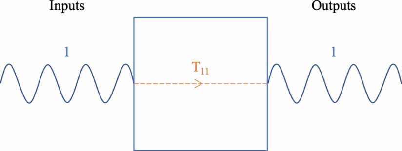
Standard image High-resolution imageFor each pair of inputs and outputs in a system, there is an associated transfer function. That transfer function describes the contribution of that input to its associated output. For a system of one input and one output, a single transfer function exists, see figure 2.

Figure 2. A single-input single-output system has one transfer function.
Download figure:
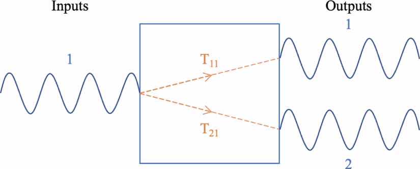
Standard image High-resolution imageFor a system of one input and two outputs, two transfer functions exist: one for the contribution of input 1 to output 1 ( ), another for that of input 1 to output 2 (
 ), as depicted in figure 3.

Figure 3. A single-input dual-output system has two transfer functions.
Download figure:
Standard image High-resolution imageWhen multiple transfer functions exist, they are often written in matrix form with output indices along the rows and input indices along the column. The matrix for figure 3 would be

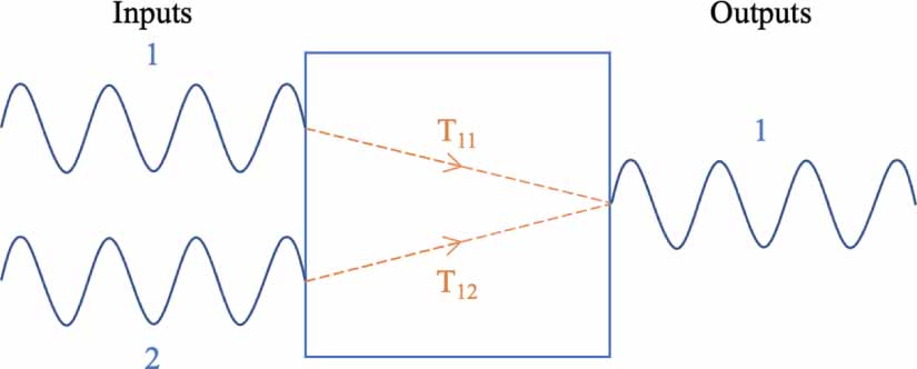
For a system of two inputs and one output, two transfer functions also exist, as shown in figure 4. However, this time, one for the contribution of input 1 to output 1  and the other for that of input 2 to output 1
  .
.

Figure 4. A dual-input single-output system also has two transfer functions.
Download figure:
Standard image High-resolution imageThe associated transfer function matrix now looks like

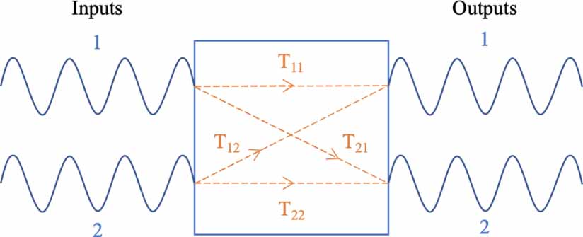
Following the same logic, if we have a two-input to two-output system (as in figure 5), there are now four transferfunctions,

Figure 5. A dual-input dual-output system has four transfer functions.
Download figure:
Standard image High-resolution imagewith associated transfer function matrix

For an arbitrary system with  inputs and
  outputs, there are a total of
  transfer functions, described by the matrix

2.5. Laplace transform
State space representations can be converted into transfer functions. To do this, we will need to employ a mathematical tool called the Laplace transform. For a piecewise continuous function  defined for all non-negative real values of
  , the Laplace transform
  is defined as:

for all complex numbers  such that the integral exists and by analytic continuation where it does not. If
  were to represent time, as is often the case, then
  would represent complex temporal frequency.
  if often shorthanded to
  .
.
2.6. From state space to transfer function
Given a state and state observation equation pair, of form (32) and (33), we can obtain its corresponding transfer function matrix  as follows

where  is the identity matrix and
  is the complex frequency. The derivation for this employs the Laplace transform and some algebra as follows. Starting with equations (32) and (33)

we apply the Laplace transform to each equation to obtain their frequency domain equivalents

Rearranging equation (40a ) gives

Substituting equation (41) into equation (40b ) returns

The transfer function  is formally defined as the ratio of the Laplace transformed output to the Laplace transformed input—that is,
  . Rearranging equation (42) into this form gives the expression we wanted in equation (39)

This matrix has the  structure of that in equation (37).
Equation (39) is often the most systematic way to compute a transfer function from a given state space model. However, it may not be the most efficient or physically meaningful way to obtain a transfer function from a set of dynamical equations that is not yet in state space form. Although we have established that all systems of ordinary differential equations can be expressed in the state space forms (32) and (33), with appropriate choice of state and output variables, the process of doing so sometimes requires tricky changes in variables that have no obvious physical meanings to the original system of interest. This may detract physical insight from the result and turn the calculation into a purely computational exercise with no contextual insight into the biological system. Such is especially the case if derivatives of inputs are present in the dynamical equations. For example, the presence of  here
here

In these cases, it may be more fruitful to first combine the equations (without employing changes of state variables) such that only terms containing the input, output and their derivatives remain. Then performing a Laplace transform and transposing the resulting equation to obtain the ratio of the Laplace transformed output to the Laplace transformed input will return the transfer function. Equivalently, one can start by Laplace transforming the individual differential equations and then combining them to get this transfer function ratio. The preference for order of these steps will depend on the system of equations at hand. We will see an example of this later in section 3.4. It is important to note that we have not done any new math here. All these steps of manual algebraic manipulation and Laplace transformation were already built into the machinery of equation (39), except this machinery was designed in such a way that required a very specific structure of input (i.e. the matrices in equations (32) and (33)) that are not convenient for certain dynamical equations.
2.7. Angular frequency-response functions
Let  , where
  and
and  are real numbers. In the special case of
  , that is for purely imaginary complex frequencies, we obtain the function
  . This is commonly referred to as the (angular) frequency-response function and provides two useful pieces of information: the magnitude frequency-response function
  and the phase frequency-response function
  . Functions
  and
and  are defined as follows


where  and
and  denote real and imaginary components. The plots of
  and
and  against
  are commonly referred to as the Bode magnitude plot and Bode phase plot, respectively.
2.8. Modulatory of transfer functions
Transfer functions are modular. We can obtain new transfer functions from combinations of smaller transfer functions arranged in special architectures. These architectures are called block diagrams and the rules of combining them are called block diagram algebra. Most conventional control theory texts will have an extensive list of block diagram algebra rules. Here, we highlight three rules that we believe will serve the reader well in constructing most signal transduction networks.
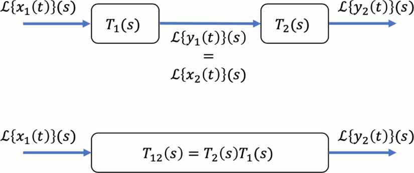
The first is the series rule, which combines two transfer functions in series via a product (see figure 6 for schematic representation):


Figure 6. The series rule converts the top block diagram into the equivalent bottom one.
Download figure:
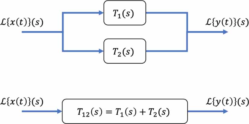
Standard image High-resolution imageThe second is the parallel rule, which combines two transfer functions in parallel (figure 7) via a sum:


Figure 7. The parallel rule converts the top block diagram into the equivalent bottom one.
Download figure:
Standard image High-resolution imageThe last is the closed loop rule (figure 8), which combines two transfer functions in a closed loop via a ratio:


Figure 8. The closed loop rule converts the top block diagram into the equivalent bottom one.
Download figure:
Standard image High-resolution image3. Quantitative examples
To get a better grasp of the ideas in section 2, let us apply it to some simple examples.
3.1. Simple regulation (linear)
Consider the following network (figure 9) in which an input  produces an output
  at constant rate
  while
while  degrades at constant rate
  . This is sometimes referred to as simple regulation under mass action in the literature.

Figure 9. Schematic of simple regulation under mass action.
Download figure:
Standard image High-resolution imageSuppose the dynamics of this process can be described by the differential equation

and output equation

Since this system is already linear, no linearisation is necessary. From our earlier notation, we can say

and

The corresponding derivative matrices are:


Employing equation (39), we obtain the transfer function

This has real and imaginary components

and so, from equations (44a ) and (44b ), the corresponding frequency response functions are

Plotting  and
and  for specific parameter values will give us a better sense of how the network amplitude modulates and phase shifts inputs into outputs.
We can observe two frequency windows of dominant behaviour—one below  and the other above
  . In the former,
  is maximally constant and
  is close to zero. This means inputs are passed with maximal amplitude modulation and relatively little phase shift. In the latter,
  rolls off and
  tends towards
  . Conversely, here, signals are significantly dampened and phase shifted. This behaviour is indicative of a low pass filter with cutoff frequency
  .
.
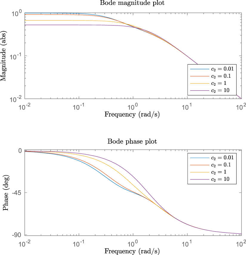
We can also see how  and
and  affect the frequency response of the system, as shown in figure 10. For Bode magnitude plots,
  translates curves vertically while
  translates curves horizontally. For Bode phase plots only
  transforms the curves—translating them horizontally. This means the production rate increases the gain and the degradation rate increases the cut-off frequency.

Figure 10. Bode plots for different  and
and  values. The blue and yellow curves, and orange and purple curves overlap in the Bode phase plot. Plots represent the frequency response of simple regulation model (see figure 9).
Download figure:
Standard image High-resolution image3.2. Simple regulation (nonlinear)
Let us consider the same network (figure 9) except, this time, the production rate is nonlinear. Suppose the state and state observation equations are now

and

Again, from our earlier notation, we can write

and

If we consider the system about some equilibria  , then corresponding derivative matrices are:


Realising that the entries in  and
and  are just constants, we can rename them as follows


But this simply returns the same case as our first example in equation (52), that is


giving us the same transfer function form and Bode plots as previous in equation (53). Here, we can see that the effect of taking a transfer function of nonlinear simple regulation returns that of linear simple regulation. There is one key difference however— cannot be changed independently, rather it must be varied via
  via equation (61). This may restrict the values that
  can assume depending on the values that
  can take.
3.3. Reversible reaction
Consider a slightly more complex architecture (figure 11) in which an input  produces a species
  which in turn produces another species
  such that it reproduces
  again. Let us further allow
  and
and  to degrade. This is an externally driven reversible reaction with degradation under mass action.

Figure 11. Reversible reaction between two degrading species driven by an external input.
Download figure:
Standard image High-resolution imageSuppose the dynamics of this process can be described by the set of linear differential equations


and output equation

Our  and
and  expressions are therefore


and

The corresponding derivative matrices are:

Employing equation (39), we can obtain transfer function

This is the transfer function from input  to output
  . Following the same method as before (see also section 2.7), we obtain the following Bode plots, as shown in figures 12–16. Since we have a handful of parameters, let set each one to unity and take turns varying each to see their effect on the Bode plots.

Figure 12. Effect of varying  .
.
Download figure:
Standard image High-resolution image
Figure 13. Effect of varying  .
.
Download figure:
Standard image High-resolution image
Figure 14. Effect of varying  .
.
Download figure:
Standard image High-resolution image
Figure 15. Effect of varying  .
.
Download figure:
Standard image High-resolution image
Figure 16. Effect of varying  .
.
Download figure:
Standard image High-resolution imageBy varying each parameter from a nominal value, in this case  , we can see how sensitive the frequency response functions are to changes in each parameter. Figure 12, in which the Bode magnitude curves are significantly translated while the Bode phase plots remain invariant, provides a perfect example of how the transfer function gives insight into sensitive or robust parameters that can be manipulated to control with a system.
3.4. Negative feedback loop
Consider the following set of dynamical equations with input  and output
  :
:

This is a special model of a negative feedback loop called the Goodwin model [20]. A schematic of this model is in figure 17. As we mentioned at the end of section 2.6, the dynamical equations have included in them the derivative of the input. We will therefore take the manual route of computing the transfer function.

Figure 17. Negative feedback loop with three species from equation (71).
Download figure:
Standard image High-resolution imageLet us start by linearising our equations about an equilibrium point  . This returns

where  ,
,  and
and  . We wish to obtain an equation for the Laplace transform of our output
  in terms of the Laplace transform of our input
  . This requires us to eliminate
  and its derivative. We begin by combining the first two equations—differentiating equation (72b
)
and its derivative. We begin by combining the first two equations—differentiating equation (72b
)

and then substituting in equation (72a )

Our system of equations is now

Recall that the Laplace transform turns differential equations into algebraic equations. This will greatly simplify our next steps. Transforming both equations gives

Rearranging equation (76a
) for 

and then substituting into equation (76b
) gives the equation for  in terms of
  that we wanted

The transfer function is therefore

A Bode plot of this transfer function for the Goodwin model is shown in figure 18. As expected of negative feedback, bandpass filtering behaviour is observed.

Figure 18. Bode plots for transfer function of the Goodwin model for parameter values: 
 .
.
Download figure:
Standard image High-resolution image4. Qualitative examples
4.1. Ras-Erk MAPK cascade
The example in figure 19 aims to highlight the qualitative predictive power of the transfer function approach. The Ras-Erk MAPK cascade is a low-pass filtering system [21]. It consists of four biochemical species, starting with Ras and ending with Erk (see left hand panel of figure 19). In the experiments described in [21], Ras is activated optogenetically by an external light source. This allows Ras and, hence, the Ras-Erk cascade to be externally driven. By measuring the gain of Erk (output) with respect to light-activated SOS (input) at different input frequencies, the modulation frequency response shown in the right hand panel of figure 19, was observed.

Figure 19. Ontogenetically stimulated Ras-ERK MAPK cascade network (left) and its measured amplitude modulation (right). Adapted from [21] with Copyright © 2013 Elsevier Inc. All rights reserved.
Download figure:
Standard image High-resolution imageSuppose we do not know anything about the rate constants of this system. Let us try to see if we can deduce a plausible functional form of the transfer function corresponding to this network architecture which can recreate the amplitude modulation plot.
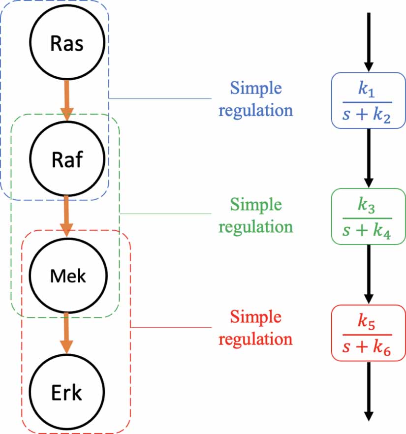
Qualitatively inspecting the cascade architecture, we can identify sequences of simple regulation-like steps (see figure 20).

Figure 20. Identifying the simple regulation components of a sequential signalling cascade.
Download figure:
Standard image High-resolution imageFrom equation (53), each of these steps in figure 20 corresponds to a transfer function of the form

Replacing each node-to-node step in the chain with a transfer function block gives the right-most cascade of transfer functions (see figure 20). Employing the series rule in equation (45), we obtain the following transfer function:

Choosing an arbitrary set of parameters:  , we obtain the following plot in figure 21, which qualitatively matches the blue experimental low pass trend in figure 19. In addition, this gave us a possible phase response curve (figure 21, lower panel).

Figure 21. Bode plots for transfer function of a sequential signalling cascade showing low pass filtering properties.
Download figure:
Standard image High-resolution imageAgain, we stress that this example serves to illustrate qualitative predictions and not reproduce the quantitative result.
4.2. p53-mdm2-ATM feedback loop
This example aims to highlight again the qualitative predictive power of the transfer function approach. The p53-mdm2-ATM feedback loop is involved in cell response to DNA damage. By subjecting cells to noisy DNA-damaging radiation (input) and working out the power spectra of the consequent p53 expression levels (output), the magnitude frequency-response curve for p53-mdm2-ATM was observed [22].
Again, suppose we do not know anything about the rate constants of this system. Let us see if we can deduce a plausible functional form for the transfer function of this network architecture that can recreate the amplitude modulation plot in the solid red curve on the right of figure 22.

Figure 22. p53-mdm2-ATM feedback loop (left) and a model of its amplitude modulation (red solid curve at right). Adapted with permission from [22].
Download figure:
Standard image High-resolution imageBy inspection of the network depicted in figure 22, we can see that each branch of the network resembles a simple regulation system. We can further identify two negative feedback loops—the outer loop between ATM and p53 in figure 23(a), and the inner loop between p53 and mdm2 in figure 23(b). Each loop resembles an interaction between a forward simple regulation step and a backwards simple regulation step. There is a common species in between the two loops—p53. If we suppose the output of p53 is shared by both ATM and mdm2 as inputs, then we can further suppose the transfer function for both of these are the same—as illustrated in green. Flipping the block diagram in figure 23(b) horizontally so that its inputs and outputs align with that of the feedback branch in the block diagram in figure 23(a), we can nest them together into the double closed loop structure as shown in figure 23(c).

Figure 23. Identifying a plausible block diagram for the double nested feedback loop. (a) Identifying the top loop. (b) Identifying the bottom loop. (c) Nesting the loops together.
Download figure:
Standard image High-resolution imageApplying the closed loop rule in equation (47) to the inner most loop in figure 23(c) gives

The block diagram is now reduced to the following single loop as depicted in figure 24.

Figure 24. Block diagram after applying closed loop rule to inner loop.
Download figure:
Standard image High-resolution imageApplying the rule again to this remaining loop gives the transfer function of the entire system

Choosing an arbitrary set of values for the numerators  and denominators
  , we obtain the following Bode magnitude plot in figure 25, which qualitatively matches the form of the solid red curve in figure 22.

Figure 25. Bode plots for transfer function of double nested feedback loop.
Download figure:
Standard image High-resolution image5. Limitations
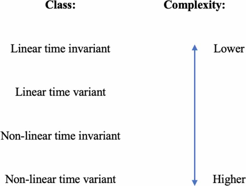
Our discussion up until now has focussed on a class of dynamical systems known as linear time invariant systems. Systems that can be described by the state space equations in equations (32) and (33) are linear time invariant. These systems form the least complex class out of the four classes of dynamical systems (see figure 26).

Figure 26. The classes of dynamical systems and their complexities.
Download figure:
Standard image High-resolution imageThe transfer function method strictly only applies to linear time invariant systems. As we move into the more complex systems, the method breaks down. Let us discuss some shortcomings to the method.
5.1. Superposition
Linear time invariant systems obey superposition. That is, the output of a sum is equivalent to the sum of the individual outputs. Recall from harmonic analysis that all waveforms can be constructed from sinusoidal waves. Since the transfer function tells us how sinusoidal inputs are converted into outputs, it is a tool to predict outputs due to arbitrary periodic inputs in linear time invariant systems (see figure 27).

Figure 27. Predicting the output of a non-sinusoidal periodic input using the transfer function.
Download figure:
Standard image High-resolution imageFor linear time variant, non-linear time invariant and non-linear time variant systems, superposition does not apply. Therefore, the transfer function cannot be used to predict outputs to arbitrary periodic waveforms in these more complex systems.
5.2. Linearisation windows
Recall that, to obtain the local transfer function of a nonlinear function, linearisation was necessary. Often, a linear approximation will only be valid within a limited window about the linearisation point. Therefore, the validity of the associated transfer function will also only be within this window. Let us illustrate this with an example of a saturating system—a common phenomenon in biology (see figures 28–30) .

Figure 28. Saturation curve (blue) and its linear approximation (orange) about the inflection point  .
.
Download figure:
Standard image High-resolution image
Figure 29. The same saturation curve and its Taylor approximation, but now recentred.
Download figure:
Standard image High-resolution image
Figure 30. By visual inspection, sinusoidal inputs of sufficiently small amplitudes should be transformed without clipping (a) whereas those that are too large in amplitude should be clipped (b). This is not reflected in the transfer function of equation (87), however.
Download figure:
Standard image High-resolution imageSuppose our system receives sinusoidal input  about a mean
  . Taking the first order Taylor polynomial about
  gives
gives

This is a reasonable approximation within the window  . Changing variables


gives the recentred curve

Applying the Laplace transform to equation (86) and rearranging to find  gives the transfer function

Its frequency response functions are

and

Equations (88a
) and (88b
) are independent of input amplitude and, so, tell us that the modulation is constant and phase shift is zero for all input amplitudes. The former cannot be the case as inputs larger than the  window should be clipped due to the saturation.
One approach that addresses this shortcoming is the describing function. The describing function can be thought of as a generalised transfer function for nonlinear systems. The describing function  is defined as the ratio of the fundamental component of the output
  to its sinusoidal input
  [23]. In equation form, this is

where  and
and  are the Fourier coefficients of the fundamental component of the output


Saturation can be approximately described by the following piecewise output function

Evaluating the coefficients gives


Substituting equations (92a ) and (92b ) back into equation (89) gives our describing function

The corresponding magnitude and phase frequency response functions are

and

respectively. We can immediately see more information in these frequency response expressions compared to that of the transfer function case in equations (88a
) and (88b
). Plotting  against the ratio of saturation to input amplitude
  returns the following curve in figure 31.

Figure 31. Modulation frequency response of saturation  as a function of the ratio of saturation to input amplitude
  .
.
Download figure:
Standard image High-resolution image
For input amplitudes much greater than the saturation threshold, that is when  is small, the modulation tends towards zero. This is reflects the clipping phenomena of large inputs. As input amplitudes approach the saturation threshold, that is when
  tends towards 1, the modulation approaches
  —the gain of the linear region. This is expected as no clipping occurs in this regime. The latter result is what we previously obtained from the transfer function method in equation (88a
).
—the gain of the linear region. This is expected as no clipping occurs in this regime. The latter result is what we previously obtained from the transfer function method in equation (88a
).
The phase frequency response  here in equation (94b
) is identical to that of the transfer function in equation (88b
), except now we can say it also applies to signals of amplitudes greater than linear window.
here in equation (94b
) is identical to that of the transfer function in equation (88b
), except now we can say it also applies to signals of amplitudes greater than linear window.
6. Conclusion
The transfer function provides an powerful predictive tool into understanding the dynamics of signal transduction networks. Here, we have outlined the theory for the approach and applied it to some simple examples of signal transduction networks to illustrate how it can be used to study signal transduction networks of various architectures, both quantitatively and qualitatively.
Acknowledgments
Nguyen H N Tran acknowledges the receipt of a Swinburne University Postgraduate Research Award scholarship. The authors have declared that no conflicting interests exist.
Data availability statement
The data that support the findings of this study are available upon reasonable request from the authors.