

Abstract
Differential sampling relative to a Josephson waveform, the ac quantum voltmeter (ac-QVM), has been established as the most accurate method for measuring signals below 1 kHz with an uncertainty of 1 part in 108 (k = 1) for 1 V at 250 Hz. Commercial ac-QVMs provide accuracies of about 1 part in 106 up to frequencies of 2 kHz. Here we present a new sub-sampling technique to extend the frequency range of an ac-QVM up to 100 kHz. The measurement results at 1 V RMS amplitude agree well within 5 µV V−1 (k = 1) with the nominal voltage values for all frequencies from 500 Hz to 100 kHz. Two different analogue-to-digital converters are compared, sampling techniques, error sources and corrections as well as detailed uncertainty estimations are discussed.
Export citation and abstract BibTeX RIS

Content from this work may be used under the terms of the Creative Commons Attribution 4.0 licence. Any further distribution of this work must maintain attribution to the author(s) and the title of the work, journal citation and DOI.
1. Introduction
In 2006 quantum based differential sampling measurements for voltage were introduced [1]. Since then the ac quantum voltmeter (ac-QVM) has been further investigated towards higher voltages and frequencies [2–5] also by combining a fast sampler and a programmable Josephson voltage standard (PJVS) [6]. Nowadays, such ac-QVMs have become commercial quantum-based ac voltage standard measurement systems that provide accuracies of about 1 µV V−1 up to frequencies of 2 kHz within minutes of measurement time [6] and are routinely operated at commercial calibration laboratories [7]. However, ac-QVMs are still the subject of investigations for different configurations [8], for Josephson comparisons [9], and especially onsite state of the art comparisons [10]. The full potential of the PTB ac-QVM (one part in 108 at 250 Hz) was demonstrated in a direct comparison with a 1 V pulse-driven Josephson system [11].
As the frequency limit of the differential sampling technique is set by the combination of the transients of the PJVS, the maximum frequency of the PJVS waveform and the limitations of the sampler (bandwidth, input filter, slew rate, etc), a new coherent sub-sampling method has been proposed [12] to extend the frequency range for quantum-based sampling into the 100 kHz range. A frequency range extension of the ac-QVM up to 100 kHz and beyond would be beneficial for many ac calibrations and could provide an independent method for investigating pulse-driven Josephson systems at high frequencies with sub-µV V−1 uncertainties [13]. This is a 50-fold bandwidth extension for present commercial ac-QVMs [7] and would offer a significant increase in productivity compared to conventional ac-dc transfer measurements, which require about one hour to achieve an uncertainty in the range of parts in 106 above 50 kHz.
In this paper, we present the first promising results of an ac-QVM for frequencies up to 100 kHz. Such an increase of measurement bandwidth is possible due to a new coherent sub-sampling technique [12, 14] which has been developed further. Only minor modifications must be applied to the hardware of existing quantum voltmeters which are explained in section 2. The main challenges for sub-sampling towards higher frequencies are the analogue-to-digital converter (ADC) filter and the cable corrections. In section 2 we also report how we have tackled these challenges and how we verified our methods. Measurement results for various parameter settings are presented in section 3. The uncertainty budget in section 4 supports the performance of the new sub-sampling method. Finally, the robustness of this uncertainty budget is supported by further experiments.
2. Setup and methods
2.1. The ac-QVM
Here we briefly summarize the setup, shown in figure 1, which has minor deviations from the one described in [6]. In order to measure the output waveform of the calibrator, a waveform constructed with quantized steps from the PJVS is synchronized to it and their difference is sampled with an ADC. An optically isolated 10 MHz clock from the PJVS bias source acts as a reference for the phase lock input of the calibrator and for a dual synthesizer that provides the clock and trigger for the sampler. The waveform under test from a Fluke 5700A calibrator 1 is reconstructed from measured differences and their associated Josephson voltage steps, so the trigger signal guarantees that the samples from the ADC start at the right phase angle of the PJVS waveform. The RMS value of this reconstructed waveform is then calculated. As described in [6], the number of PJVS samples is a compromise between the frequency being measured, the maximum permissible voltage difference at the input of the sampler, and the settling time around each transition between quantized voltage levels, with two dominant contributions from the sampler and the PJVS.

Figure 1. Measurement setup and synchronization scheme for the ac-QVM in the sub-sampling mode.
Download figure:
Standard image High-resolution imageThe ac-QVM uses commercially available bias sources from NPL 1 [15] or Active Technologies 1 [16] to drive a programmable 2 V array with 16384 (8192 double-stacked) Josephson junctions with a critical current of 3.2 mA and is operated at 70 GHz [17]. The bias system is electrically isolated, and the computer is connected either via an optical ring [18] or an isolated USB. Each of the 14 segments in the binary divided Josephson array is driven by a separate channel of the bias source. The channels have an amplitude resolution of 14 or 16 bits, respectively, and the transitions at the output of the array have risetimes below 200 ns. Faster transients can be achieved with the method described in [19] but this was not employed for the sub-sampling technique.
The system uses a programmable 70 GHz microwave synthesizer [20]. The microwave power is adjusted for equal widths of the zero and first voltage steps. The margins are wider than 1.5 mA, which means that after setting the array bias currents, we usually can run the system for weeks without re-adjusting the parameter settings. No parameter changes were required within the duration of the measurements presented in this paper.
In the direct differential sampling technique [1, 2] the waveform being measured is sampled differentially relative to a Josephson stepwise approximated copy and reconstructed in software from the measured voltage differences. The frequency limit of this technique is set either by the transients of the PJVS, the frequency limit of the PJVS waveform or the limitations of the sampler (bandwidth, input filter, slew rate, etc). Using 20 Josephson steps per period to measure an AC voltage, the transients of the PJVS set an upper limit of 500 kHz. However, the main limitation is usually set by the sampler. Even when using a high sample rate, e.g. 10 MSa s−1 using an NI PXI 5922 1 with a 48-tap 'standard' digital filter, at least 30 data points around each transient must be deleted to avoid undesirable artifacts [6]. The maximum frequency of the ac-QVM is therefore limited to about 10 kHz for 20 Josephson steps per period and to 40 kHz when using just 4 Josephson steps per period.
One approach to increase this maximum frequency is to use the sub-sampling technique [12], described in the following section.
2.2. Sub-sampling technique
We have implemented such a differential sub-sampling method referenced to a low frequency PJVS waveform, one of the methods introduced in [12] and show the signal at the input of the sampler schematically in figure 2. A high frequency sine wave, e.g. fmeas = 100 × fPJVS, is combined with a 40-step PJVS triangular wave at fPJVS. We used a triangular waveform from the PJVS to achieve an even amplitude distribution of the measured differences. The shape of the PJVS waveform is clearly visible in the difference signal at the input of the sampler, shown in figure 2(a). As the PJVS level changes, all phase angles and the complete period of the fmeas waveform being measured is scanned. Figure 2(b) shows the initial part of (a) with the changes in PJVS values marked by the dashed vertical lines. The resulting discontinuities in the waveform at the input of the ADC are also visible. In order to restrict non-linearity effects from the sampler, we only use data points within a certain voltage limit for the reconstruction of the sine wave. As an example, for a 1 V sine wave, a large frequency ratio, e.g. fmeas/fPJVS = 100, and 40 PJVS steps, a voltage limit of 0.071 V is enough to completely cover the gaps between two Josephson steps (1.4142 V/10/2). This voltage limit is marked in cyan/blue in figure 2. White boxes with blue frames indicate the transient times in which measurement data are deleted. We deleted at least 400 data points for the low frequency fPJVS, 20 Hz or 62.5 Hz, to ensure no effect from the PJVS transients. As in the case of direct differential sampling, synchronization is crucial to reconstruct the values of fmeas from the PJVS values and the data points from the sampler in the blue band. The main disadvantage has been mentioned in [12]: the input range of the sampler must include the complete waveform and could limit the measurement resolution.
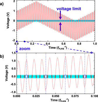
Figure 2. Picture (a) shows schematically the combined generator's high frequency sine wave and the triangular Josephson signal. (b) Sampled data within a specified voltage limit (here ±0.1 V) are selected to calculate the RMS voltage of the sine wave (shaded area). Data around transients are neglected (indicated by the vertical dashed lines and blue boxes).
Download figure:
Standard image High-resolution imageIt is not necessary to capture a whole cycle of fmeas on one PJVS step. The parameters that need to be established are: (1) fPJVS (2) the number of steps per period in the Josephson waveform (40) (3) the ADC sample rate fSa (4) fmeas must be a multiple of fPJVS (excluding number of steps × fPJVS to avoid incomplete reconstruction) and fit n (integer) times into the ADC sample rate fSa (5) the voltage limit. The phase angle between the trigger signal for the ADC and the stepwise approximated PJVS waveform needs to be known for correct reconstruction of the waveform being measured. For most frequencies a sample rate of 4 MSa s−1 has been chosen. In order to verify the results, some frequencies have been measured using a sample rate of 10 MSa s−1. For signal generators with stronger amplitude variations in frequency than the Fluke 5700A calibrator we used, these parameters can be determined starting with fmeas.
2.3. Filter function
We group the complete transfer function of the sampler, its analogue input filters and amplifiers and any digital filters under the name of filter function. Strictly speaking, our filter function evaluates the impact on the measurement of the RMS value of the magnitude and phase components of the transfer function. We have explored two samplers for the extension of the ac-QVM to higher frequencies. We investigated a 22-bit successive approximation (SAR) ADC from Applicos. A WFD22 1 [21] that can sample up to 1 MSa s−1, and continued to use an NI PXI 5922, a ΣΔ-ADC, as in our previous work [6, 7]. Further information about this sampler has been published previously [22–25]. The samplers we have studied change their transfer function significantly depending on the filter chosen. Instruments used in metrology aim for a filter function with a gain of exactly one combined with a frequency dependence of a few µV V−1. For calibrating a single tone, knowledge of the gain at this frequency is enough. In differential sampling, the signal at the input of the sampler changes from the single tone being measured to the broadband difference signal when the PJVS steps are subtracted. Figure 3 demonstrates the high number of tones present in a combined waveform, combining a 40-step triangular Josephson waveform and a 100 kHz sine wave from the calibrator. As all frequency tones must be gain-corrected simultaneously, the filter function in the sampler plays a crucial role.
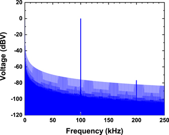
Figure 3. Frequency spectrum for the quantum voltmeter in the sub-sampling mode when a 100 kHz sine wave is measured using a triangular Josephson waveform with 40 steps at 20 Hz.
Download figure:
Standard image High-resolution imageThus, it is important to precisely describe the filter function. This is a challenging task as a perfect description of e.g. the 48-tap finite-impulse-response (FIR) filter in the NI PXI 5922A requires many parameters. In addition, filter functions depend on the instrument voltage range and sample rate settings. Thus, we performed a measurement to calibrate the filter function for each setting used. Then we either tried to find a closed-form or a numerical description of the filter function.
For measuring the filter function, the 1 V output voltage of a synthesizer (Keithley 3390 1 ) is applied to the input of the ADC. This synthesizer has a maximum frequency of 20 MHz whereas the 5700A calibrator reaches 1 MHz. A frequency sweep is performed by stepping up to the Nyquist frequency, 0.5 × fSa , in steps of either 500 Hz or 1 kHz. These sweeps are time consuming even with short waiting times of 20 s after each frequency change. A Fluke 792A 1 was connected in parallel to track the output voltage of the synthesizer. To confirm that the input resistance and capacitance of the Fluke 792A in parallel to the input of the ADC has little influence on the readings, a second sweep has always been performed. In this second sweep a (previously calibrated) calibrator was connected directly to the ADC such that the frequency range of the calibrator (1 MHz) could be covered. The two methods always agree very well up to 1 MHz within an overall uncertainty of about 50 µV V−1. As shown in section 4, this uncertainty for characterizing the filter function is adequate to reach µV V−1 uncertainties in the differential sub-sampling measurements of the RMS value.
Figures 4 and 5 show some filter function examples for an SAR-ADC and a ΣΔ-ADC, respectively. The frequency dependence for the SAR-ADC (Applicos WFD22 1 on the 6.8 Vpp range at 1 MSa s−1 and filter set to 'bypass' [21]) is easy to describe. We used a 9th-order polynomial filter function for frequencies up to 0.44 × f/fSa . The fit and the measurement agree always within 40 µV V−1as shown by the residuals (blue line) in figure 4.
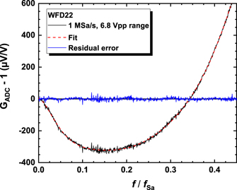
Figure 4. Frequency behavior of the WFD22 6.8 Vpp range at a sample rate of 1 MSa s−1 and 'bypass' filter setting. The frequency dependence has been fitted by a 9th-order polynomial curve. The residual error is within 40 µV V−1for the full bandwidth.
Download figure:
Standard image High-resolution image
Figure 5. Normalised frequency behavior of the 5922A 10 V range for the sample rates 4 MSa s−1, 10 MSa s−1 and 15 MSa s−1 and 48-tap filter setting.
Download figure:
Standard image High-resolution imageAs an example, the filter functions for three different sample rates 4 MSa s−1, 10 MSa s−1 and 15 MSa s−1 on the 10 V range using the '48-tap standard' FIR filter setting are shown for the ΣΔ-ADC in figure 5. These functions are more difficult to describe. Obviously, the sample rate has a large influence on the maximum deviation from the nominal value. We found that for 4 MSa s−1 this deviation is smallest. Assuming a similar quality for the filter fit function as in the SAR case this sample rate should give us the smallest corrections and therefore will lead to better results.
As pointed out above, the broadband nature of the difference signal acquired by the ADC requires that the fit matches closely the filter function. We compared more than 10 closed-form descriptions of filter functions. An example of such a fit is shown on figure 6(a). At low frequencies the filter function is matched with the fit within 50 µV V−1 as shown by the residual blue line. Due to the complicated waveform we typically observe deviations between measurement and fit in the frequency range 0.35–0.45 × f/fSa . Measurements up to 125 kHz cover only a small part up to 0.03125 × f/4 MSa s−1 (see the pink-colored areas in figure 6). On the right-hand side a numerical fit is used. As it is impossible to only use one polynomial fit the frequency range was divided into 5 parts and each part was fitted by a 7th-order polynomial. Except a small kink at 0.4 × f/fSa the filter function is well fitted. It is important to note here that filter function corrections need a smooth behavior at frequencies above 0.4 × fSa. Otherwise high frequency components in the combined waveform will be overvalued and corrupt the result.

Figure 6. Filter function of the 5922A 10 V range at 4 MSa s−1 sample rate and tap-48 filter setting (black lines). (a) The frequency dependence has been fitted using a closed-form function (red line). (b) The frequency dependence has been fitted by five 7th-order polynomials for the segments indicated by the light grey vertical lines at 0.1 × fSa (dashed orange line). The residual errors are shown by the blue curves. The pink shaded area shows the frequency band up to 125 kHz.
Download figure:
Standard image High-resolution image2.4. Cable error and correction
Cable error analysis is crucial for Josephson standards as the quantum-based accuracy can be spoiled by long cables between liquid helium temperatures and the instruments at room temperature. As already mentioned, the extension of the ac-QVM to higher frequencies requires considering and analyzing additional error components. The length of the cable connecting the PJVS, the generator and the sampler is one such error contribution. Previously cable errors have been studied by transmission line experiments and simulation [13, 25–29], with additional extrapolation [30–32] or an impedance matching method [33]. Figure 7 shows the detailed set-up that we used to analyze the cable error for the Josephson-referenced sub-sampling method. The Josephson array was set to its zero step to determine the difference in cable correction for the 2.60 m long cable between generator, Josephson array and sampler relative to a 0.40 m cable and no PJVS. A switch is introduced to measure the difference arising from two cable lengths. Be aware that the set-up has been slightly changed in comparison to a formerly reported one [14] with a different PJVS bias source and the sampler now measures the cable error. Also, the cable lengths have been slightly modified, especially to incorporate a choke indicated by the red ring in figure 7. The PJVS bias source, including its power supply, does not change the cable length but, due to its capacitance to ground (likewise indicated in figure 7), it changes reflections and thus greatly influences the cable error measurement [13, 32]. With little variation between specific Josephson bias source (NPL or Active Technologies) and its power supply, we observed an increase of the cable error by a factor of 1.5–2.5 when connected although the PJVS is on the zero step. This means that the effective cable length is increased from 2.60 m to about 5.2 m by the bias source and cables. The remaining error due to the finite reference lengths can be estimated for 100 kHz as 285 µV V−1 × (f/100 kHz)2 × (lshort/lPJVS)2 ≈ 285 µV V−1 × 0.402/5.22 ≈ 1.7 µV V−1. This systematic error has been subtracted from all measurement data. It is worth mentioning here that the choke is important to reduce the influence of the detector's input impedance. Figure 8(a) shows the repeatability of the cable error at 100 kHz over a period of three days. All measurements are stable within ±4.5 µV V−1 at a level of 285 µV V−1. However, day-to-day variations can be as large as 6.5 µV. This is something we expected because the cable error is subject to many parameters e.g. depends on the helium level inside the dewar [28]. Therefore, we kept the switch in place to trace these changes. Before and after each measurement the set-up of figure 7 was used to measure the cable error. Afterwards, the cable error was fitted (the residuals are shown in figure 8(b)) and the resulting fit was subtracted from the sub-sampling data. As expected, the cable error mainly increases quadratically with frequency up to 100 kHz [26–33], but also has a small linear term [13]. Such a fit describes the cable error well within ±2 µV V−1 for frequencies from 500 Hz to 100 kHz. Nonetheless measurements at 125 kHz are very often outliers from the corresponding sweeps. A more sophisticated analysis including all cable lengths, the switch, the array (inductance), parallel capacitances (bias source) and the input impedance of the detector is required to improve the understanding of all components in the cable error setup and thus the uncertainty. We leave this for a future investigation.
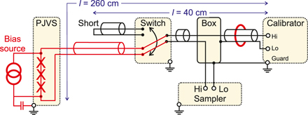
Figure 7. Schematic diagram of the set-up to investigate the influence of cable length.
Download figure:
Standard image High-resolution image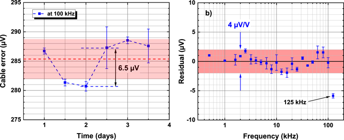
Figure 8. Cable error measurements. (a) Repeatability investigation of the cable error at 100 kHz over 3 days. (b) Residuals for the fit of cable error as a function of frequency.
Download figure:
Standard image High-resolution image2.5. Conventional calibration of the calibrator
Our main signal generator for this work, a Fluke 5700A calibrator, was calibrated conventionally by ac–ac measurements using a Fluke 792A thermal transfer standard. The output voltage of the calibrator at 100 kHz, measured with a Fluke 8588A voltmeter, does not change for loads larger than 400 Ω, so the frequency response from the calibration with the 792A is applicable to the ac-QVM sub-sampling measurements. Figure 9 shows the frequency-dependent relative deviation of the Fluke 792A from the nominal value for frequencies up to 300 kHz measured with a constant 1 V nominal amplitude at the generator. The dashed purple line is a fit to this calibration. Two measurements of the Fluke 5700A calibrator using the Fluke 792A and performed in April 2018 and April 2020, are shown. Both measurements agree very well within a few µV V−1. It is important to mention that the calibrator was synchronized using a sine wave with amplitude of 3 V RMS. This amplitude has also been used for all measurements, because we observed a small, 2.3 µV V−1, voltage output change when varying the synchronization amplitude by 1 V at 100 kHz. Slightly above 100 kHz a jump of the calibrator output voltage is visible due to an internal range switching. In order to extract the frequency dependence of the 5700A calibrator from these measurements, figure 9 also shows selected data points, in purple, from a recent calibration with multi-junction thermal converters up to 1 MHz. The dashed line shows a fit to these data points. A typical variation of these thermal converter results in the 2.2 V range for a 1 V amplitude at 100 kHz is within ±2.5 µV V−1 for all the calibrations that have been performed since 1990.

Figure 9. Relative voltage change of the Fluke 5700A calibrator as function of frequency for 1 V measured with a Fluke 792A thermal transfer standard. Selected points from the conventional calibration of the 792A and a fit for its frequency dependence are shown in purple.
Download figure:
Standard image High-resolution imageA traceable frequency response for the Fluke 5700A was obtained by correcting the measurements by the calibrated values of the Fluke 792A thermal transfer standard. The next figure (figure 10(a)) shows this calibration for the Fluke 5700A 1 . The blue-dashed-line fit describes the deviation of the calibrator from a perfectly flat frequency dependence up to 100 kHz. This fit has been used to correct all following measurements i.e. a perfect measurement with the ac-QVM should not deviate from the nominal value 0 µV V−1 as shown by the residuals of the fit (red) in figure 10(b), which also includes a moving average in black.

Figure 10. (a) Relative voltage deviations to the thermal transfer standard for the calibrator at 1 V. The voltage deviation measurement (red) has been fitted (blue dashed line). (b) Our reference values for other measurements have been achieved by subtracting the fitted line from the conventional calibration (red line). For clarity a moving average is added (black line).
Download figure:
Standard image High-resolution image3. Measurement results
3.1. Sub-sampling measurement results
The measurement procedure and calculation of RMS values followed the routines described for the differential measurement principle [6]. Before starting measurements, the dc offset and the ADC's gain at fPJVS are determined within a few minutes using the Josephson waveform synthesizer to generate a stepwise approximated waveform with 1.4 V peak amplitude. Any offset voltage due to thermals is easily detectable and the gain is measured by a linear fit to the voltage steps [6, 7]. The combined signal of Josephson stepwise triangular waveform and calibrator sine wave is then sampled for several fPJVS periods by the ADC and averaged. These data are instantly transformed into the frequency domain and corrected according to the filter function. Afterwards the inverse fast Fourier transform is used to transfer the signal back into the time domain. Then the waveform is reconstructed by adding the corresponding Josephson voltages, as in [6]. For sub-sampling only the phase of fPJVS relative to the sampling frequency fSa must be adjusted carefully. The relative phase angle between the high frequency signal fmeas and fPJVS is not important, but the minimum voltage limit for accepting data (as shown schematically in figure 2 with rounded numbers) must be set carefully. This limit depends on the number of Josephson steps. At high frequencies the voltage limit for 40 Josephson steps is 0.071 V. Towards lower measurement frequencies fewer sampling data are close to Josephson steps, so the voltage limit must be increased to reconstruct the sine wave. The limit for 500 Hz with 40 steps at fPJVS = 20 Hz must be set to 0.15 V, or 2.1 times larger than at 100 kHz. Such an increase requires a proper setting of the ADC gain to avoid erroneous measurements, as will be explained in section 4.
For the WFD22, measurements with 180 readings of 2 periods of fPJVS = 20 Hz or 250 readings of 2 periods at fPJVS = 62.5 Hz take about 300 seconds. Such a timing is optimized in all our measurements by applying an Allan deviation analysis [34]. Thus, a complete, automated frequency sweep with about 20 frequencies requires approximately 100 minutes. Overnight measurements typically include 10 such loops. Figure 11 shows measurements with the WFD22 using a Josephson triangle waveform of 20 Hz or 62.5 Hz and sample rates of 0.96 MSa s−1 and 1 MSa s−1. As fSa must be a multiple of fmeas and fmeas a multiple of fPJVS, we used different combinations to acquire more data points in the high frequency range e.g. at 80 kHz. Due to the low sample rate around 1 MSa s−1 only 10 data points contribute to the calculation of the RMS values at 100 kHz and the quite low data transfer rate results in increasing type-A uncertainties (k = 1), the error bars in figure 11, as the frequency rises. The measurements include the corrections detailed in sections 2.3 to 2.5 for the filter function, cable error and frequency dependence of the calibrator. All measurements spread around the nominal value and are within the grey areas which indicate best calibrator specifications (k = 1).

Figure 11. Results of sub-sampling up to 100 kHz at 1 V showing the voltage difference of the measured voltage Vmeas and the nominal value of the Fluke 5700A calibrator Vnom. Grey areas indicate the type-A uncertainties (k = 1) of the 5700A from its specifications.
Download figure:
Standard image High-resolution imageFor the measurements with the NI 5922 the spread of the data is much smaller (figures 12 and 13). Up to 100 kHz all measurement points are within ±5 µV V−1 of the nominal value. The type-A error bars increase from below 1 µV V−1 at 1 kHz to 2 µV V−1–3 µV V−1 100 kHz. A measurement with 100 readings of 10 periods at fPJVS = 20 Hz takes typically 70 seconds as do 300 readings of 10 periods at fPJVS = 62.5 Hz. A complete frequency sweep with 20 frequencies requires approximately 30 minutes. Such sweeps are typically repeated 10 times for one set of parameters.
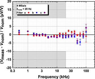
Figure 12. Results of sub-sampling up to 100 kHz at 1 V for the voltage difference Vmeas and the nominal value of the Fluke 5700A calibrator Vnom with the NI 5922 sampling at 4 MSa s−1. Three different filter functions ((a) and (b) of figure 6) are used for a frequency fPJVS = 20 Hz and a sample rate of 4 MSa s−1. The error bars indicate type-A uncertainties (k = 1). The grey area marks the specification of the 5700A.
Download figure:
Standard image High-resolution image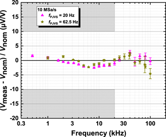
Figure 13. Results of sub-sampling up to 100 kHz at 1 V using two frequencies, fPJVS, 20 Hz and 62.5 Hz, at a sample rate of 10 MSa s−1. The measured voltage Vmeas is plotted as difference to the nominal value of the Fluke 5700A calibrator Vnom. A new polynomial filter function is used (see figures 5 and 6(b)). The error bars indicate type-A uncertainties (k = 1).
Download figure:
Standard image High-resolution imageFigure 12 shows a summary of such sweeps where three different filter correcting functions have been used at 4 MSa s−1 with fPJVS = 20 Hz. Within the variation of ±3 µV V−1 no significant difference between the filter correcting functions a, b and c is visible. Very similar curves are achieved with a sample rate of 10 MSa s−1, two Josephson frequencies, fPJVS = 20 Hz and fPJVS = 62.5 Hz, and another filter function (figure 13). A possible reason for the relatively high deviations at 500 Hz (up to 2.4 µV V−1 see figures 12 and 13) could be due to a small remaining frequency dependence of the calibrator, see figure 10(b) and e.g. [6]. The measuring time of the differential sub-sampling ac-QVM with the NI 5922 is dominated by the number of periods of fPJVS acquired. As a result, direct differential ac-QVM produces comparable or lower uncertainties in shorter measuring times without the limitation for the input range of the sampler for frequencies up to several kHz. Finally, figures 12 and 13 seem to indicate a remaining frequency behavior but we cannot conclude here if this behavior is significant for our uncertainty estimations. An uncertainty budget for the ac-QVM measurements at 100 kHz is presented in the next section.
4. Uncertainty investigations
As demonstrated in the last section, the measurement results using the NI PXI 5922 ADC are within ±5 µV V−1 to the value predetermined by the conventional traceability up to 100 kHz. Here we present a number of investigations in order to validate the performance of the sub-sampling ac-QVM thoroughly. The uncertainty budget for the ac-QVM sub-sampling technique was also evaluated and is given in table 1 for 100 kHz. All uncertainty components are discussed in this section.
Table 1. Uncertainty budget for the ac-QVM at 100 kHz (k = 1)
| Component | Estimate (µV V−1) | Distribution | Uncertainty (µV V−1) |
|---|---|---|---|
| Type-A | |||
| Noise (10 minutes) | 1.5 | Normal | 1.5 |
| Type-B | |||
| Josephson system | 0.001 | Normal | 0.001 |
| Voltage limit | 1.0 | Rectangular | 0.58 |
| Sampler gain | 0.17 | Rectangular | 0.1 |
| Sampler filter function | 3.2 | Rectangular | 1.8 |
| Cable correction | 3.25 | Rectangular | 1.9 |
| Calibrator calibrated value | 3.0 | Rectangular | 1.7 |
| Total | 3.5 |
The combined uncertainty for the sub-sampling ac-QVM at 1 V RMS and 100 kHz is 3.5 µV V−1 (k = 1). This frequency represents the worst-case scenario for the method. Lower frequencies profit from slightly lower uncertainty contributions e.g. cable correction and sampler filter function are negligible at 500 Hz. An uncertainty estimation for the sub-sampling ac-QVM at 1 V RMS and 500 Hz is 1.0 µV V−1 (k = 1).
The type-B contributions solely from the ac-QVM at 100 kHz (e.g. without uncertainties for type-A and the calibrator calibrated/nominal value) result in an uncertainty of 2.7 µV V−1 (k = 1). The contribution due to the Josephson system is almost negligible [6]. The other type-B contributions to the uncertainty budget are discussed in detail in the following paragraphs.
4.1. Sampler gain
In order to estimate the error due to the gain setting, GADC, of the sampler, specific measurement loops were performed. We reconstructed the waveform at the input of the ac-QVM and deliberately changed the gain by ± 2 × 10⁻³ when sub-sampling a 1 kHz sine wave using 40 triangular Josephson steps at 20 Hz. A similar gain error measurement has been performed and reported in detail in [11]. As expected, the voltage deviations follow the gain variation linearly. Due to the differential sub-sampling method, the influence of the gain error is suppressed by a factor of about 285, from 2 × 10⁻³ V V−1 to 7 µV V−1, compared to the case when the sampler and its internal voltage reference are used to measure the waveform directly [35]. An absolute maximum error for the reconstructed RMS value can be estimated by a conservative ± 50 µV V−1 gain variation during measurements. Assuming a rectangular distribution we achieve an uncertainty uG = 50 µV V−1/285/√3 = 0.1 µV V−1 (k = 1).
4.2. Voltage limit
Defining the number of Josephson steps involved in the low frequency triangular stepwise waveform requires setting a voltage limit for the reconstruction of the high frequency sine wave. As explained in section 2.2, the voltage limit depends on the frequency being measured and changes from 0.15 V at 500 Hz to 0.08 V above 3 kHz (40 steps at fPJVS = 20 Hz). Figure 14 shows the relative error in the RMS value of the calibrator at 500 Hz and 10 kHz for different voltage limits and a deliberately changed gain by ±5 × 10⁻⁵. This plot demonstrates an obvious behavior—errors increase with increasing voltage limit if the gain is set incorrectly. Once the limit is set to the minimum value required to acquire the complete period of fmeas, errors decrease to the noise limit of the measurement. As a result, we chose the smallest voltage limit possible and the gain was calibrated (with the PJVS steps, as explained in section 3.1) and changes by less than ±50 µV V−1 during each set of measurements. All experimental values at low voltage limits in figure 14 are within 1 µV V−1. Therefore, for 100 kHz using 0.08 V as voltage limit, we estimate an uncertainty uL = 1 µV V−1/√3 = 0.58 µV V−1 (k = 1).
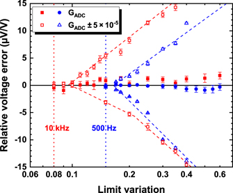
Figure 14. Relative errors in the measurement of the calibrator for a deliberately changed gain of the sampler and the voltage limit for collecting data in the sub-sampling mode.
Download figure:
Standard image High-resolution image4.3. Sampler filter function
By conducting measurements with three different filter functions at 4 MSa s−1 and another one at 10 MSa s−1, possible errors due to erroneous corrections of filter functions should have been visible. These measurements up to 100 kHz agree very well within ±3 µV V−1 (figure 12) even though the filter functions differ in the high frequency range. Furthermore, deviations could be partly obscured due to other errors like e.g. cable correction, type A, or the calibrator nominal value and a clear separation of these contributions is difficult. One solution would be to use a set of raw data and to make a robustness test with Monte Carlo simulation. Due to the large number of parameters in the filter functions and the large data sets such an investigation would be very time consuming and beyond the scope of this paper.
To estimate the impact of the sampler filter correction impact on the measurement results we deliberately varied the gain of the filter function by ±10−4, as shown by the shaded area in figure 15(a), which results in the variations in RMS values shown on figure 15(b). In the frequency range 2 kHz to 100 kHz, the voltage deviation is within ±1.1 µV V−1. Type-A uncertainties (k = 1) are of the order of 0.5 µV V−1 at low frequencies and 1.5 µV V−1 at 100 kHz (not shown for clarity). From this investigation we can conclude that the calibration of the filter function with an uncertainty below 100 µV V−1 affects the reconstructed RMS value by less than 1.1 µV V−1. We have seen that very different filter functions (especially in the high frequency filter range) influence the measurements by up to ±3 µV V−1, so we can conclude that a good description of the complete bandwidth is very important. An uncertainty estimation of √(1.12 + 32)/√3 µV V−1 = 1.8 µV V−1 can be given for the filter function.

Figure 15. (a) The shaded area illustrates the effect of deliberately varying the filter function by ±10−4. (b) Impact of the gain variation on the reconstructed RMS value.
Download figure:
Standard image High-resolution image
4.4. Cable correction uncertainty
Typically, the cable error for liquid-helium based Josephson voltage standards at 100 kHz is of the order of 200 µV V−1 [30]. Due to the increase in cable length from the choke and stray capacitances from the Josephson bias source to ground, the cable error is increased to 285 µV V−1 at 100 kHz. Therefore, it is crucial to keep the setup unchanged between calibrations and cable error measurements using the proposed correction method. As mentioned before the cable error depends on helium level such that over a measurement campaign with one 100 l helium dewar we observed day-to-day changes of up to 6.5 µV V−1. Having a switch included in the measurement line allows us to track these changes. In section 2.4, we established a systematic error due to the minimum cable length of 1.7 µV V−1 at 100 kHz. This systematic error has been subtracted from all data, however, the uncertainty for this correction must be considered. Assuming a cable length error of 0.02 m (5%) it results in a systematic error of 0.15 µV V−1 at 100 kHz. Another systematic error due to the switch has been found in [13]. The error is less than 2 µV V−1 at 500 kHz resulting in an uncertainty of 2 µV V−1/(500 kHz/100 kHz)2 = 0.08 µV V−1 at 100 kHz. Performing these cable correction measurements before and after each measurement set, we calculate from the maximum day-to-day variation of ±3.25 µV V−1 in figure 8 an uncertainty of 3.25 µV V−1/√3 = 1.9 µV V−1.
4.5. Calibrator nominal value
For the demonstration of the new sub-sampling method the calibrator is used as the device under test and the uncertainty contribution of the conventional calibration is not relevant for the ac-QVM. However, as we want to validate the new sub-sampling method by comparing it with the conventional calibration of the calibrator using a Fluke 792A we need to estimate the uncertainty for that calibration. The nominal value of the calibrator has been traced regularly by comparing it to a Fluke 792A. The Fluke 792A itself has been calibrated routinely from time to time. The plots in section 2.3 demonstrate that the repeatability of the calibration results is within ±3 µV V−1 over years. This is much better than the manufacturer's specification [36]. However, based on our calibrations we only can estimate an upper uncertainty limit of 3 µV V−1/√3 = 1.7 µV V−1.
5. Conclusion
We have implemented a new sub-sampling technique to extend the frequency range of our ac-QVM up to 100 kHz for the first time. The new technique was easily incorporated into existing, highly automated measurement procedures. This will help to exploit the new method by other national metrology institutes or calibration laboratories.
The ac-QVM measurement results agree well within ±5 µV V−1 with the calibrator's calibrated voltage values for all frequencies for amplitudes of 1 V. A combined uncertainty of 3.5 µV V−1 (k = 1) has been determined for the comparison at 100 kHz. The measurement setup, the techniques employed, error sources and corrections as well as uncertainty estimations were discussed. Although the extension has been demonstrated at the 1 V level, larger amplitudes can also be measured. The limitation, however, is the maximum input range of the ADC that must accommodate the sum of the amplitude being measured and the peak value used from the PJVS.
The integration of a switch allowed us to determine cable errors with an uncertainty of a few µV V−1 for each set of measurements. Such an uncertainty is comparable to other cable error correction methods [27–33, 37]. Combining the switch method with one of the other methods could be a way to further improve the determination of cable errors and their correction.
The measurement uncertainty without the contribution from the device under test was 2.7 µV V−1 (k = 1) at 100 kHz. This uncertainty is comparable to those of ac-dc transfer standards, which are in the range of 2 µV V−1–3 µV V−1 [38]. However, calibrations could be much faster (less than ten minutes compared to one hour) and can provide additional waveform parameters instead of just the RMS value.
In the future the uncertainty of the ac-QVM could be advanced especially when using a pulse-driven Josephson voltage standard as quantum-based synthesizer to further validate the sub-sampling method. Vice versa the high-quality ac-QVM could also help to further improve pulse-driven Josephson voltage standards e.g. for investigating crosstalk at kHz frequencies [11].
Acknowledgments
The authors would like to acknowledge Franz Ahlers, Jinni Lee and Susanne Gruber for programming support, Alexander Katkov (VNIIM), Marco Schubert (Supracon), Mun-Seog Kim (KRISS), Stéphane Solve (BIPM), Jan Kucera (CMI), Stephan Bauer, Marco Kraus, Torsten Funck, and Susanne Weimann (all PTB) for valuable discussions and for the conventional calibrations. Furthermore, we thank Rüdiger Wendisch, Gerd Muchow, Torsten Stöcker and Michael Busse (all PTB) for technical support.
Footnotes
- 1
Identification of commercial equipment does not imply an endorsement by PTB or that it is the best available for the purpose.