Comparison of DSSP and tSSS algorithms for removing artifacts from vagus nerve stimulators in magnetoencephalography data

Chang Cai; Huicong Kang; Heidi E Kirsch; Danielle Mizuiri; Jessie Chen; Abhishek Bhutada; Kensuke Sekihara; Srikantan S Nagarajan

doi:10.1088/1741-2552/ab4065

1. Introduction

Magnetoencephalography (MEG) has made a tremendous impact on noninvasive brain mapping because it provides good spatial and excellent temporal resolution and can offer valuable information for use in clinical neurology and in basic neuroscience. Unfortunately, the strength of brain MEG activity is typically 50–1000 fT, and MEG recordings are prone to contamination arising from inevitable non-biological sources such as power lines and trains, and from biological sources outside the brain, for example the heart. Although most of this interference is of a similar magnitude to brain activity, some can be quite large, arising from magnetic fields in the environment or even from the patient's own body or head, including, for example, artifacts from dental work. A prototypical example is the interference arising from vagal nerve stimulator (VNS) implants in patients with intractable epilepsy—VNS artifacts make it very difficult for us to consistently and reliably detect and localize epileptiform activity in such patients [1–3].

The preferred way to deal with interference from the environment is to prevent it. If this is not possible a variety of methods have been applied to minimize artifacts in MEG recordings. One commonly used method is to apply high-pass or band-pass filters. However, the brain signal of interest may be in the same frequency range as the artifact, so filtering may not be effective. One can also reject trials that contain large artifacts; however, this may cause unacceptable loss of signal from the brain [4]. Another commonly used method is averaging responses over trials: the fundamental idea behind this is that interference in different trials is statistically independent, whereas evoked signals are not. However, this method requires a large number of trials, and evoked signals must be relatively similar and robust [5].

Recently, data-driven approaches such as principal component analysis (PCA) and independent component analysis (ICA) have been used for the removal of artifacts. However, these methods require users to make subjective choices during application (e.g. choice of threshold in PCA; selection of interference components for removal in ICA) [6, 7]. Joint decorrelation is another method commonly supposed to be robust to many types of interference problems, but its use requires the design of different bias filters for different interference types, and thus to some extent requires prior knowledge of the interference [8].

Ideally, any interference removal algorithm would be robust and broadly capable of rejection of as many types of interference as possible. Currently, options are restricted to specific MEG hardware platforms. For example, in the Elekta platform, the temporally extended signal space separation (tSSS) method was developed based on spherical harmonic decomposition, and offers a potential solution [4]. However, the validity of this method has only been demonstrated for Elekta and has not been shown for other hardware platforms. Recently, we proposed a MEG hardware platform-independent algorithm named dual signal subspace projection (DSSP) for removal of large interference in biomagnetic measurements. In a retrospective clinical study we have shown the potential of DSSP to deal with high-amplitude periodic interference. DSSP helps to recover distorted MEG recordings from people with intractable epilepsy and VNS implants, making identification of epileptic spikes easier and improving spike mapping [3, 9].

The performance of DSSP and tSSS has not been directly compared. In this study we compare the performance of these two algorithms using simulated data and real MEG recordings from patients with VNS implants. We test the algorithms' ability to remove interference from resting-state MEG data in patients with VNS implants and also to improve source localization of somatosensory evoked fields (SEFs) using Champagne, an empirical Bayesian source reconstruction algorithm described previously [10]. Results show that DSSP and tSSS algorithms have a similar performance for interference rejection. However, for the tSSS algorithm to have comparable performance to DSSP the origin location for the spherical harmonic decompositions must be set properly. Section 2 briefly describes the DSSP and tSSS algorithms. Section 3 describes the computer simulation used for performance comparison, followed by a description of their performance on real data analysis in section 4. Section 5 provides a short discussion followed by a conclusion in section 6.

2. Methods

2.1. Structure of the DSSP and tSSS algorithms

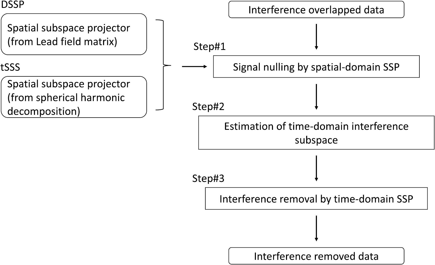
This section briefly describes the DSSP and tSSS algorithms. Detailed explanations of these algorithms have been published [2, 3, 11]. These algorithms share a common structure outlined in figure 1. As shown in this figure, these algorithms consist of three steps: signal nulling, estimation of time-domain interference subspace and time-domain signal space projection (SSP) [11]. The signal nulling step involves projecting out the signal components from the measured sensor data by applying the spatial-domain SSP algorithm [12, 13], i.e. by projecting the data matrix onto the subspace orthogonal to the signal subspace, which is called the noise subspace. This procedure is referred to as signal nulling in this paper, and the operator used for it is called the signal nulling operator.

**Figure 1.** Conceptual sketch of the DSSP and tSSS algorithms.
Download figure:
Standard image High-resolution image

Theoretically, the noise subspace projector is an ideal signal nulling operator. However, since the signal and noise subspace projectors are unknown, we must use something that can substitute for these projectors. For this, the DSSP algorithm uses the pseudo-signal subspace projector $\newcommand{\brcPS}{\breve{\boldsymbol{P}}_S} \brcPS$ defined in equation (A.4) in the appendix. The tSSS algorithm uses the SSS internal subspace projector $\newcommand{\vP}{\boldsymbol{P}} \newcommand{\vPi}{\boldsymbol{\Pi}} \newcommand{\vPint}{\boldsymbol{P}_{\mathrm{int}}} \vPint$ defined in equation (B.19), the derivation of which is described in detail in appendix B.

When using $\newcommand{\vP}{\boldsymbol{P}} \newcommand{\vPi}{\boldsymbol{\Pi}} \newcommand{\vPint}{\boldsymbol{P}_{\mathrm{int}}} \vPint$ , the internal region needs to be matched with the source space⁷, and this matching between the internal region and the source space can be attained by setting the origin for the spherical harmonics decomposition at a proper location. Note that the location of this origin is a parameter that should be specified by the user when implementing the tSSS algorithm. This is because the tSSS algorithm computes the SSS basis vectors using the spherical polar coordinate with this origin, and then derives $\newcommand{\vP}{\boldsymbol{P}} \newcommand{\vPi}{\boldsymbol{\Pi}} \newcommand{\vPint}{\boldsymbol{P}_{\mathrm{int}}} \vPint$ using the SSS basis vectors. Thus, this origin of the polar coordinate is called the SSS origin in this paper. If the location of the SSS origin is not properly set, a mismatch between the source space and the internal region arises that can cause a significant distortion in the interference removal results of the tSSS algorithm, as shown in our computer simulation in section 3.

Note that the only practical difference between the DSSP and tSSS algorithms is in the manner of approximating the signal subspace projector in the first step; the subsequent steps are exactly the same for these algorithms. The second step estimates the interference subspace by computing the intersection between the row spaces of the two modified data matrices obtained with and without signal nulling. The third step implements the time-domain SSP by using the interference subspace projector estimated in the second step. These two steps are further explained below.

2.2. Estimation of interference subspace and interference removal

Regarding interference removal, the model for the measured data is defined in a matrix form such that

$\begin{align} \newcommand{\e}{{\rm e}} \newcommand{\vBep}{\boldsymbol{B}_{\vep}} \newcommand{\vBI}{\boldsymbol{B}_I} \newcommand{\vBS}{\boldsymbol{B}_S} \newcommand{\ve}{\boldsymbol{e}} \newcommand{\vB}{\boldsymbol{B}} \newcommand{\vep}{\boldsymbol{\varepsilon}} \newcommand{\va}{\boldsymbol{a}} \displaystyle \label{mdmodel} \vB = \vBS + \vBI + \vBep , \nonumber \end{align} \tag{ 1 }$

where $\newcommand{\vB}{\boldsymbol{B}} \vB$ is the data matrix, $\newcommand{\vB}{\boldsymbol{B}} \newcommand{\vBS}{\boldsymbol{B}_S} \vBS$ is the signal matrix, $\newcommand{\vB}{\boldsymbol{B}} \newcommand{\vBI}{\boldsymbol{B}_I} \vBI$ is the interference matrix and $\newcommand{\va}{\boldsymbol{a}} \newcommand{\vep}{\boldsymbol{\varepsilon}} \newcommand{\vB}{\boldsymbol{B}} \newcommand{\ve}{\boldsymbol{e}} \newcommand{\vBep}{\boldsymbol{B}_{\vep}} \vBep$ is a sensor noise matrix. The approximate signal subspace projector is denoted by $\newcommand{\hvPS}{\widehat{\boldsymbol{P}}_S} \hvPS$ , which is equal to $\newcommand{\brcPS}{\breve{\boldsymbol{P}}_S} \brcPS$ in the DSSP algorithm and $\newcommand{\vP}{\boldsymbol{P}} \newcommand{\vPi}{\boldsymbol{\Pi}} \newcommand{\vPint}{\boldsymbol{P}_{\mathrm{int}}} \vPint$ in the tSSS algorithm. This $\newcommand{\hvPS}{\widehat{\boldsymbol{P}}_S} \hvPS$ satisfies the relationship $\newcommand{\vB}{\boldsymbol{B}} \newcommand{\hvPS}{\widehat{\boldsymbol{P}}_S} \newcommand{\vBS}{\boldsymbol{B}_S} \hvPS \vBS \approx \vBS$ and the signal nulling operator is obtained as $\newcommand{\vI}{\boldsymbol{I}} \newcommand{\hvPS}{\widehat{\boldsymbol{P}}_S} \vI - \hvPS$ . The both DSSP and tSSS algorithms modify the measured data matrix in two ways by applying $\newcommand{\hvPS}{\widehat{\boldsymbol{P}}_S} \hvPS$ and $\newcommand{\vI}{\boldsymbol{I}} \newcommand{\hvPS}{\widehat{\boldsymbol{P}}_S} \vI-\hvPS$ to $\newcommand{\vB}{\boldsymbol{B}} \vB$ , resulting in

$\begin{align} \newcommand{\e}{{\rm e}} \newcommand{\vBep}{\boldsymbol{B}_{\vep}} \newcommand{\vBI}{\boldsymbol{B}_I} \newcommand{\vBS}{\boldsymbol{B}_S} \newcommand{\hvPS}{\widehat{\boldsymbol{P}}_S} \newcommand{\ve}{\boldsymbol{e}} \newcommand{\vBin}{\boldsymbol{B}_{\mathrm{in}}} \newcommand{\vB}{\boldsymbol{B}} \newcommand{\vep}{\boldsymbol{\varepsilon}} \newcommand{\va}{\boldsymbol{a}} \displaystyle \label{bin0} \vBin=\hvPS \vB = \vBS + \hvPS \vBI +\hvPS \vBep, \nonumber \end{align} \tag{ 2 }$

$\begin{align} \newcommand{\e}{{\rm e}} \newcommand{\vBep}{\boldsymbol{B}_{\vep}} \newcommand{\vBI}{\boldsymbol{B}_I} \newcommand{\hvPS}{\widehat{\boldsymbol{P}}_S} \newcommand{\ve}{\boldsymbol{e}} \newcommand{\vBout}{\boldsymbol{B}_{\mathrm{out}}} \newcommand{\vB}{\boldsymbol{B}} \newcommand{\vI}{\boldsymbol{I}} \newcommand{\vep}{\boldsymbol{\varepsilon}} \newcommand{\va}{\boldsymbol{a}} \displaystyle \vBout=( \vI - \hvPS) \vB =( \vI - \hvPS) \vBI + ( \vI - \hvPS) \vBep, \label{bout0} \nonumber \end{align} \tag{ 3 }$

where $\newcommand{\vB}{\boldsymbol{B}} \newcommand{\vBin}{\boldsymbol{B}_{\mathrm{in}}} \vBin$ and $\newcommand{\vB}{\boldsymbol{B}} \newcommand{\vBout}{\boldsymbol{B}_{\mathrm{out}}} \vBout$ are two kinds of modified data matrices obtained from $\newcommand{\vB}{\boldsymbol{B}} \vB$ .

In equations (2) and (3), we can observe that $\newcommand{\vB}{\boldsymbol{B}} \newcommand{\vBI}{\boldsymbol{B}_I} \vBI$ -related terms exist as common components in $\newcommand{\vB}{\boldsymbol{B}} \newcommand{\vBin}{\boldsymbol{B}_{\mathrm{in}}} \vBin$ and $\newcommand{\vB}{\boldsymbol{B}} \newcommand{\vBout}{\boldsymbol{B}_{\mathrm{out}}} \vBout$ . The row spaces of $\newcommand{\vB}{\boldsymbol{B}} \newcommand{\hvPS}{\widehat{\boldsymbol{P}}_S} \newcommand{\vBI}{\boldsymbol{B}_I} \hvPS \vBI$ and $\newcommand{\vI}{\boldsymbol{I}} \newcommand{\vB}{\boldsymbol{B}} \newcommand{\hvPS}{\widehat{\boldsymbol{P}}_S} \newcommand{\vBI}{\boldsymbol{B}_I} ( \vI - \hvPS) \vBI$ are both equal to the row space of $\newcommand{\vB}{\boldsymbol{B}} \newcommand{\vBI}{\boldsymbol{B}_I} \vBI$ , which is equal to the time-domain interference subspace $\newcommand{\cK}{\mathcal{K}} \newcommand{\cKI}{\mathcal{K}_I} \cKI$ . Also, the row space of $\newcommand{\vB}{\boldsymbol{B}} \newcommand{\vBI}{\boldsymbol{B}_I} \vBI$ can be extracted as the intersection between the row spaces of $\newcommand{\vB}{\boldsymbol{B}} \newcommand{\vBin}{\boldsymbol{B}_{\mathrm{in}}} \vBin$ and $\newcommand{\vB}{\boldsymbol{B}} \newcommand{\vBout}{\boldsymbol{B}_{\mathrm{out}}} \vBout$ . Therefore, the time-domain interference subspace is obtained as

$\begin{align} \newcommand{\e}{{\rm e}} \newcommand{\vBI}{\boldsymbol{B}_I} \newcommand{\vBout}{\boldsymbol{B}_{\mathrm{out}}} \newcommand{\vBin}{\boldsymbol{B}_{\mathrm{in}}} \newcommand{\vB}{\boldsymbol{B}} \newcommand{\cKI}{\mathcal{K}_I} \newcommand{\cK}{\mathcal{K}} \displaystyle \label{bout31} \cKI = {{\rm row~space~of~}} \vBI \approx {{\rm row~space~of~}} \vBin \cap {{\rm row~space~of~}} \vBout. \nonumber \end{align} \tag{ 4 }$

The basis vectors of the intersection can be derived using the algorithm described in [11, 14]. Once the orthonormal basis vectors of the intersection, $\newcommand{\vpsi}{\boldsymbol{\psi}} \vpsi_1,\ldots,\vpsi_r$ , are obtained, we can compute the projector onto the intersection $\newcommand{\vP}{\boldsymbol{P}} \newcommand{\vPi}{\boldsymbol{\Pi}} \newcommand{\vPiint}{\boldsymbol{\Pi}\!_{X}} \vPiint$ such that

$\begin{align} \newcommand{\e}{{\rm e}} \newcommand{\vPiint}{\boldsymbol{\Pi}\!_{X}} \newcommand{\vpsi}{\boldsymbol{\psi}} \newcommand{\vPi}{\boldsymbol{\Pi}} \newcommand{\vP}{\boldsymbol{P}} \displaystyle \label{proj_dssp} \vPiint=[\vpsi_1,\ldots,\vpsi_r] [\vpsi_1,\ldots,\vpsi_r] ^T. \nonumber \end{align} \tag{ 5 }$

Using $\newcommand{\vP}{\boldsymbol{P}} \newcommand{\vPi}{\boldsymbol{\Pi}} \newcommand{\vPiint}{\boldsymbol{\Pi}\!_{X}} \vPiint$ as the projector onto the interference subspace $\newcommand{\cK}{\mathcal{K}} \newcommand{\cKI}{\mathcal{K}_I} \cKI$ , the interference removal (and as a resultant the estimation of the signal matrix) is achieved by applying the time-domain SSP:

$\begin{align} \newcommand{\e}{{\rm e}} \newcommand{\vPiint}{\boldsymbol{\Pi}\!_{X}} \newcommand{\vpsi}{\boldsymbol{\psi}} \newcommand{\hvBS}{\widehat{\boldsymbol{B}}_S} \newcommand{\vPi}{\boldsymbol{\Pi}} \newcommand{\vP}{\boldsymbol{P}} \newcommand{\vB}{\boldsymbol{B}} \newcommand{\vI}{\boldsymbol{I}} \displaystyle \label{sss_rem} \hvBS=\vB (\vI- \vPiint) = \vB(\vI-[\vpsi_1,\ldots,\vpsi_r] [\vpsi_1,\ldots,\vpsi_r] ^T), \nonumber \end{align} \tag{ 6 }$

where $\newcommand{\hvBS}{\widehat{\boldsymbol{B}}_S} \hvBS$ is the estimated signal matrix.

3. Computer simulations

As mentioned in section 2.1, the DSSP and tSSS algorithms differ in their signal-nulling operators. The tSSS algorithm uses the projector onto the SSS internal subspace as the signal-nulling operator. This SSS internal subspace projector, however, requires that the location of the SSS origin, which is a user-specified parameter, must be properly chosen. If it is not, a mismatch between the internal region and the source space could arise and this mismatch may cause signal distortion in the tSSS interference-removed results. Computer simulation in this section explores this point, and presents two kinds of examples: one in which the location of the SSS origin is properly chosen and the other in which it is not properly chosen. We then compare the results of the DSSP algorithm with those of the tSSS algorithm obtained with proper location of the SSS origin.

In our computer simulation, a sensor alignment of the 275-channel whole-head sensor array from the Omega^TM (CTF MEG Technology, Coquitlam, BC, Canada) neuromagnetometer was used. The coordinate system and source–sensor configuration used in the computer simulation are depicted in figure 2(a). We assumed a single source at a location shown by a (a black square in (a) and an orange square in (b)) in this figure; its location was presumably in the right parietal area near the primary somatosensory cortex, representing a source located near the border of the source space.

$ \newcommand{\brcPS}{\breve{\boldsymbol{P}}_S} \brcPS$ — **Figure 2.** Simulation configuration and spatial distribution of the signal gain. (a) Source–sensor configuration for the computer simulation with the two locations of the SSS origin (red circles) and the source location (black squares; orange squares in part b) (b) Plots of the spatial distribution of the signal gain. Top row: results from the projector $\newcommand{\brcPS}{\breve{\boldsymbol{P}}_S} \brcPS$ used in the DSSP algorithm (equation (A.4)). Middle row: results from the projector $\newcommand{\vP}{\boldsymbol{P}} \newcommand{\vPi}{\boldsymbol{\Pi}} \newcommand{\vPint}{\boldsymbol{P}_{\mathrm{int}}} \vPint$ used in the tSSS algorithm (equation (B.19)) with the SSS origin set at location A. Bottom row: results from the projector $\newcommand{\vP}{\boldsymbol{P}} \newcommand{\vPi}{\boldsymbol{\Pi}} \newcommand{\vPint}{\boldsymbol{P}_{\mathrm{int}}} \vPint$ with the SSS origin set at location B. Left-hand, middle and right-hand columns, respectively, show maximum-intensity projections of $\newcommand{\vr}{\boldsymbol{r}} G_S(\vr)$ onto the y –z, x–z and x–y planes.
Download figure:
Standard image High-resolution image

We assumed two locations of the SSS origin. These locations are marked as 'A' and 'B' in figure 2(a), and referred to as location A and location B in this section. Location A is 10 cm below the vertex of the sensor array, and approximately 4 cm above a typical location of the origin of a single sphere fitted to the inner border of a head MRI. The origin of this sphere is called the local sphere origin, and abbreviated as LSO in this paper. Location B is 16 cm below the vertex of the sensor array, and 2 cm below LSO. These two locations are shown by red filled circles in figure 2(a).

In order to see if these locations of the SSS origin are proper choices or not, we need to visualize where the signal nulling region exists and how widely it is extended, depending on the location of the SSS origin. For this visualization, the signal gain by the signal nulling operator was plotted. The signal gain $\newcommand{\vr}{\boldsymbol{r}} G_S (\vr)$ is defined such that

$\begin{align} \newcommand{\e}{{\rm e}} \newcommand{\hvPS}{\widehat{\boldsymbol{P}}_S} \newcommand{\vyS}{\boldsymbol{y}_S} \newcommand{\vy}{\boldsymbol{y}} \newcommand{\vr}{\boldsymbol{r}} \newcommand{\vI}{\boldsymbol{I}} \displaystyle \label{sgain} G_S(\vr)=\frac{\Vert (\vI - \hvPS) \vyS(\vr) \Vert}{\Vert \vyS(\vr) \Vert}, \nonumber \end{align} \tag{ 7 }$

where $\newcommand{\vr}{\boldsymbol{r}} \newcommand{\vy}{\boldsymbol{y}} \newcommand{\vyS}{\boldsymbol{y}_S} \vyS(\vr)$ is the signal vector due to a single source at $\newcommand{\vr}{\boldsymbol{r}} \vr$ . The distribution of $\newcommand{\vr}{\boldsymbol{r}} G_S(\vr)$ was computed by scanning a single source over the whole source space. The plots of $\newcommand{\vr}{\boldsymbol{r}} G_S(\vr)$ are shown in figure 2(b). In this figure, the left-hand, middle and right-hand columns, respectively, show maximum-intensity projections of the three-dimensional distribution of $\newcommand{\vr}{\boldsymbol{r}} G_S(\vr)$ onto the y –z, x–z and x–y planes. The colors of these figures are in accordance with the values of the signal gain $\newcommand{\vr}{\boldsymbol{r}} G_S(\vr)$ , and the color of the innermost region (dark blue) indicates the value of $\newcommand{\vr}{\boldsymbol{r}} G_S(\vr)$ less than 1/100.

In figure 2(b) the top row shows the the signal gain mapping obtained using the pseudo signal subspace projector $\newcommand{\brcPS}{\breve{\boldsymbol{P}}_S} \brcPS$ (equation (A.4)) used in the DSSP algorithm. The middle and bottom rows show the signal gain mappings from the SSS internal subspace projector $\newcommand{\vP}{\boldsymbol{P}} \newcommand{\vPi}{\boldsymbol{\Pi}} \newcommand{\vPint}{\boldsymbol{P}_{\mathrm{int}}} \vPint$ . The middle row shows the case in which the SSS origin was set at location A, and the bottom shows the case in which the SSS origin was set at location B. These plots indicate that, for the tSSS method, the signal nulling region depends directly on the SSS origin location. When the origin was set at location A, the signal nulling region extends to cover the location of the source near the border of the source space, which suggests that location A can be an appropriate choice for the SSS origin location. However, when the origin was set at location B, the source was located slightly outside the signal nulling region, which suggests that location B may be an inappropriate choice that causes a mismatch between the internal region and the source space.

We then computed the internal and the external components of the signal magnetic field generated from that source located near the source-space border (marked by a square in figure 2(a)). To do this, we assign the time course expressed by an exponentially dumped sinusoid to this source. The signal–source time course was then projected to the sensor time courses through the sensor lead field, which is obtained using the homogeneous spherical head model [15]. The generated signal data $\newcommand{\vB}{\boldsymbol{B}} \newcommand{\vBS}{\boldsymbol{B}_S} \vBS$ with 2400 time points are shown in figure 3(a).

$ \newcommand{\vB}{\boldsymbol{B}} \newcommand{\vBS}{\boldsymbol{B}_S} \vBS$ — **Figure 3.** The internal and external components of the signal magnetic field generated by DSSP and tSSS with different configurations. (a) Generated signal data $\newcommand{\vB}{\boldsymbol{B}} \newcommand{\vBS}{\boldsymbol{B}_S} \vBS$ . (b) $\newcommand{\vB}{\boldsymbol{B}} \newcommand{\vBin}{\boldsymbol{B}_{\mathrm{in}}} \vBin$ (top panel) and $\newcommand{\vB}{\boldsymbol{B}} \newcommand{\vBout}{\boldsymbol{B}_{\mathrm{out}}} \vBout$ (bottom panel) from the DSSP algorithm. (c) $\newcommand{\vB}{\boldsymbol{B}} \newcommand{\vBin}{\boldsymbol{B}_{\mathrm{in}}} \vBin$ (top panel) and $\newcommand{\vB}{\boldsymbol{B}} \newcommand{\vBout}{\boldsymbol{B}_{\mathrm{out}}} \vBout$ (bottom panel) from the tSSS algorithm with the SSS origin set at location A. (d) $\newcommand{\vB}{\boldsymbol{B}} \newcommand{\vBin}{\boldsymbol{B}_{\mathrm{in}}} \vBin$ (top panel) and $\newcommand{\vB}{\boldsymbol{B}} \newcommand{\vBout}{\boldsymbol{B}_{\mathrm{out}}} \vBout$ (bottom panel) for the tSSS algorithm with the SSS origin set at location B. The ordinate of the plot in (a) indicates normalized values of the field intensity. The ordinates of the plots in (b)–(d) indicate normalized values in which the normalization is performed by the maximum value in the top panel for (b) and (c), and that in the bottom panel for (d).
Download figure:
Standard image High-resolution image

The top and the bottom panels in figure 3(b), respectively, show $\newcommand{\vB}{\boldsymbol{B}} \newcommand{\vBin}{\boldsymbol{B}_{\mathrm{in}}} \newcommand{\hvPS}{\widehat{\boldsymbol{P}}_S} \newcommand{\vBS}{\boldsymbol{B}_S} \vBin=\hvPS \vBS$ and $\newcommand{\vI}{\boldsymbol{I}} \newcommand{\vB}{\boldsymbol{B}} \newcommand{\vBout}{\boldsymbol{B}_{\mathrm{out}}} \newcommand{\hvPS}{\widehat{\boldsymbol{P}}_S} \newcommand{\vBS}{\boldsymbol{B}_S} \vBout=(\vI-\hvPS) \vBS$ for the DSSP case where $\newcommand{\brcPS}{\breve{\boldsymbol{P}}_S} \brcPS$ is used as $\newcommand{\hvPS}{\widehat{\boldsymbol{P}}_S} \hvPS$ . Here, the bottom panel shows the results of the signal nulling, and these results show that signal nulling was almost attained, although a small amount of signal remained.

Figure 3(c) shows the results of $\newcommand{\vB}{\boldsymbol{B}} \newcommand{\vBin}{\boldsymbol{B}_{\mathrm{in}}} \vBin$ (top panel) and $\newcommand{\vB}{\boldsymbol{B}} \newcommand{\vBout}{\boldsymbol{B}_{\mathrm{out}}} \vBout$ (bottom panel) for the tSSS cases in which the operator $\newcommand{\vP}{\boldsymbol{P}} \newcommand{\vPi}{\boldsymbol{\Pi}} \newcommand{\vPint}{\boldsymbol{P}_{\mathrm{int}}} \vPint$ was computed with the SSS origin set at location A. We can see that signal nulling was nearly effectively attained in this case. Figure 3(d) shows again the results of $\newcommand{\vB}{\boldsymbol{B}} \newcommand{\vBin}{\boldsymbol{B}_{\mathrm{in}}} \vBin$ (top panel) and $\newcommand{\vB}{\boldsymbol{B}} \newcommand{\vBout}{\boldsymbol{B}_{\mathrm{out}}} \vBout$ (bottom panel) for the tSSS cases in which the operator $\newcommand{\vP}{\boldsymbol{P}} \newcommand{\vPi}{\boldsymbol{\Pi}} \newcommand{\vPint}{\boldsymbol{P}_{\mathrm{int}}} \vPint$ was computed with the SSS origin set at location B. In this case, a considerable amount of the signal remains in the bottom panel. These results can be predicted from the signal-gain plots in the bottom panel of figure 2(b) where the source was outside the signal nulling region.

Next, we performed interference removal experiments. We put a single interference source just outside the sensor array (50 cm distant from the center of the array). This interference simulated some types of brain stimulator artifacts. The interference source was assumed to have a low-pass-filtered random time course. The measured data were generated by adding the interference data to the signal data (shown in figure 3(a)) with an interference to signal ratio (ISR) equal to 10. The generated interference-overlapped data are shown in figure 4(a). Here, since the interference magnetic field was ten times stronger than the signal magnetic field, the data were dominated by the interference.

The DSSP algorithm was applied to these generated data, and the results are shown in the top panel in figure 4(b). The field contour map of these results at 1200 ms is shown in the top right panel of figure 4(c). Note that the ground truth of the sensor time courses is shown in figure 3(a). The ground truth of the field contour map (obtained from the signal magnetic field) is shown in the top left panel of figure 4(c). Comparison between the DSSP results and these ground truth results indicates that the DSSP algorithm almost effectively removed the interference.

The second panel from the top in figure 4(b) shows the results of the tSSS algorithm with the SSS origin set at location A. The field contour map of these tSSS results is shown in the bottom left panel of figure 4(c). These tSSS results are almost the same as the ground truth results, indicating that the tSSS algorithm effectively removed the interference.

The bottom panel in figure 4(b) shows the results of the tSSS algorithm with the origin set at location B. The field map of these results is shown in the bottom right panel of figure 4(c). Although these time courses suggest that the interference was removed pretty well, the field map indicates that some amount of distortion was caused in the interference-removed results. These results in figures 3 and 4 confirm that location A represents a proper location of the SSS origin while location B is not a proper one.

The cause of the signal distortion can be explained in the following manner. When the signal magnetic field has components belonging to the external subspace, these external components are considered as a part of the interference and they are removed through the tSSS interference removal process, resulting in the distortion of the signal magnetic field.

In summary, from the results of our computer simulation, we can conclude that DSSP and tSSS algorithms have almost the same performance for interference removal. However, in order for the tSSS algorithm to have a performance comparable to that of the DSSP algorithm, the SSS origin should be properly set so that the internal region matches the source space. If the origin is not properly chosen, a mismatch between the internal region and the source space can distort the signal magnetic field.

4. Experiments using real MEG data from patients with an implanted VNS device

4.1. Collecting MEG data and general aspects of analysis

We chose ten epilepsy patients with VNS implants who underwent a clinical MEG study as part of evaluation for epilepsy surgery at the University of California, San Francisco (UCSF) Biomagnetic Imaging Laboratory (BIL) between 24 November 2004 and 6 May 2016. Prior to the MEG scan, all patients had high-resolution epilepsy protocol 3T T1-MRI scans for co-registration of localized spikes. MEG recordings were performed inside a magnetically shielded room with a CTF 275-channel whole-head axial gradiometer system.

We collected two kinds of MEG data from each patient: somatosensory evoked MEG and resting-state spontaneous MEG. Somatosensory evoked data sets (sensory evoked field paradigm) were collected with the sample rate set at 1.2 kHz. A patient's right index finger was tapped for a total of 256 trials. A peak should typically exist around 50 ms after stimulation in the contralateral (in this case, the left) somatosensory cortical area for the hand, i.e. the dorsal region of the postcentral gyrus.

The leadfield for each subject was calculated in NUTMEG 4.1 [16] with an 8 mm voxel grid resulting in the generation of approximately 5300 voxels. We chose a pre-stimulus time window from −100 ms to 0 ms (120 sample points) as a baseline period and the post-stimulus time window was set from 0 ms to 200 ms (240 sample points) where the stimulus onset time was at the 0 ms time point.

Source localization of the somatosensory data was conducted using a united Bayesian framework for MEG/EEG source imaging that includes variational Bayes factor analysis (VBFA) for noise learning [17] and a sparse Bayesian algorithm (Champagne) for source localization [10, 18, 19]. The localization results were overlaid on the standardized brain atlas provided by the NUTMEG-SPM8 pipeline.

The resting-state MEG data were collected at 1.2 kHz then downsampled to 600 Hz in a passband of 0–75 Hz. Thirty to forty minutes of spontaneous data were obtained in intervals of 10–15 min with the patient asleep and awake. The position of the patient's head in the dewar relative to the MEG sensors was determined using indicator coils before and after each recording interval to verify adequate sampling of the entire field. The data were then bandpass filtered offline at 1–70 Hz. More details of the recording methods have been previously described [5, 9].

These resting-state data were then used for the epilepsy spike analysis. Spikes were visually identified by an expert clinical neurophysiologist (HK) and results were confirmed by a board-certified clinical neurophysiologist and epileptologist (HEK) using the same criteria as in our previous work [9].

For SEF data, we ran DSSP and tSSS on single trials and then averaged the results. For each trial, the time-window for analysis was 0.3 s obtained at a sampling rate of 1.2 kHz. For epileptic spike data, we used a 10 s time-window for DSSP and tSSS analysis at a sampling rate for our data of 600 Hz.

4.2. VNS artifact removal in somatosensory evoked MEG

Somatosensory MEG recordings from selected channels are shown for four representative patients in figure 5. The original MEG recordings (before artifact removal) are shown in figure 5(a). These original recordings feature time courses with partial periodicity, low frequency and high amplitude, typical of VNS artifacts. The results of DSSP artifact removal are shown in figure 5(b). In these results, the periodic feature is greatly diminished and a peak around the latency of 50 ms is clearly observed.

To use the tSSS application, we need to provide the location of the SSS origin. In order to evaluate the impact of origin selection, we applied the tSSS algorithm while setting the SSS origin to each of four different locations: 4 cm below LSO, LSO, 4 cm above LSO and 8 cm above LSO⁸. The results of tSSS artifact removal using each of these four SSS origin locations are shown in figures 5(c)–(f). It can be seen that tSSS and DSSP give similar artifact-removal results when the SSS origin was set at 4 cm or 8 cm above LSO. For the other two origin settings, however, tSSS apparently failed to remove most of the overlapped artifacts, and some artifacts remained in the processed results.

Source localization was conducted to see whether the localization improved upon the incorporation of the DSSP and tSSS algorithms and to compare their performance. The results for the same four subject are shown in figure 6. Results from the original data are shown in figure 6(a), in which the source localization obviously failed for all four patients. Results from the DSSP processed data are shown in figure 6(b). We can see that the sources were consistently localized near the primary somatosensory area in these results. Results from tSSS processed data are shown in figures 6(c)–(f). Results similar to those from DSSP application were obtained using the tSSS algorithm with the SSS origin set at 4 cm above LSO (figure 6(e)). The tSSS application with other settings of the SSS origin, however, gave no clear results where source locations were inconsistent across these four patients.

**Figure 6.** Source localization results for the same four representative patients as in figure 5. Each row corresponds to results from each of four patients. Columns indicate: results from (a) original sensor data, (b) DSSP-processed sensor data, (c) tSSS-processed sensor data with the SSS origin set at 4 cm below LSO, (d) tSSS-processed sensor data with the SSS origin set at LSO, (e) tSSS-processed sensor data with the SSS origin set at 4 cm above LSO and (f) tSSS-processed sensor data with the SSS origin set at 8 cm above LSO. For the source localization we applied a pipeline using a united Bayesian framework for MEG/EEG source imaging that includes variational Bayes factor analysis and a sparse Bayesian algorithm (Champagne). The color indicates the strength of the localized brain activity.
Download figure:
Standard image High-resolution image

The results of source localization experiments for ten patients are summarized in figure 7 where the bar graphs indicate the number of successful localizations. The success or failure of source localization results was judged by the locations of local peaks in the source reconstruction results. If a peak maximum was within a region with a label of 'Postcentral gyrus' on the standardized brain atlas, we considered the source localization successful.

We can see that using the DSSP-processed data, the source localization was successful for all ten subjects. In the tSSS results, eight of ten attained successful localization when the location of the SSS origin was set at 4 cm above LSO. However, for other settings of the SSS origin, the number of successful localizations was no more than eight. The results for only one subject were localized using the original VNS-overlapped MEG sensor data.

In summary, the results from these somatosensory experiments indicate that DSSP and tSSS algorithms have nearly the same performance for VNS artifact removal. However, when implementing the tSSS algorithm, the location of the SSS origin should be properly set to yield performance comparable to that of the DSSP algorithm. If the SSS origin location is not properly set, the performance of the tSSS algorithm can be significantly worse than that of the DSSP algorithm. Also, the results in figure 7 clearly indicate that the proper choice of the SSS origin location is in the vicinity of 4 cm above LSO.

4.3. Artifact removal in resting-state MEG

We next performed VNS artifact removal experiments using resting-state MEG. In figure 8(a), original sensor data for a representative patient are shown. A large VNS artifact with a partial periodicity can be seen. The DSSP-processed sensor data are shown in figure 8(b) in which the periodic feature is greatly diminished and the background looks similar to that of most patients with epilepsy and without a VNS device.

According to the results of somatosensory experiments, the proper location of the SSS origin is around 4 cm above LSO. In order to confirm if this is also true for resting-state MEG in epilepsy we again tested the same four locations of the SSS origin when implementing the tSSS algorithm. The sensor data after tSSS artifact removal with the SSS origin set at these four locations are shown in figures 8(c)–(f).

As can be seen in figures 8(c) and (d), when the SSS origin was set at 4 cm below LSO or at LSO, the tSSS algorithm failed to remove all components of the artifact. When the SSS origin was set at 4 cm above LSO or at 8 cm above LSO, results similar to the DSSP results were obtained. The third row of figure 8 shows the sensor topographical maps. The topographical maps also confirm that tSSS with the SSS origin set at 4 cm above LSO or at 8 cm above LSO can give results very similar to those from the DSSP algorithm.

We performed visual identification of epileptiform activity (spikes) in these data sets. The vertical red lines indicate spikes that were identified in the DSSP-processed data but not in the original sensor data. These spikes were also identified in the results from tSSS with the SSS origin set at 4 cm above LSO or at 8 cm above LSO.

To see how close the DSSP and tSSS results are, we computed the correlation between DSSP- and tSSS-processed resting-state sensor time courses. In these resting-state measurements, each subject's data contained approximately 100 trials with 275 sensor channels. Correlation coefficients were averaged across trials and sensor channels, and then averaged across ten subjects. Averaged correlation coefficients are plotted in figure 9 with respect to the SSS origin location. As shown here, the correlation coefficient attains its maximum value when the SSS origin location is set at 4 cm above the LSO, and the maximum correlation reaches 0.85.

**Figure 9.** Correlation between DSSP- and tSSS-processed sensor time courses from resting-state MEG data. Average correlations with standard error bars are shown across ten patients with respect to the location of the SSS origin relative to LSO.
Download figure:
Standard image High-resolution image

From experiments using resting-state MEG data sets, we can draw the conclusion that the DSSP and tSSS algorithms yield their most similar results when the SSS origin is set near 4 cm above LSO. However, for the other four locations of the SSS origin, the performance of the tSSS algorithm is not as good as the performance of the DSSP algorithm.

5. Discussion

In this paper we compare the DSSP and tSSS algorithms for MEG artifact removal. We conducted computer simulation and experiments using real MEG data collected from patients with an implanted VNS device. The two algorithms have similar performances for VNS artifact removal both in simulations and in real MEG data.

However, unlike the DSSP algorithm, the tSSS algorithm has a user-defined parameter, the SSS origin, which is the origin of the spherical polar coordinate for computing the SSS basis vectors. We found that in order for the tSSS algorithm to have performance comparable to that of the DSSP algorithm, the location of the SSS origin must be properly chosen. If it is not there is a mismatch between the internal region and the source space, which may cause a distortion of the signal magnetic field. According to our experiments using MEG data from ten patients, the proper location of the SSS origin is in the vicinity of 4 cm above the origin of a sphere fitted to the inner border of the subject's head MRI. Naturally, the question may arise whether this proper location depends on the shape of the sensor helmet and sensor arrangement, implying that it might change across different MEG hardware systems. Answering this question was not easy for us in isolation, because our access to MEG hardware is currently limited to the CTF MEG system installed in our laboratory. Nonetheless, we intend in future to explore whether our results apply to different MEG hardware by collaborating with users of different systems.

Recent algorithms based on learning statistical properties of the interference have been hailed as reliable and robust. One such example is the partitioned factor analysis (PFA) algorithm [1, 5, 20]. The PFA algorithm involves learning a probabilistic model of the interference from the data in a separate interval (where only the interference exists) and applying this to an active period (when both interference and true signals of interest exist). This method handles most types of interference well, but since it relies on the availability of separate measurements that capture the statistical properties of the interference, its use is limited to situations where such separate measurements are appropriate [5]. However, these methods would not be effective for interference that is constant in the data, as in the case of VNS implant artifacts, or if the interference is present only in the active dataset of interest, as in artifacts that occur in an active period but not during a baseline measurement period. Also, these algorithms may not be effective for interference of extremely large magnitude relative to the signals being estimated, as is often seen in MEG data from patients with VNS implants. Nevertheless, future performance comparison with these unsupervised machine learning benchmark algorithms for artifact removal are warranted.

In this paper, we have tested the performances of the DSSP and tSSS algorithms for VNS artifact removal. It may be interesting to explore the possibilities of applying these algorithms to removal of some types of physiological artifacts common in MEG. Indeed, DSSP and tSSS may be used for removal of cardiac, ocular or dental artifacts. In our research group, we have successfully deployed DSSP and tSSS for all these sources of artifacts in MEG data. The algorithm performance of both DSSP and tSSS requires some degree of spatial separation of the sources of artifacts from the sources of interest [3, 11]. Therefore, performance is expected to be better for artifactual sources that may be further from the brain. Consistent with this idea, in our experience, we get better performance for removal of cardiac and dental sources than for ocular artifacts (data not shown). Some types of ICA algorithms are known to be effective for the removal of such artifacts. Nevertheless, our future plan includes the performance comparison of these two algorithms with ICA algorithms, because ICA algorithms require subjective selection of interference components but DSSP/tSSS algorithms do not require such procedure.

6. Conclusion

Both DSSP and tSSS are able to remove large-amplitude artifacts from outside the brain. DSSP can be a better option than tSSS when the origin location for tSSS is not easy to choose. Both algorithms can recover distorted MEG recordings from people with intractable epilepsy and VNS implants, improving epileptic spike identification and source localization of functional activity and epileptiform activity.

Acknowledgment

The authors would like to thank Susanne Honma, Anne Findlay, and all members and collaborators of the Biomagnetic Imaging Laboratory for their support. This work was supported in part by NIH grants R01EB022717, R01DC013979, R01NS100440, R01DC017696, R01DC017091, R01AG-062196, and UCOP-MRP-17-454755.

Appendix A. Pseudo-signal subspace projector

The DSSP algorithm uses the pseudo-signal subspace projector to approximate the signal subspace projector. This section describes how to derive this projector. We define voxels over the source space, in which the voxel locations are denoted $\newcommand{\vr}{\boldsymbol{r}} \vr_1,\ldots,\vr_N$ . The augmented leadfield matrix over these voxel locations is defined as

$\begin{align} \newcommand{\e}{{\rm e}} \newcommand{\vF}{\boldsymbol{F}} \newcommand{\vL}{\boldsymbol{L}} \newcommand{\vr}{\boldsymbol{r}} \displaystyle \label{auglead} \vF=[\vL(\vr_1), \ldots,\vL(\vr_N)], \nonumber \end{align} \tag{ A.1 }$

and the pseudo-signal subspace $\newcommand{\brcES}{\breve{\mathcal{E}}_S} \brcES$ is defined such that

$\begin{align} \newcommand{\e}{{\rm e}} \newcommand{\brcES}{\breve{\mathcal{E}}_S} \newcommand{\vF}{\boldsymbol{F}} \newcommand{\vL}{\boldsymbol{L}} \newcommand{\vr}{\boldsymbol{r}} \newcommand{\psn}{\mathop{\mathit{span}}} \displaystyle \label{pseudoSS} \brcES= {{\rm column~space~of~}} \vF =\psn \{\vL(\vr_1), \ldots,\vL(\vr_N) \} . \nonumber \end{align} \tag{ A.2 }$

The true signal subspace is defined as

$\begin{align*} \newcommand{\e}{{\rm e}} \newcommand{\cES}{\mathcal{E}_S} \newcommand{\vL}{\boldsymbol{L}} \newcommand{\vr}{\boldsymbol{r}} \newcommand{\psn}{\mathop{\mathit{span}}} \displaystyle \cES = \psn \{\vL(\vr^q_1),\ldots, \vL(\vr^q_q) \} \nonumber \end{align*}$

where $\newcommand{\vr}{\boldsymbol{r}} \vr^q_1,\ldots,\vr^q_q$ are the source locations assuming that there are q sources in the source space. If the voxel interval is sufficiently small and voxel discretization errors are negligible, each of the source locations $\newcommand{\vr}{\boldsymbol{r}} \vr^q_1,\ldots,\vr^q_q$ is equal to one of the voxel locations, and the space spanned by $\newcommand{\vr}{\boldsymbol{r}} \newcommand{\vL}{\boldsymbol{L}} \{\{\vL(\vr^q_1),\ldots, \vL(\vr^q_q) \}$ is a subset of the space spanned by $\newcommand{\vr}{\boldsymbol{r}} \newcommand{\vL}{\boldsymbol{L}} \{\vL(\vr_1), \ldots,\vL(\vr_N) \}$ , resulting in the relationship $\newcommand{\brcES}{\breve{\mathcal{E}}_S} \newcommand{\cES}{\mathcal{E}_S} \brcES \supset \cES$ .

Let us derive the orthonormal basis vectors of the pseudo-signal subspace. To do this, we compute the singular value decomposition of $\newcommand{\vF}{\boldsymbol{F}} \vF$ :

$\begin{align} \newcommand{\e}{{\rm e}} \newcommand{\vf}{\boldsymbol{f}} \newcommand{\ve}{\boldsymbol{e}} \newcommand{\vF}{\boldsymbol{F}} \displaystyle \label{svd2} \vF=\sum_{j=1}^M \lambda_j \ve_j \vf^T_j. \nonumber \end{align} \tag{ A.3 }$

If the singular values $\lambda_1,\ldots,\lambda_{\tau}$ are distinctively large and other singular values $\lambda_{\tau+1},\ldots,\lambda_M$ are nearly equal to zero, the leading $\tau$ singular vectors $\newcommand{\ve}{\boldsymbol{e}} \ve_1,\ldots,\ve_{\tau}$ form orthonormal basis vectors of the pseudo-signal subspace $\newcommand{\brcES}{\breve{\mathcal{E}}_S} \brcES$ [21]. Thus, the projector onto $\newcommand{\brcES}{\breve{\mathcal{E}}_S} \brcES$ is obtained using

$\begin{align} \newcommand{\e}{{\rm e}} \newcommand{\brcPS}{\breve{\boldsymbol{P}}_S} \newcommand{\ve}{\boldsymbol{e}} \displaystyle \label{pseudoPS} \brcPS= [\ve_1,\ldots,\ve_{\tau}][\ve_1,\ldots,\ve_{\tau}]^T. \nonumber \end{align} \tag{ A.4 }$

Note that, since $\newcommand{\brcES}{\breve{\mathcal{E}}_S} \newcommand{\cES}{\mathcal{E}_S} \brcES \supset \cES$ holds, the orthogonal projector $\newcommand{\vI}{\boldsymbol{I}} \newcommand{\brcPS}{\breve{\boldsymbol{P}}_S} (\vI-\brcPS)$ removes the signal components, resulting in $\newcommand{\vzero}{\boldsymbol{0}} \newcommand{\vI}{\boldsymbol{I}} \newcommand{\vB}{\boldsymbol{B}} \newcommand{\brcPS}{\breve{\boldsymbol{P}}_S} \newcommand{\vBS}{\boldsymbol{B}_S} \newcommand{\vz}{\boldsymbol{z}} (\vI-\brcPS) \vBS = \vzero$ .

Appendix B. SSS internal subspace projector

B.1. Spherical harmonics expansion of the magnetic field

This section describes the derivation of the SSS internal subspace projector used for approximating the signal subspace projector in the tSSS algorithm. One fundamental assumption of the SSS method is that the sensors are installed in a source-free region, which is referred to as the sensor region. Then, the magnetic field at $\newcommand{\vr}{\boldsymbol{r}} \vr$ , $\newcommand{\vr}{\boldsymbol{r}} \newcommand{\vB}{\boldsymbol{B}} \vB(\vr)$ , is expressed using the spherical polar coordinate $\newcommand{\vr}{\boldsymbol{r}} \vr=(r,\theta,\phi)$ by

$\begin{align} \newcommand{\e}{{\rm e}} \newcommand{\vnu}{\boldsymbol{\nu}} \newcommand{\vomega}{\boldsymbol{\omega}} \newcommand{\vB}{\boldsymbol{B}} \newcommand{\vr}{\boldsymbol{r}} \displaystyle \label{jsen0} \vB(\vr) = -\mu_0 \sum_{\ell=1}^\infty \sum_{m=-\ell}^{\ell} \alpha_{\ell,m} \frac{\vnu_{\ell,m} (\theta,\phi)}{r^{\ell+2}} -\mu_0 \sum_{\ell=1}^\infty \sum_{m=-\ell}^{\ell} \beta_{\ell,m} r^{\ell-1} \vomega_{\ell,m} (\theta,\phi), \nonumber \end{align} \tag{ B.1 }$

where $\mu_0$ indicates the magnetic permeability of free space. In equation (B.1), $\newcommand{\vnu}{\boldsymbol{\nu}} \newcommand{\e}{{\rm e}} \vnu_{\ell,m}(\theta,\phi)$ and $\newcommand{\vomega}{\boldsymbol{\omega}} \newcommand{\e}{{\rm e}} \vomega_{\ell,m} (\theta,\phi)$ are the modified vector spherical harmonics [22, 23].

In the right-hand side of equation (B.1), the first term represents the magnetic field generated from sources located closer to the origin than the sensors are. The second term represents the magnetic field from sources located farther from the origin than the sensors are. The region closer to the origin than the sensors is referred to as the internal region, and the region farther from the origin than the sensors is referred to as the external region. Note here that the origin location of the spherical polar coordinate $\newcommand{\vr}{\boldsymbol{r}} \vr=(r,\theta,\phi)$ is a user-defined parameter, and the user should carefully choose the origin. This is because a proper choice of the origin can result in the signal sources to be located within the internal region but an improper choice may cause a situation where some signal sources are located outside the internal region, as shown in our computer simulation and experiments using the real MEG data.

B.2. Derivation of SSS basis vectors

Let us derive the SSS basis vectors. To do this, the magnetic signal detected by the j th sensor is denoted by b_j, and the location and the normal vector of the j th sensor by $\newcommand{\vr}{\boldsymbol{r}} \vr_j$ and $\newcommand{\vzeta}{\boldsymbol{\zeta}} \newcommand{\vz}{\boldsymbol{z}} \vzeta_j$ . Then, we have

$\begin{align} \newcommand{\bi}{\boldsymbol} \newcommand{\e}{{\rm e}} \newcommand{\bext}{b_{\mathrm{ext}}} \newcommand{\bint}{b_{\mathrm{int}}} \newcommand{\vz}{\boldsymbol{z}} \newcommand{\vzeta}{\boldsymbol{\zeta}} \newcommand{\vB}{\boldsymbol{B}} \newcommand{\vr}{\boldsymbol{r}} \displaystyle \label{jsensor} b_j=\vB(\vr_j) \cdot \vzeta_j =\bint^{\,j}+\bext^{\,j}, \nonumber \end{align} \tag{ B.2 }$

where the notation '·' indicates taking the inner product between two vectors. Here, $\newcommand{\bint}{b_{\mathrm{int}}} \newcommand{\bi}{\boldsymbol} \bint^{\,j}$ and $\newcommand{\bext}{b_{\mathrm{ext}}} \bext^{\,j}$ respectively represent magnetic components originating from the internal and external regions. These components are expressed as

$\begin{align} \newcommand{\bi}{\boldsymbol} \newcommand{\e}{{\rm e}} \newcommand{\bint}{b_{\mathrm{int}}} \newcommand{\vnu}{\boldsymbol{\nu}} \newcommand{\vz}{\boldsymbol{z}} \newcommand{\vzeta}{\boldsymbol{\zeta}} \displaystyle \bint^{\,j} =- \sum_{\ell=1}^\infty \sum_{m=-\ell}^{\ell} \alpha_{\ell,m} \frac{\left[ \vnu_{\ell,m} (\theta_j,\phi_j) \cdot \vzeta_j \right] }{r_j^{\ell+2}}, \nonumber \end{align} \tag{ B.3 }$

$\begin{align} \newcommand{\e}{{\rm e}} \newcommand{\bext}{b_{\mathrm{ext}}} \newcommand{\vz}{\boldsymbol{z}} \newcommand{\vomega}{\boldsymbol{\omega}} \newcommand{\vzeta}{\boldsymbol{\zeta}} \displaystyle \bext^{\,j}=- \sum_{\ell=1}^\infty \sum_{m=-\ell}^{\ell} \beta_{\ell,m} r_j^{\ell-1} \left[ \vomega_{\ell,m} (\theta_j,\phi_j) \cdot \vzeta_j \right], \nonumber \end{align} \tag{ B.4 }$

where we set $\mu_0=1$ for simplicity. Let us define the internal and external components of the vector $\newcommand{\vb}{\boldsymbol{b}} \vb$ as $\newcommand{\bint}{b_{\mathrm{int}}} \newcommand{\vbint}{\boldsymbol{b}_{\mathrm{int}}} \newcommand{\vb}{\boldsymbol{b}} \newcommand{\bi}{\boldsymbol} \vbint=[\bint^1,\ldots,\bint^M]^T$ and $\newcommand{\bext}{b_{\mathrm{ext}}} \newcommand{\vbext}{\boldsymbol{b}_{\mathrm{ext}}} \newcommand{\vb}{\boldsymbol{b}} \vbext=[\bext^1,\ldots,\bext^M]^T$ , which are expressed such that

$\begin{align} \newcommand{\e}{{\rm e}} \newcommand{\vb}{\boldsymbol{b}} \newcommand{\vbint}{\boldsymbol{b}_{\mathrm{int}}} \newcommand{\vc}{\boldsymbol{c}} \displaystyle \label{yint} \vbint =\sum_{\ell=1}^\infty \sum_{m=-\ell}^{\ell} \alpha_{\ell,m} \vc_{\ell,m}, \nonumber \end{align} \tag{ B.5 }$

$\begin{align} \newcommand{\e}{{\rm e}} \newcommand{\vb}{\boldsymbol{b}} \newcommand{\vbext}{\boldsymbol{b}_{\mathrm{ext}}} \newcommand{\vd}{\boldsymbol{d}} \displaystyle \vbext=\sum_{\ell=1}^\infty \sum_{m=-\ell}^{\ell} \beta_{\ell,m} \vd_{\ell,m}, \label{yext} \nonumber \end{align} \tag{ B.6 }$

where column vectors $\newcommand{\vc}{\boldsymbol{c}} \newcommand{\e}{{\rm e}} \vc_{\ell,m}$ and $\newcommand{\vd}{\boldsymbol{d}} \newcommand{\e}{{\rm e}} \vd_{\ell,m}$ are given by

$\begin{align} \newcommand{\e}{{\rm e}} \newcommand{\vc}{\boldsymbol{c}} \newcommand{\vnu}{\boldsymbol{\nu}} \newcommand{\vz}{\boldsymbol{z}} \newcommand{\vd}{\boldsymbol{d}} \newcommand{\vomega}{\boldsymbol{\omega}} \newcommand{\vzeta}{\boldsymbol{\zeta}} \newcommand{\vs}{\boldsymbol{s}} \displaystyle \label{vccdd} \vc_{\ell,m}= \left[ \begin{array}{@{}c@{}} \frac{1}{r_1^{\ell+2}}\left[ \vnu_{\ell,m} (\theta_1,\phi_1) \cdot \vzeta_1 \right] \nonumber \\ \vdots \nonumber \\ \frac{1}{r_M^{\ell+2}} \left[ \vnu_{\ell,m} (\theta_M,\phi_M) \cdot \vzeta_M \right] \end{array} \right], \nonumber \\ \quad\quad \vd_{\ell,m}= \left[ \begin{array}{@{}c@{}} r_1^{\ell-1} \left[ \vomega_{\ell,m} (\theta_1,\phi_1) \cdot \vzeta_1 \right] \nonumber \\ \vdots \nonumber \\ r_M^{\ell-1} \left[ \vomega_{\ell,m} (\theta_M,\phi_M) \cdot \vzeta_M \right] \end{array} \right] .\nonumber \end{align} \tag{ B.7 }$

Truncating the summation with respect to the multiple order $\newcommand{\e}{{\rm e}} \ell$ to L_C for $\newcommand{\vbint}{\boldsymbol{b}_{\mathrm{int}}} \newcommand{\vb}{\boldsymbol{b}} \vbint$ and L_D for $\newcommand{\vbext}{\boldsymbol{b}_{\mathrm{ext}}} \newcommand{\vb}{\boldsymbol{b}} \vbext$ , we finally obtain

$\begin{align} \newcommand{\e}{{\rm e}} \newcommand{\vb}{\boldsymbol{b}} \newcommand{\vbext}{\boldsymbol{b}_{\mathrm{ext}}} \newcommand{\vbint}{\boldsymbol{b}_{\mathrm{int}}} \newcommand{\vc}{\boldsymbol{c}} \newcommand{\vd}{\boldsymbol{d}} \displaystyle \label{ytotal} \vb=\vbint+\vbext=\sum_{\ell=1}^{L_C} \sum_{m=-\ell}^{\ell} \alpha_{\ell,m} \vc_{\ell,m}+ \sum_{\ell=1}^{L_D} \sum_{m=-\ell}^{\ell} \beta_{\ell,m} \vd_{\ell,m}. \nonumber \end{align} \tag{ B.8 }$

Thus, defining

$\begin{align} \newcommand{\e}{{\rm e}} \newcommand{\vC}{\boldsymbol{C}} \newcommand{\vc}{\boldsymbol{c}} \displaystyle \label{sin_vec} \vC=\left[ \vc_{1,-1}, \vc_{1,0}, \vc_{1,1},\ldots, \vc_{L_C,L_C} \right], \nonumber \end{align} \tag{ B.9 }$

$\begin{align} \newcommand{\e}{{\rm e}} \newcommand{\vD}{\boldsymbol{D}} \newcommand{\vd}{\boldsymbol{d}} \displaystyle \label{sout_vec} \vD=\left[ \vd_{1,-1}, \vd_{1,0}, \vd_{1,1},\ldots, \vd_{L_D,L_D} \right], \nonumber \end{align} \tag{ B.10 }$

$\begin{align} \newcommand{\e}{{\rm e}} \newcommand{\va}{\boldsymbol{a}} \newcommand{\valpha}{\boldsymbol{\alpha}} \displaystyle \label{alpha11} \valpha=\left[\alpha_{1,-1}, \alpha_{1,0}, \alpha_{1,1}, \ldots, \alpha_{L_C,L_C} \right]^T, \nonumber \end{align} \tag{ B.11 }$

$\begin{align} \newcommand{\e}{{\rm e}} \newcommand{\vb}{\boldsymbol{b}} \newcommand{\vbeta}{\boldsymbol{\beta}} \displaystyle \vbeta=\left[\beta_{1,-1}, \beta_{1,0}, \beta_{1,1}, \ldots, \beta_{L_D,L_D} \right]^T, \nonumber \end{align} \tag{ B.12 }$

we obtain

$\begin{align} \newcommand{\e}{{\rm e}} \newcommand{\vb}{\boldsymbol{b}} \newcommand{\vbext}{\boldsymbol{b}_{\mathrm{ext}}} \newcommand{\vbint}{\boldsymbol{b}_{\mathrm{int}}} \newcommand{\va}{\boldsymbol{a}} \newcommand{\vS}{\boldsymbol{S}} \newcommand{\vC}{\boldsymbol{C}} \newcommand{\valpha}{\boldsymbol{\alpha}} \newcommand{\vD}{\boldsymbol{D}} \newcommand{\vbeta}{\boldsymbol{\beta}} \newcommand{\vx}{\boldsymbol{x}} \newcommand{\vs}{\boldsymbol{s}} \displaystyle \label{ytt0} \vb=\vbint+\vbext=\vC \valpha + \vD \vbeta=[\vC, \vD] \left[ \begin{array}{@{}c@{}} \valpha \nonumber \\ \vbeta \end{array} \right] =\vS \vx , \nonumber \end{align} \tag{ B.13 }$

where $\newcommand{\vD}{\boldsymbol{D}} \newcommand{\vC}{\boldsymbol{C}} \newcommand{\vS}{\boldsymbol{S}} \vS=[\vC, \vD]$ and $\newcommand{\vx}{\boldsymbol{x}} \newcommand{\vbeta}{\boldsymbol{\beta}} \newcommand{\valpha}{\boldsymbol{\alpha}} \newcommand{\va}{\boldsymbol{a}} \newcommand{\vb}{\boldsymbol{b}} \vx=[\valpha^T, \vbeta^T]^T$ .

B.3. Derivation of internal and external subspace projectors

Equation (B.13) is the basis for estimating the internal and external components $\newcommand{\vbint}{\boldsymbol{b}_{\mathrm{int}}} \newcommand{\vb}{\boldsymbol{b}} \vbint$ and $\newcommand{\vbext}{\boldsymbol{b}_{\mathrm{ext}}} \newcommand{\vb}{\boldsymbol{b}} \vbext$ from given magnetic signal data $\newcommand{\vb}{\boldsymbol{b}} \vb$ . That is, the least-squares estimate $\newcommand{\hvbeta}{\widehat{\boldsymbol{\beta}}} \newcommand{\hvalpha}{\widehat{\boldsymbol{\alpha}}} \newcommand{\hvx}{\widehat{\boldsymbol{x}}} \hvx=[\hvalpha^T, \hvbeta^T]^T$ is obtained as:

$\begin{align} \newcommand{\e}{{\rm e}} \newcommand{\vb}{\boldsymbol{b}} \newcommand{\hvx}{\widehat{\boldsymbol{x}}} \newcommand{\vS}{\boldsymbol{S}} \displaystyle \label{eq1} \hvx= (\vS^T \vS)^{-1} \vS^T \vb. \nonumber \end{align} \tag{ B.14 }$

Then, $\newcommand{\vbint}{\boldsymbol{b}_{\mathrm{int}}} \newcommand{\vb}{\boldsymbol{b}} \vbint$ and $\newcommand{\vbext}{\boldsymbol{b}_{\mathrm{ext}}} \newcommand{\vb}{\boldsymbol{b}} \vbext$ are estimated as

$\begin{align} \newcommand{\e}{{\rm e}} \newcommand{\hvbint}{\widehat{\boldsymbol{b}}_{\mathrm{int}}} \newcommand{\vC}{\boldsymbol{C}} \newcommand{\hvalpha}{\widehat{\boldsymbol{\alpha}}} \displaystyle \label{eq2} \hvbint=\vC \hvalpha, \nonumber \end{align} \tag{ B.15 }$

$\begin{align} \newcommand{\e}{{\rm e}} \newcommand{\hvbext}{\widehat{\boldsymbol{b}}_{\mathrm{ext}}} \newcommand{\vD}{\boldsymbol{D}} \newcommand{\hvbeta}{\widehat{\boldsymbol{\beta}}} \displaystyle \hvbext=\vD \hvbeta. \label{eqex2} \nonumber \end{align} \tag{ B.16 }$

After some derivations, we can finally obtain

$\begin{align} \newcommand{\e}{{\rm e}} \newcommand{\vb}{\boldsymbol{b}} \newcommand{\vC}{\boldsymbol{C}} \newcommand{\hvalpha}{\widehat{\boldsymbol{\alpha}}} \newcommand{\vD}{\boldsymbol{D}} \displaystyle \label{eq21} \hvalpha \approx \vC^T ( \vC \vC^T+\vD \vD^T)^{-1} \vb. \nonumber \end{align} \tag{ B.17 }$

The derivation of equation (B.17) is presented in [11] [24].

Using equations (B.15) and (B.17), we obtain

$\begin{align} \newcommand{\e}{{\rm e}} \newcommand{\hvbint}{\widehat{\boldsymbol{b}}_{\mathrm{int}}} \newcommand{\vb}{\boldsymbol{b}} \newcommand{\vC}{\boldsymbol{C}} \newcommand{\vD}{\boldsymbol{D}} \displaystyle \label{eq5} \hvbint \approx \vC \vC^T ( \vC \vC^T+\vD \vD^T)^{-1} \vb, \nonumber \end{align} \tag{ B.18 }$

and thus the internal component $\newcommand{\vbint}{\boldsymbol{b}_{\mathrm{int}}} \newcommand{\vb}{\boldsymbol{b}} \vbint$ can be extracted by multiplying

$\begin{align} \newcommand{\e}{{\rm e}} \newcommand{\vPint}{\boldsymbol{P}_{\mathrm{int}}} \newcommand{\vC}{\boldsymbol{C}} \newcommand{\vD}{\boldsymbol{D}} \newcommand{\vPi}{\boldsymbol{\Pi}} \newcommand{\vP}{\boldsymbol{P}} \displaystyle \label{proj1} \vPint=\vC \vC^T ( \vC \vC^T+\vD \vD^T)^{-1} \nonumber \end{align} \tag{ B.19 }$

with the data vector $\newcommand{\vb}{\boldsymbol{b}} \vb$ . That is, the matrix $\newcommand{\vP}{\boldsymbol{P}} \newcommand{\vPi}{\boldsymbol{\Pi}} \newcommand{\vPint}{\boldsymbol{P}_{\mathrm{int}}} \vPint$ acts as a projector that passes the internal components and blocks the external ones⁹. Therefore, we call $\newcommand{\vP}{\boldsymbol{P}} \newcommand{\vPi}{\boldsymbol{\Pi}} \newcommand{\vPint}{\boldsymbol{P}_{\mathrm{int}}} \vPint$ the SSS internal subspace projector in this paper. In exactly the same manner, the SSS external subspace projector $\newcommand{\vP}{\boldsymbol{P}} \newcommand{\vPext}{\boldsymbol{P}_{\mathrm{ext}}} \vPext$ is derived as

$\begin{align} \newcommand{\e}{{\rm e}} \newcommand{\vPext}{\boldsymbol{P}_{\mathrm{ext}}} \newcommand{\vC}{\boldsymbol{C}} \newcommand{\vD}{\boldsymbol{D}} \newcommand{\vP}{\boldsymbol{P}} \displaystyle \label{proj2} \vPext=\vD \vD^T ( \vC \vC^T+\vD \vD^T)^{-1}. \nonumber \end{align} \tag{ B.20 }$

This $\newcommand{\vP}{\boldsymbol{P}} \newcommand{\vPext}{\boldsymbol{P}_{\mathrm{ext}}} \vPext$ passes the external components but blocks the internal ones. It can be seen from equations (B.19) and (B.20) that the relationship $\newcommand{\vI}{\boldsymbol{I}} \newcommand{\vP}{\boldsymbol{P}} \newcommand{\vPi}{\boldsymbol{\Pi}} \newcommand{\vPint}{\boldsymbol{P}_{\mathrm{int}}} \newcommand{\vPext}{\boldsymbol{P}_{\mathrm{ext}}} \vI - \vPint=\vPext$ holds.

This operator $\newcommand{\vP}{\boldsymbol{P}} \newcommand{\vPi}{\boldsymbol{\Pi}} \newcommand{\vPint}{\boldsymbol{P}_{\mathrm{int}}} \vPint$ projects a vector into the SSS internal subspace spanned by the columns of the matrix $\newcommand{\vC}{\boldsymbol{C}} \vC$ , and $\newcommand{\vP}{\boldsymbol{P}} \newcommand{\vPi}{\boldsymbol{\Pi}} \newcommand{\vPint}{\boldsymbol{P}_{\mathrm{int}}} \vPint$ does not change the vector if it is already in the internal subspace. Therefore, the application of $\newcommand{\vI}{\boldsymbol{I}} \newcommand{\vP}{\boldsymbol{P}} \newcommand{\vPi}{\boldsymbol{\Pi}} \newcommand{\vPint}{\boldsymbol{P}_{\mathrm{int}}} \vI - \vPint$ eliminates the internal components and we have the relationship $\newcommand{\vzero}{\boldsymbol{0}} \newcommand{\vI}{\boldsymbol{I}} \newcommand{\vB}{\boldsymbol{B}} \newcommand{\vP}{\boldsymbol{P}} \newcommand{\vBS}{\boldsymbol{B}_S} \newcommand{\vPi}{\boldsymbol{\Pi}} \newcommand{\vz}{\boldsymbol{z}} \newcommand{\vPint}{\boldsymbol{P}_{\mathrm{int}}} (\vI - \vPint) \vBS=\vzero$ if the signal $\newcommand{\vB}{\boldsymbol{B}} \newcommand{\vBS}{\boldsymbol{B}_S} \vBS$ is generated from the internal region. However, if there is a mismatch between the internal region and the source space and some signal sources are located outside the internal region, the signal nulling operator $\newcommand{\vI}{\boldsymbol{I}} \newcommand{\vP}{\boldsymbol{P}} \newcommand{\vPi}{\boldsymbol{\Pi}} \newcommand{\vPint}{\boldsymbol{P}_{\mathrm{int}}} \vI - \vPint$ only removes that part of $\newcommand{\vB}{\boldsymbol{B}} \newcommand{\vBS}{\boldsymbol{B}_S} \vBS$ that belongs to the column space of $\newcommand{\vC}{\boldsymbol{C}} \vC$ .