

Abstract
The rapid change in Arctic sea ice in recent decades has led to a rising demand for seasonal sea ice prediction. A recent modeling study that employed a prognostic melt pond model in a stand-alone sea ice model found that September Arctic sea ice extent can be accurately predicted from the melt pond fraction in May. Here we show that satellite observations show no evidence of predictive skill in May. However, we find that a significantly strong relationship (high predictability) first emerges as the melt pond fraction is integrated from early May to late June, with a persistent strong relationship only occurring after late July. Our results highlight that late spring to mid summer melt pond information is required to improve the prediction skill of the seasonal sea ice minimum. Furthermore, satellite observations indicate a much higher percentage of melt pond formation in May than does the aforementioned model simulation, which points to the need to reconcile model simulations and observations, in order to better understand key mechanisms of melt pond formation and evolution and their influence on sea ice state.
Export citation and abstract BibTeX RIS

Content from this work may be used under the terms of the Creative Commons Attribution 3.0 licence. Any further distribution of this work must maintain attribution to the author(s) and the title of the work, journal citation and DOI.
1. Introduction
Rapid decline in Arctic sea ice [1–3], particularly from summer to autumn, has introduced large interannual variability in sea ice extent [4, 5]. The potential climate, ecological, economic (e.g. shipping routes and fossil fuel resources), and geopolitical and military impacts [6–11] of seasonal sea ice prediction have led to increasing efforts to develop robust statistical and dynamical forecasts [12]. Seasonal sea ice prediction is challenging because of high variability in diverse atmospheric and oceanic influences. A sea ice outlook (SIO) organized by the Study of Environmental Arctic Change has issued forecasts of September sea ice extent in the Arctic, based on inputs from the research community, since 2008 [13]. The SIO June, July and August reports showed that the observed September ice extent often (specifically, in 2009, 2012—record low year—and 2013) falls well above or below all of the predictions [14], underscoring both the challenges in this nascent area [5] and the need for robust observed indicators and predictors of Arctic sea ice changes [15].
The seasonal minimum sea ice extent is largely determined by (1) initial sea ice conditions at the beginning of the melt season and (2) the atmospheric and oceanic conditions during the melt season [16–19]. In an important recent modeling study, the amount of melt ponds over sea ice as it forms in May has been identified as a promising predictor for improving the currently limited prediction skill of seasonal minimum sea ice extent [20, hereafter referred to as S14], but the robustness of this model-based finding has not been verified using independent observational data.
2. Data
Here we conduct a similar analysis to the modeling study in S14, instead using the Arctic-wide melt pond fraction derived from the Moderate Resolution Image Spectroradiometer (MODIS) surface reflectance product with a neural network. The retrieval is based on different spectral characteristics of melt ponds relative to open water, snow and ice. The melt pond fraction is available at 8 day interval from 9 May to 6 September with a spatial resolution of 12.5 km from 2000 to 2011 [21]. The MODIS melt pond fraction has been evaluated with a number of independent data (e.g. airborne and ship measurements, and high-resolution visible satellite images). The melt pond fraction derived from MODIS and from independent observations agree with each other within the uncertainty range given by the different spatial and temporal scales of the data [21, 22]. The Arctic sea ice extent obtained from the National Snow and Ice Data Center is also used, which is derived from the Nimbus-7 Scanning Mutichannel Microwave Radiometer, DMSP Special Sensor Microwave/Imager, and Special Sensor Microwave Imager and Sounder sensors using the NASA Team algorithm [23, 24, http://nsidc.org/data/seaice_index].
3. Results
Figure 1(a) shows the evolution of the average fraction of sea ice area that is covered by melt ponds in the Arctic. The MODIS melt pond fraction shows an asymmetrical growth and decay pattern. The observed climatological melt pond fraction is ∼11% in early May and increases rapidly in late May and June (∼23% in late June and reaching a peak ∼25% in early July), followed by a gradual decrease (still retaining ∼20% in late August and early September). By contrast, the modeled pond fraction in S14 has a more symmetrical growth and decay pattern, and there are hardly any ponds on top of sea ice before mid-May and after mid-August (see figure 1(a) in S14). The model in S14 thus strongly underestimates the May prevalence of the critical predictor variable (melt pond fraction). The approximate order of magnitude difference in the May melt pond fraction between the observation and model cannot be explained by the fact that the observed record length is short relative to the simulation period in S14. Clearly more research is needed on how such a small amount of melt pond fraction in May in their model simulation could contribute to large sea ice extent variability by September.
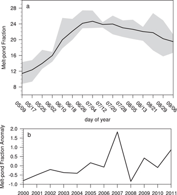
Figure 1. Variability of the MODIS melt pond fraction in the Arctic. (a) The evolution of the average fraction of sea ice area that is covered by melt ponds for the period 2000–2011. The gray area is the range of the melt pond fraction for the 12 year period. (b) Time series of the pond fraction anomaly (the average from 9 May to 6 September).
Download figure:
Standard image High-resolution imageA significant increasing trend in the melt pond fraction is observed during 2000–2011, which is superimposed on the strong interannual variability (figure 1(b)). The year 2007 (the lowest September ice extent during 2000–2011) had the largest melt pond coverage in late July, reaching ∼30–40% in the Northern Beaufort, Chukchi and Northern East Siberian Seas, the Central Arctic Basin, the Canadian Archipelago and the Northern Greenland Sea (not shown).
To examine the association between the melt pond fraction and sea ice extent, we compute the correlation between the time series of the observed pond fraction and September ice extent during 2000–2011. Care is needed when assessing correlation between two variables that have significant trends. It is possible that two variables linked statistically are physically independent in reality. To address this issue, here we focus on the detrended time series. We integrate the pond fraction over time and space to obtain the time series of melt ponds [20, 25]. Temporally, we integrate the pond fraction varying from 9 to 17 May, 9 to 25 May, and up through 9 May to 6 September. Spatially, we calculate the correlation coefficient between the detrended time series of the above integrated pond fraction at each grid point and the detrended time series of the ice extent in September. More spring and summer melt ponds result in less sea ice the following September; thus, melt ponds and September sea ice extent are negatively correlated. The resulting correlation maps demonstrate the spatial distribution of the strength of correlations between the pond fraction and September ice extent. As shown in figure 2 and in contrast to S14, in the observational data only scattered significant negative correlations are found in the Arctic as the pond fraction is integrated through May only (as well as early June) only (figure 2(a)). By contrast, significant negative correlations form large spatial clusters centered in the Northern Beaufort and Chukchi Seas when the pond fraction is integrated to mid-June. In late June, the areas with significant negative correlations become broader, covering the Northern Beaufort and Chukchi Seas, the Central Arctic Basin, the Canadian Arctic, and the Northern Greenland Sea (figure 2(b)). Extending the integration time period beyond late June yields only minimal change in the areas of significant negative correlations (figure 2(c)).
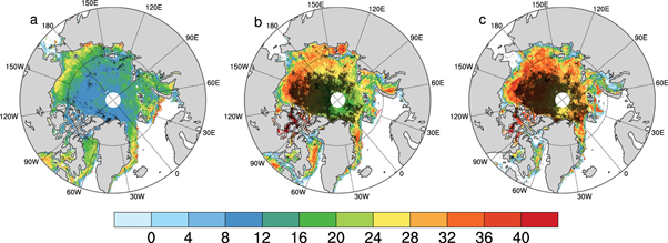
Figure 2. Distribution of the MODIS melt pond fraction from 9 May to the day given. (a) 2 June, (b) 26 June, and (c) 20 July. Color is the averaged pond fraction for the day given during 2000–2011. The dark gray dots are the statistically significant correlations between the pond fraction integrated from 9 May to the day given and September Arctic sea ice extent.
Download figure:
Standard image High-resolution imageFor the grid points with a significant negative correlation coefficient between the pond fraction and September ice extent (gray dots in figure 2(b)), we calculate the correlation between the pond fraction integrated varying from 9 to 17 May, 9 to 25 May, up through 9 May to 6 September. In contrast to the modeling results in S14, which showed that the pond fraction in May has the strongest impact on the ice extent in the coming September (r = −0.8), satellite observations show there is no significant correlation between the pond fraction in May and September ice extent (r > 0). Moreover, the integrated pond fraction from May to early June shows no or weak correlation (not statistically significant) with the ice extent in September. A highly significant correlation (r = −0.8, > 99% significance) between the pond fraction and September ice extent is first observed when the melt pond is integrated from May to late June. Hence the timing of the strong relationship is about one month later than those found in S14. Furthermore, we note that the high correlation achieved in late June does not persist through July (figure 3). The correlation degrades from early to mid-July, and then the highly significant correlation recovers in late July. After that, extending the integration time period does not improve the correlation, which by then has reached 0.9.

Figure 3. Correlation between time series of the melt pond fraction (integrated from 9 May to the day given) and September Arctic sea ice extent. The horizontal gray lines are the 95% (dashed) and 99% (solid) confidence levels.
Download figure:
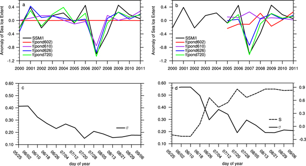
Standard image High-resolution imageTo examine the potential of the melt pond fraction as an indicator for the September sea ice extent, following S14, we apply linear regression to reproduce the September ice extent (Ysie) using the pond fraction (Xmpf) as the predictor. The regression model can be expressed as: Ysie = A + BXmpf + e, where A and B are determined by the least squares approach and e is the model residual. We use linear regression to calculate the September ice extent from the pond fraction integrated varying from 9 to 17 May, 9 to 25 May, up through 9 May to 6 September during 2000–2011. Clearly, the September ice extent predicted based on the pond fraction in May cannot capture the observed year-to-year variability (figure 4(a)). By contrast, the observed interannual variability is well reproduced as the pond fraction is integrated through late June, and especially as the pond fraction is integrated through late July. As shown in figure 4(c), the regression error (root mean square error) decreases significantly from May to mid-June, reaching 0.23 million km2 in late June. The lowest regression error, which is achieved in late July (0.15 million km2), is a factor of three smaller than the standard deviation of observed September ice extent during 2000–2011.
Figure 4. Regressed and predicted September Arctic sea ice extent anomaly (detrended). (a) Regressed ice extent anomalies for three different integration periods (2 June, 10 June, 26 June, and 20 July) and (c) their regression errors. (b) Predicted ice extent anomalies and (d) their predicted errors (left y-axis label) and forecast skills (right y-axis label).
Download figure:
Standard image High-resolution image
The above linear regression uses all the data during 2000–2011 to train the coefficients in the linear regression model. For the forecast, only data from previous years is used. Following S14, data only from the first five years are used to calculate the coefficients of the linear regression model as well as the error for the forecast years (2005–2011). The forecast skill can be expressed as:  where
where  is the standard deviation of the forecast error and
  is the standard deviation of the detrended observed September ice extent (0.51 million km2 for 2005–2011). In general, the errors of the predicted September ice extent for the forecast are larger than those of the above 2000–2011 regression. Similarly to the regression results, the predicted September ice extent based on the pond fraction in May deviates from the observation by large margins, i.e. the forecast errors for some years are larger than
  (figure 4(b)). By contrast, as the pond fraction is integrated to late June, the predicted ice extent is close to the observations, especially as the pond fraction is integrated to late July. As shown in figure 4(d), the forecast skill increases significantly from late May (no skill) to late June (0.66). The opposite is the case for the forecast error. The highest forecast skill is achieved in late July (0.86), with the smallest forecast error of 0.19 million km2. This forecast skill is remarkably higher than those reported in the SIO [6, 14].
Note that although the correlation between the pond fraction and September ice extent increases significantly from 2 to 10 June (figure 3) and the observed interannual variability of September ice extent can be reproduced to some extent as the pond fraction is integrated to 10 June (figure 4(a)), the regression error of 10 June is still much larger than that of 26 June (figure 4(c)). More importantly, the predicted September ice extent based on the pond fraction integrated to 10 June still deviates from the observation by large margins (figure 4(b)). By contrast, the predicted ice extent based on the pond fraction integrated to 26 June is close to the observations (figure 4(d)).
4. Discussion and conclusion
We conclude that the amount of melt pond fraction integrated from the beginning of the melt season to early-to-mid summer plays a critical role in determining the evolution of the sea ice state throughout the melt season, and promises to improve the prediction of how much sea ice will melt by the end of the melt season. However, we see no evidence of predictive skill in May as indicated in S14, and note that S14 estimates of the predictor variable (melt pond fraction) in May differ dramatically from the observations. Whereas model predictive skill is established by mid-May (reaching the highest by the end of May) and actually falls slightly for integrations extending into June, observed predictability is only established in late June, rising rapidly from zero skill in early-to-mid June. This suggests that the timing of melt pond formation is critical. Some studies have suggested that the persistence of Arctic sea ice extent anomalies is shorter during spring and longer during summer [26, 27], which may be part of the reason that integrations that span late June and July melt pond fraction are better predictors than those that only integrate through May.
Despite these important differences, in a broader sense our study is similar to S14 in that it does find predictability based on melt ponds. It should also be mentioned that our results do not necessarily indicate that the predictive skill of the model described in S14 is less than reported. Nevertheless, our findings (low predictive value of observed May melt ponds, and large bias in the amount of modeled May melt ponds) raise the possibility that something other than melt pond formation (such as perhaps surface melt onset and/or above freezing temperatures) could be the source of the model predictability. These findings point to the importance of reconciling model simulations and the observations. Given the limitations of current models, it is critical both that the observational record be extended, and that model diagnostics that could explain physical links between the evolution of melt ponds and sea ice conditions be reported for standardized comparison to observations. Without such reporting, it will be difficult to advance physical understanding of how early season melt ponds influence late season sea ice extent, or rule out other possible explanations such as overfitting or overparameterization in the model.
To date, the assumptions of sea ice optical physics made in the sea ice model component of climate forecast systems and global climate models are inadequate to properly represent melt ponds, i.e. the models that participated in the Climate Model Intercomparison Project phase 5 [28] do not have any—or have only simplistic—melt pond parameterizations. Furthermore, recent large-scale under sea ice light measurements from a remotely operated vehicle showed that the first-year ice that is extensively covered by melt ponds, not only allows three times more solar radiation to penetrate than multi-year ice allows, but also absorbs 50% more solar radiation than multi-year ice [29]. This indicates that current forecast systems and climate models might underestimate the melt pond induced albedo-transmission feedback, particularly as the Arctic sea ice entering a new regime of thinner and predominantly first-year ice. Thus, for operational forecasts of seasonal sea ice and climate projections of the ice-free Arctic [30, 31], climate forecast systems [32] and global climate models [28] that account for realistic melt ponds, especially their evolution from early spring to mid summer, seem to be a worthy area of expanded research and development.
Finally, it must be noted that the statistical forecasting methods based on historical relationships may not hold true in the future given that the Arctic climate is changing in ways without precedent for at least the past millennium [3, 33].
Acknowledgments
This research is supported by the NOAA Climate Observations and Monitoring Program (NA14OAR4310216) and the National Natural Science Foundation of China (41176169). The views expressed herein are those of the author(s) and do not necessarily reflect the views of NOAA.