
Abstract
Power production from wind turbines can deviate from the manufacturer's specifications due to variability in atmospheric inflow characteristics, including stability, wind shear and turbulence. The practice of insufficient data at many operational wind farms has made it difficult to characterize this meteorological forcing. In this study, nacelle wind measurements from a wind farm in the high plains of central North America were examined along with meteorological tower data to quantify the effects of atmospheric stability regimes in the boundary layer on turbine power generation. The wind power law coefficient and the bulk Richardson number were used to segregate time periods by stability to generate regime-dependent power curves. Results indicated underperformance during stable regimes and overperformance during convective regimes at moderate wind speeds (8–12 m s−1). Statistical testing using the Monte Carlo approach demonstrated that these results were robust, despite potential deviations of the nacelle wind speeds from free-stream inflow values due to momentum loss from the turbine structure and spinning rotor. A hypothetical stability dependence between free-stream and nacelle wind speeds was generated that can be evaluated in future analyses. The low instrumentation requirement of our power analysis technique should enable similar studies at many wind sites formerly considered inappropriate.
Export citation and abstract BibTeX RIS

Content from this work may be used under the terms of the Creative Commons Attribution-NonCommercial-ShareAlike 3.0 licence. Any further distribution of this work must maintain attribution to the author(s) and the title of the work, journal citation and DOI.
1. Introduction
Global wind power production has grown rapidly over the past decade in response to supply uncertainties, geopolitical instabilities, and climate threats posed by dependence on fossil fuels. The global wind market experienced cumulative installed capacity growth of more than 20% in 2011 (GWEC 2011). To sustain this growth in the face of political and economic uncertainty and falling natural gas prices, improvement in wind turbine power yield is required to ensure wind remains an attractive option for new energy construction.
Two characteristics of the turbine inflow, wind shear and turbulence, both connected to the stability of the boundary layer, can significantly modify power output at wind farms. Theoretical analysis suggests that convective turbulence decreases performance in the concave portion of the power curve and increases performance in the convex portion (Kaiser et al 2007). Comparison of theory with observed atmospheric impacts on power production requires means to characterize the state of the turbine inflow. The following quantities have been used to classify inflow conditions: power law-wind shear exponents (Hunter et al 2001, van den Berg 2008 and Wharton and Lundquist 2012a, 2012b); horizontal turbulence intensity, i.e., the normalized standard deviation of the wind speed (Elliott and Cadogan 1990, Hunter et al 2001, Sumner and Masson 2006, Antoniou et al 2009, Rareshide et al 2009, and Wharton and Lundquist 2012a, 2012b); and vertical turbulence; the Obukhov length; and turbulent kinetic energy (Wharton and Lundquist 2012a, 2012b). Despite using different metrics, each study yielded a similar conclusion: variations in the atmospheric stability of the inflow can result in turbine power production that diverges from that estimated in the manufacturer's power curve (MPC), which correlates wind speed to expected turbine power output and is typically based on assumptions of neutral stability and, thus, only mechanical turbulence (IEC 61400-12-1 2003).
The stability of the atmospheric boundary layer over land is often non-neutral due to strong surface forcing driven by the daily cycle of solar heating. Resulting variability often leads to unexpected turbine power output as changes in wind shear and turbulence across the rotor-disk are not anticipated by the MPC. The correlation between boundary layer stability and power output varies among studies and the observation sites of focus. Elliott and Cadogan (1990) found decreased turbine performance during stable regimes, while Wharton and Lundquist (2012b) noted convective underperformance at moderate wind speeds. Rareshide et al (2009) observed that when wind shear was low, high turbulence led to higher turbine performance at low wind speeds, and lower performance at higher wind speeds, relative to low turbulence values. They also found that at low levels of turbulence, high shear values produced overperformance compared to lower shear values. Low wind shear and high turbulence values are more common in convective boundary layers, and the opposite is true in stable boundary layers. The inconsistent results of the previous studies indicate potential dependence of stability-power correlations on site-specific factors.
It is clear that more studies are needed to either uncover a general pattern of atmospheric influence on turbine performance or to characterize the multitude of different possible impacts, particularly as upward trends in hub height and rotor diameter subject turbines to wider variations of inflow shear, veer and turbulence (Larsen et al 2007). Unfortunately, many operational wind farms lack the meteorological observation platforms necessary to perform inflow analyses. Much of the existing literature was the product of enhanced instrumentation (e.g., remote sensing platforms) or the utilization of wind turbine test facilities which are inherently data-rich. Subsequently, some researchers have investigated the applicability of operational nacelle wind data towards inflow research. An obstacle to such research is the modification of nacelle-sampled flow by the turbine structure and rotor circulation, which can cause these measurements to nonlinearly deviate from free-stream values (Antoniou and Pedersen 1997, Smith et al 2002, Smaïli and Masson 2004). Nacelle transfer functions (NTFs), relationships between the nacelle-measured winds and free-stream winds, can be used to prepare nacelle data for use in power output studies, provided that conditions on the data collection platforms are met (Liu 2011). Modeling has also been used to calculate NTFs, though only for conditions of neutral stability (Keck 2012). Kankiewicz et al (2010) show that even when a transfer function cannot be derived, averaged nacelle measurements can provide precise and reasonably accurate depictions of wind farm inflow.
In this study, we use nacelle anemometry to investigate the relationship between turbine power production and atmospheric stability at a central North American high plains wind farm that features a typical suite of measurement platforms. To our knowledge, this is the first study to determine the statistical robustness of using nacelle winds to develop regime-dependent power curves. We demonstrate that statistically significant trends can be measured despite the potential deficiencies of nacelle anemometry.
2. Data collection and processing
2.1. Wind farm features and instrumentation
Data were collected at a wind farm located in the high plains of central North America, east of the Rocky Mountains. Terrain features across the wind farm were subtle, with a total elevation change across the farm not exceeding 80 m. A shallow drainage was centered approximately 20 km southeast of the wind farm. Figure 1 illustrates local terrain features and the location of data sources used. The land type within a 20 km radius of the wind farm was homogeneous and characterized by the United States Geological Survey as mixed cropland/grassland. The wind farm consisted of 134 pitch-regulated, three-blade wind turbines. The turbines had hub heights and rotor diameters of approximately 80 m. Point wind measurements were taken by a cup anemometer on the nacelle. The nacelle wind speed and turbine power generation measurements were provided by the wind farm operator as 15 min averages.
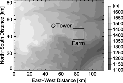
Figure 1. Relative locations of measurement platforms. The farm is located within the large box. The diamond represents the 60 m meteorological tower. Terrain contours are shown in meters above sea level for every 50 m.
Download figure:
Standard imageA 60 m tall meteorological tower was situated approximately 30 km from the wind farm, also located in cropland/grassland. This tower provided measurements of atmospheric pressure at a 1 m height above ground level (AGL) from a Vaisala PTB16 barometer, 10 and 60 m measurements of wind speed and direction using a Vaisala WM 52 ultrasonic anemometer, and air temperature and humidity from a Vaisala HMP 151 interferometer. Winds at 10 m recorded by the tower were compared to 10 m wind observations made on the northwest edge of the wind farm. The diurnally averaged 10 m wind speeds of the two observation platforms did not differ by more than 5%; this result suggests that the 60 m tower measurements typically represented meteorology similar to that of the farm 30 km away. Northwest and southeast were the dominant observed wind directions at this location at both 10 and 60 m. On-site precipitation measurements were not available. Therefore, relative humidity data were used as a proxy to identify possible precipitation events. All meteorological data were measured at 1 min resolution, which was insufficient for the computation of turbulence intensity. The data were averaged into 15 min intervals to match the turbine data.
Measurements spanned the springtime months of April and May 2010. The diurnal cycle dominated both the temperature and wind patterns during that time. Superimposed on this diurnal cycle were four synoptic frontal passages, with min-to-max differences in temperature of ∼ 30 °C. Accompanying these frontal passages were changes in both wind speed and direction. The relative rarity of frontal activity suggested that tower measurements were representative of wind farm conditions, as other propagating features that could cause spatial inaccuracy, such as drainage flows, do not typically reach rotor level.
2.2. Data filtering including the removal of wake effects
Initial data processing included removing time periods during which non-meteorological phenomena influenced power production, such as curtailments initiated by the power grid balancing authority (Fink et al 2009 and Rogers et al 2010). Reports of negative power generation values were flagged and removed. Observations from an Automated Surface Observing Systems (ASOS) station located ∼ 30 km from the farm, radar images and the farm relative humidity measurements were used in conjunction to identify periods with broad synoptic precipitation patterns. Two periods in which precipitation events strongly impacted power output were removed from the dataset, as the effects of rain and snow on turbine performance were not the focus of this study. In total, approximately 3.6% of the collected data were discarded in the aforementioned filtering operations.
Turbine wakes, the regions downwind of a turbine with reduced wind speeds, can also obfuscate the stability signal in power production. Therefore, wind direction sectors were flagged and removed for each individual turbine when an obstruction was sufficiently close, within 20 rotor diameters (20D), to potentially influence that turbine's inflow, as per IEC standard 61400-12-1 (2003). This location-based criterion is consistent with the work of Meyers and Meneveau (2011), who found that a turbine spacing of at least ∼ 15D downwind can minimize wake effects.
3. Defining stability bins for power curve analysis
In order to generate condition-dependent power curves, some quantity must be used to segregate wind power data into unique bins. Known relationships with wind shear and the diurnal evolution of the boundary layer make atmospheric stability a logical choice for characterizing turbine inflow. Many metrics exist for defining stability that range in complexity and the number of different measurements required. Here, stability bins are defined that are bounded by two different metrics: the wind speed power law coefficient (α) and the bulk Richardson number (RB).
The wind speed profile power law is used to describe the vertical change in wind speed with height. It is defined by the difference between the wind speed at two separate heights and the power law coefficient α, which can be derived empirically or used as a tuning parameter:
where U denotes the magnitude of the wind speed vector and z the corresponding height at which the wind measurement was made. In this study, the two heights used are 10 m and 60 m. Thus, when using the power law, nacelle wind measurements alone are insufficient because two different measurement heights are required. It is important to note that the power law coefficient is not intrinsically a measure of stability but instead is driven by stability. Other weaknesses of the power law coefficient include the inability to account for directional shear and the lack of theoretical basis (Justus and Mikhail 1976, Peterson and Hennessey 1977, Sisterson et al 1983, Walter et al 2009). Despite these shortcomings, the power law is commonly used in the wind industry, where a neutral value of 1/7th is typically assumed for α. It is utilized in this study because the data required to derive α values are often available at operational wind farms.
Access to both bulk-layer wind and temperature data allows for the computation of a traditional stability metric, the bulk Richardson number. This quantity is used to assess the impact on turbulent kinetic energy from buoyant production or destruction and kinetic (shear) production (Stull 1988):
where g is gravity, Δθv is the top-to-bottom difference in virtual potential temperature, Δz is the difference in height between measurements,  is the mean layer virtual potential temperature, and Δu and Δv are the top-to-bottom differences in wind speeds. As in the calculation of α, all differentials use 10 and 60 m data. Because of the lack of 60 m pressure data, extrapolation of 1 m surface pressures to 10 and 60 m was required for the calculation of potential temperature.
As a basic check on these calculations, day (7 AM–7 PM LT, or local time at the farm) and night (7 PM–7 AM LT) distributions of both α and RB (figures 2(a) and (b) respectively) were compared with the diurnal cycle. These histograms demonstrate that both stability parameters were consistent with typical boundary layer diurnal evolution over land. The day and night α values indicate that shear was, on average, higher during the night, similar to results documented by Kelley et al (2006) and Walter et al (2009) in other parts of the central plains of North America. During the day, large eddies homogenize the boundary layer, while at night, levels above the ground can become decoupled from surface influences, resulting in larger shear values (Blackadar 1957). RB was mostly negative during the day and typically ranges from −0.5 to 0.5 at night. In this case, buoyant air generates turbulent motions during the day, while at night buoyancy tends to suppress turbulence while the shear turbulence production term can become large (Stull 1988). A consequence of using data from the meteorological tower (10–60 m) is that the stability metrics defined above do not characterize directly the rotor-layer (40–120 m) but instead act as a proxy for rotor-layer variability. It is expected that measured quantities better match inferred values during the well-mixed daytime hours.
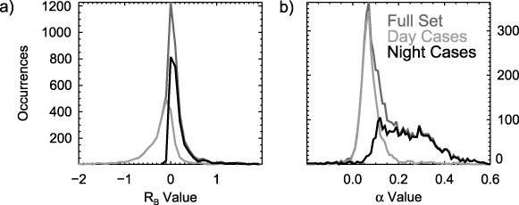
Figure 2. Full, day (7 AM–7 PM LT), and night (7 PM–7 AM LT) distributions of (a) RB and (b) α values. Bin sizes of 0.1 and 0.01 were used for RB and α respectively.
Download figure:
Standard imageValues of α and RB were compared to determine stability classifications (shown in figure 3). Three classes were defined based upon the shape and slope of the scatter relationship in figure 3 and references to values used in Wharton and Lundquist (2012b). The stable-to-neutral and neutral-to-convective delineations were estimated at α = 0.2,RB = 0.06 and α = 0.09,RB =− 0.17 respectively, which is a slightly wider range of neutral coefficient values compared to α = 0.2 and 0.1 in Wharton and Lundquist (2012b). The minor range differences were likely the result of site-specific factors such as land characteristics, height of observation, and relative dominance of the local synoptic regime. The chosen stability classes are compared in table 1. A time period was only classified as stable, neutral or convective if both parameters were consistent, which occurred in approximately 67% of the data. Opposite categorizations were found in 5.6% of all cases—these cases were classified as stable by RB and convective by α. The use of two stability criteria in defining bins emphasized the differences between stable and convective effects on inflow, which was a focus of this study. Such filtering operations would be less appropriate in wind farm site analyses, for which the entire range of conditions should be sampled.
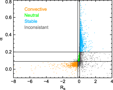
Figure 3. Visual representation of the relationship between α and RB for all time periods. Stable, neutral, and convective class delineations are indicated by the solid lines for each stability parameter.
Download figure:
Standard imageTable 1. The number of valid 15 min periods in each coupled stability classification. Bolded values indicate times for which both α and RB agree.
| RB stable | RB neutral | RB conv | Total | |
|---|---|---|---|---|
| α stable | 1398 | 67 | 0 | 1465 |
| α neutral | 614 | 760 | 41 | 1415 |
| α conv | 258 | 530 | 913 | 1701 |
| Total | 2270 | 1357 | 954 | 4581 |
4. Power output segregated by the combined α–RB stability metric
4.1. Power curve analysis
The effect of atmospheric stability on farm power production was illustrated through the creation of stability-segregated power curves using nacelle wind observations. These power curves were generated using an 'average farm turbine' approach in which data from all of the non-filtered turbines were combined to form power curves representative of an average turbine at the wind farm. One stability value derived from the meteorological tower was compared to 134 nacelle wind and turbine power output measurements for each time period; all times were then compiled for the two months to generate the relationships. Power curves were generated for stable, neutral, and convective conditions. The power curves based on stability segregation for all non-flagged turbines in the farm are shown in figure 4. In figure 4(a), a standard power curve is shown, while figure 4(b) provides the anomaly of the measured power output compared to neutral conditions. This second visualization emphasizes the differences between power production during neutral conditions typically assumed by the wind industry and that actually measured across a variety of conditions at an operational wind farm. Filled data points denote statistically distinct curves as determined using the rank-sum test with a 0.01 significance level; open data points are not distinct. The error bars indicate the median absolute deviation. This error metric was chosen because it minimizes the effect of outliers.

Figure 4. (a) Standard and (b) anomaly power curves for convective, neutral and stable classes. Error bars depict the median absolute deviation. In (b), the green horizontal line represents neutral conditions, and orange and blue lines represent the convective and stable anomaly (kW) from the neutral condition at a given wind speed. Filled circles are statistically distinct. Nacelle winds are binned in 0.5 m s−1 intervals.
Download figure:
Standard imageIn general, convective conditions exhibited a statistically significant performance advantage over stable conditions when inflow wind speeds ranged from 4 to 12 m s−1. The largest difference between the two inflow conditions (curve separation) occurred at 10.25 m s−1, for which average turbine power production was 87 kW higher during convective conditions compared to stable conditions. Analysis of the improvements realized by incorporating RB into the stability metric was conducted by comparing the 87 kW α–RB curve separation to that calculated only through the use of the power law coefficient. When only using α, the separation between convective and stable performance at 10.25 m s −1 decreases by 16 kW–71 kW.
The results presented in figure 4, which show general convective overperformance, agree with Elliott and Cadogan (1990) but disagree with those of Rareshide et al (2009) and Wharton and Lundquist (2012a, 2012b). Only Rareshide et al found results that agreed with the theoretical result of Kaiser et al (2007). This fact indicates that other site-specific complicating factors, such as atypical rotor-disk shear profiles, directional shears, and terrain effects, could be influencing results at other locations. The presence of low-level jets (LLJ), wind maxima that form as the boundary layer decouples from the surface due to nighttime cooling (Blackadar 1957), may influence the relative performance of turbines in stable periods compared to convective periods. An investigation into LLJ impacts would necessitate measurements from the top half of the rotor-disk, which were not available at this wind farm.
4.2. Are power trends based on nacelle winds valid?
As mentioned in the introduction, nacelle wind measurements do not sample the free-stream inflow as the turbine structure and rotor alter the flow in the process of removing momentum for power generation. Therefore, the stability trends described previously require validation to ensure that they are robust despite the use of nacelle wind measurements. Data sufficient to create a nacelle transfer function were not available in this study, so alternate means were required to evaluate the validity of the stability-based trends. The meteorological tower was too distant from the farm to successfully extrapolate the 60 m tower winds to those sampled at the 80 m turbine hubs. Therefore, the robustness of the nacelle measurements had to be determined using only the nacelle data; in this study we used the Monte Carlo statistical method.
In our Monte Carlo simulations, we isolated the largest α–RB stability class power curve separation: the 87 kW power anomaly difference between convective and stable classifications at 10.25 m s−1. Hypothetical systematic errors, created using a 5th-order polynomial fit of free-stream tower and nacelle data collected by Antoniou and Pedersen (1997) (shown in figure 5), and random errors, up to 1 m s−1 at any given time, were superimposed onto the nacelle wind measurements to simulate the expected range of errors caused by the use of nacelle observations. Then the data were processed into the previously derived stability bins and the difference between the two classes at 10.25 m s−1 was calculated and evaluated for significance at the 0.01 level using the rank-sum test. This process of adding noise and systematic error was repeated 1000 times with unique random errors generated in each iteration.
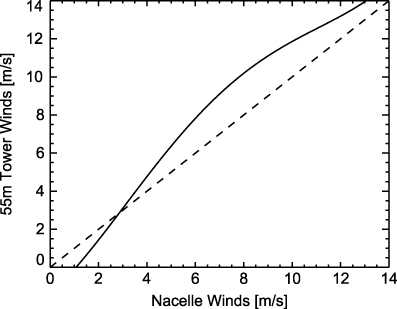
Figure 5. The solid line shows a hypothetical relationship between free-stream winds and nacelle anemometer-measured winds. The dashed line represents a 1:1 line. Adapted using 5th-order polynomial fit of data collected by Antoniou and Pedersen (1997).
Download figure:
Standard imageOn average, the effect of random errors was minimal while systematic errors reduced the power output difference between the convective and stable regimes from 87 to 50 kW. However, 100% of the 1000 simulations still produced statistically significant differences between the two classes. Furthermore, the observed pattern of convective regimes outperforming stable regimes was maintained. Thus, even with sizable systematic error, we find the nacelle measurements can be used in analysis of stability impacts on power curves.
An outstanding question remains: are the nacelle wind measurements themselves stability dependent? No studies of stability-dependent relationships could be found in the literature. Therefore, we have calculated stability corrections to the measured winds which would be necessary to adjust convective and stable power curves towards that of neutral flow. These hypothetical stability-dependent nacelle transfer functions are shown in figure 6. While the magnitudes of the corrections are within the range of previously observed values, neither the stable nor the convective correction matches the nacelle-free-stream relationships currently found in the literature (such as the pattern depicted in figure 5). Additionally, the nacelle anemometer can only be influenced by turbulence while the turbine rotor can be influenced by turbulence and the wind shear profile across the rotor. Therefore, we expect that differences in the systematic bias between free-stream and nacelle winds caused by stability variations are smaller than the manifestations of stability forcing in the wind power relationship. However, further study is required to evaluate that hypothesis, using data where both inflow measurements and nacelle observations are available.
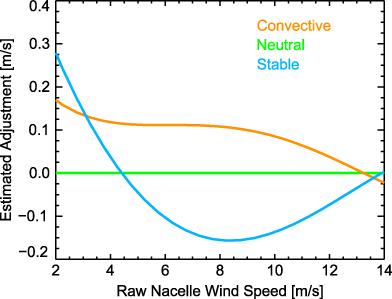
Figure 6. The estimated adjustments (m s−1) to convective and stable data for each raw nacelle-measured wind speed (m s−1) that would be required to eliminate stability dependence in the observed power data.
Download figure:
Standard image5. Summary and conclusions
An analysis was performed to investigate the relationship between power generation and meteorological conditions at a wind farm in the plains of central North America. Boundary layer stability, estimated using the wind shear parameter α and the bulk Richardson number RB, was used in conjunction with nacelle anemometry to determine inflow-power generation relationships. At low wind speeds below 8 m s−1, convective conditions common during the day tended towards higher power production than stable conditions common during the night. For moderate wind speeds in the range of 8–12 m s−1, this trend of higher performance during convective conditions reached a maximum. At high wind speeds above 12 m s−1, stable conditions resulted in higher power output, but differences between convective and stable conditions were minor at those wind speeds. Significance testing using the Monte Carlo approach demonstrated that the nacelle wind measurements were robust in identifying boundary layer stability impacts on power performance.
These results suggest that improved forecasts of wind farm output could be produced if the stability of the boundary layer was also forecast with skill. However, a more thorough analysis with a higher level of confidence necessitates turbine-independent measurements across the area swept by the rotor-disk. Remote sensing instruments such as LIDAR (Smith et al 2006, Courtney et al 2008, Aitken et al 2012 and others) or SODAR (Kelley et al 2007 and others) would improve understanding of how the evolution of wind shear in the rotor-disk affects power generation and the representativeness of the nacelle wind speed measurement. In lieu of additional data, we observed that stable, high shear conditions negatively impacted power production at moderate wind speeds at this farm, perhaps because of changing wind direction with height or atypical shear profiles at this location. The fact that we could generate these results using common tower and hub height measurements demonstrates that improvements in forecasting wind farm performance and site prospecting (through understanding the potential for over or underperformance due to local stability) are possible using relatively inexpensive technologies. In particular, the larger power curve separation obtained by adding RB, a traditional stability metric, underscores the need to have at least two temperature measurements at separate heights.
Our results agree with a portion of the prior literature while disagreeing with others; the lack of consistent meteorological forcing across farms indicates site-specific influences. Additionally, this analysis was performed during the spring months at a location that experiences different climatic conditions during each season. Future investigations should test these conclusions using longer datasets, potentially at multiple sites, in order to obtain a full record of turbine power output stability dependence. Ultimately, the success in using nacelle winds to perform this and other analyses should enable similar studies at sites previously considered inappropriate with the eventual goal being a comprehensive catalog of the varied meteorological forcings on wind turbine power production.
Acknowledgments
This study was funded by the National Center for Atmospheric Research (NCAR) under subcontract Z10-86199, and was made possible through the data contributions of the utility company. The authors would like to thank Sue Haupt, Bill Mahoney, Gerry Weiner, Neil Kelley and Sonia Wharton for several useful contributions to this research. We would also like to acknowledge the valuable comments and suggestions provided by our reviewers.