
Abstract
We investigate future changes in the annual cycle of heavy daily precipitation events across the British Isles in the periods 2021–2060 and 2061–2100, relative to present day climate. Twelve combinations of regional and global climate models forced with the A1B scenario are used. The annual cycle is modelled as an inhomogeneous Poisson process with sinusoidal models for location and scale parameters of the generalized extreme value distribution. Although the peak times of the annual cycle vary considerably between projections for the 2061–2100 period, a robust shift towards later peak times is found for the south-east, while in the north-west there is evidence for a shift towards earlier peak times. In the remaining parts of the British Isles no changes in the peak times are projected. For 2021–2060 this signal is weak. The annual cycle's relative amplitude shows no robust signal, where differences in projected changes are dominated by global climate model differences. The relative contribution of anthropogenic forcing and internal climate variability to changes in the relative amplitude cannot be identified with the available ensemble. The results might be relevant for the development of adequate risk-reduction strategies, for insurance companies and for the management and planning of water resources.
Export citation and abstract BibTeX RIS

Content from this work may be used under the terms of the Creative Commons Attribution-NonCommercial-ShareAlike 3.0 licence. Any further distribution of this work must maintain attribution to the author(s) and the title of the work, journal citation and DOI.
1. Introduction
Extreme precipitation often has great impacts on water management, agriculture and infrastructure (IPCC 2012). In particular the occurrence and severity of flood hazards are affected by various characteristics of precipitation, such as intensity, duration, amount, timing and phase (rain or snow) (IPCC 2012). Changes in the hazard frequency and occurrence during the year will have a strong impact on the ability of societies and ecosystems to cope and adapt to these changes (IPCC 2012). Thus, knowledge of future changes in the timing of extreme precipitation is necessary for the development of adequate risk-reduction strategies, for insurance companies and for the management and planning of water resources (IPCC 2012, and references therein).
Over the British Isles, observed 1961–2006 winter (summer) total precipitation have been shown to increase (decrease or be stationary) (Osborn and Hulme 2002, Fowler and Kilsby 2003a, Maraun et al 2008). For the last decades of the 20th century, seasonally and regionally varying changes in the intensity of heavy precipitation events have also been observed (Fowler and Kilsby 2003b, Maraun et al 2008, Jones et al 2012): spring and autumn heavy precipitation show the strongest increase (across the UK), winter extremes an increase (across most regions), while summer heavy precipitation shows a significant decrease in intensities (most prominent in the south and east of the UK) (Fowler and Kilsby 2003b). For southern regions of the UK, changes from summer peak rainfall to autumn peak rainfall have also been observed during the last decade of the 20th century, while no change in western regions could be detected (Fowler and Kilsby 2003b).
For Europe, an increase of extreme precipitation intensities is projected for the north and a decrease for the south (Buonomo et al 2007, Beniston et al 2007, Fowler et al 2007, Christensen et al 2007, Maraun 2012). Changes in the simulated intensity of annual and seasonal precipitation extremes for the UK have been studied for instance by Ekström et al (2005), Fowler and Ekström (2009), Fowler et al (2010), Huntingford et al (2003) and Buonomo et al (2007): for most British regions an increase in heavy precipitation intensities at the end of the 21st century is projected for spring, winter and autumn. For summer an increase is projected for some regions (e.g., Scotland (Maraun 2012)), while for other regions no clear signal has been found (Fowler et al 2010, Maraun 2012). Where robust long term trends have been identified in the observations for the UK, e.g., for Scotland in winter, projected trends are in keeping with those observed.
The large-scale patterns of these changes are generally robust to Regional Climate Model (RCM) formulations for Europe (Buonomo et al 2007). Also the seasonal fractions and intensities of extreme precipitation are consistent between RCMs, although the response of the seasonal intensities is noisy (Buonomo et al 2007).
For the UK, Maraun et al (2012) showed that the relationship between heavy precipitation and synoptic airflow is well represented in RCMs. Furthermore it has been shown that the peak times of the annual cycle of extreme precipitation are well modelled by most RCMs, whereas the representation of its amplitude shows deficits (Schindler et al 2012).
In this study we investigate future changes in the annual cycle of heavy precipitation over the British Isles, as projected by twelve climate model simulations for the periods 2021–2060 and 2061–2100. Changes in the annual cycle's peak times and relative amplitudes (i.e., amplitude relative to the average annual extreme) are analysed with respect to the consistency of the climate model simulations (and their coherence with observations).
2. Data
The transient scenario simulations of the 1951–2100 period are provided by the ENSEMBLES project (Van der Linden and Mitchell 2009). We use twelve precipitation data sets of eight RCMs with lateral boundary conditions from six high-resolution, Atmosphere–Ocean General Circulation Models (AOGCMs) (table 1). The integrations of the AOGCMs were forced with the IPCC SRES A1B scenario. The RCMs used in this study operate on a rotated pole grid with approximately 25 km horizontal grid spacing. We restrict the analysis to the domain of the British Isles (2°E–10°W, 50°–60°N).
Table 1. List of RCMs with driving AOGCMs considered in this study. The acronym of the institute is given in brackets.
| RCM | Driving AOGCM |
|---|---|
| HadRM3 Q0 (HC) | HadCM3 Q0 (HC) |
| HadRM3 Q3 (HC) | HadCM3 Q3 (HC) |
| HadRM3 Q16 (HC) | HadCM3 Q16 (HC) |
| HIRHAM5 (DMI) | ARPEGE (CNRM) |
| BCM (NERSC) | |
| ECHAM5 (MPI-M) | |
| RACMO2 (KNMI) | ECHAM5 (MPI-M) |
| REMO (MPI-M) | ECHAM5 (MPI-M) |
| RCA (SMHI) | BCM (NERSC) |
| ECHAM5 (MPI-M) | |
| HadCM3 Q3 (HC) | |
| RCA3 (C4I) | HadCM3 Q16 (HC) |
For the Hadley Centre models the ENSEMBLES project provides runs with three parametrizations resulting in different climate sensitivities Q0 (standard), Q3 (low) and Q16 (high) (Collins et al 2006).
For the analysis of possible changes in the peak times of the annual cycle, we select three 40 yr time slices: 1961–2000 (present day), 2021–2060 (mid future) and 2061–2100 (far future).
3. Methods and concepts
3.1. Statistical model
We model the annual cycle of heavy precipitation as an inhomogeneous Poisson process with a non-stationary threshold, for details see Coles (2001). Therefore we assume that the intensities of rare, heavy precipitation events can be described by the generalized Pareto distribution (Davison and Smith 1990) and that their occurrences are Poisson distributed and independent (to adapt the model to dependent data, the standard errors of the maximum likelihood estimates are adjusted (Fawcett and Walshaw 2007, and references therein)). To easily include the annual cycle via sinusoidal models for the location and the scale parameters the model has been reparametrized in terms of the generalized extreme value (GEV) distribution. This model has been shown to describe the annual cycle of heavy precipitation properly throughout the United Kingdom (Rust et al 2009, Maraun et al 2009). A short description of the statistical model, the choice of the threshold and the goodness-of-fit criterion is provided in section A.1, for details on the methods see Schindler et al (2012). The result of the goodness-of-fit analysis is given in the supplementary online material (SOM; available at stacks.iop.org/ERL/7/044029/mmedia).
3.2. The annual cycle of heavy precipitation and its change
The annual cycle is defined by the monthly return levels, zp(m), for each month m of the year, defined as the value which is exceeded in month m with a probability p, e.g., z0.04(Jan) (see section A.2). This corresponds to the 25 yr monthly return levels, which we will focus our analysis of the annual cycle on. The average over all 12 monthly return levels is denoted by  , defining an annual return level.
We define the peak time of the annual cycle of the monthly return levels as the month for which zp(m) is maximal, i.e., argmax(zp(m)). The amplitude is defined as half the range of the monthly return levels, zp(m). Since this value is only meaningful in relation to the average monthly return level, we define the relative amplitude as the ratio of the amplitude and the average monthly return level, i.e.,  . This relative value is comparable over regions with different magnitudes of monthly return levels.
All relevant characteristics of the annual cycle are summarized by the annual return level, peak time and relative amplitude. As annually and seasonally resolved changes of extreme precipitation across the UK are already well studied (Ekström et al 2005, Fowler and Ekström 2009, Fowler et al 2010, Buonomo et al 2007), we focus on peak times and relative amplitudes only. Schindler et al (2012) demonstrated that peak times are well represented by RCMs, but relative amplitudes are misrepresented for many regions. This insufficiency has to be kept in mind for the interpretation of any results related to the relative amplitudes.
In the situation of a very low relative amplitude, the peak time is not very robust and therefore also its change is not easily interpretable. The direction of change is defined as the sign of future minus reference peak times (relative amplitudes). A shift of the relative amplitude by more than 5% of the reference period's relative amplitude is considered a change.
4. Results and discussions
4.1. Change of the peak times
The multi-model mean of the simulated peak times of the reference time period (1961–2000) is plotted in figure 1. It shows the typical east–west gradient with earlier peak times in the east and later peak times along the west coast of Great Britain and Ireland. For the two future time periods the twelve climate simulations vary considerably in the projection of the peak times (see SOM). In the multi-model mean for both future time periods, earlier or non-changing peak times are projected for the north-western regions and later peak times for the south-eastern regions (figure 2). The biggest shift is almost two months later for the far future (figure 2, right). This south-west–north-east division is also visible in figure 3, showing the fraction of climate simulations which project the same direction of change. For the far future, the signal is relatively strong in the south-eastern region. More than half of the projections agree on a shift of the peak times of the annual cycle towards later times in the year (figure 3, right). This signal is disturbed by internal climate fluctuations and hardly emerges for the mid future (figure 3, left). The change in the peak times is mostly consistent over different time periods: most climate simulations project a smaller or no change to the mid future and a bigger (or equal) change in the same direction for the last 40 years of the 21st century (figure 3 and SOM).

Figure 1. Peak times of the reference period: multi-model mean of the twelve climate simulations for the period 1961–2000.
Download figure:
Standard image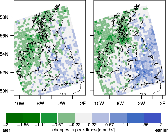
Figure 2. Changes in the peak times of the annual cycle: colour-coded is the multi-model mean of all simulated changes relative to 1961–2000; future period: left: 2021–2060, right: 2061–2100; green: changes to later times, blue: to earlier times.
Download figure:
Standard image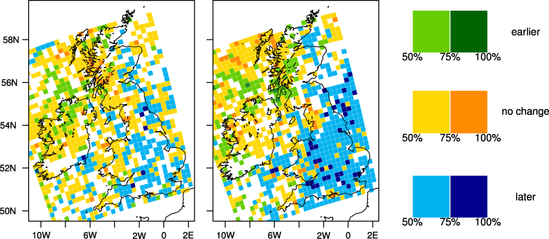
Figure 3. Changes in the peak times of the annual cycle: colour-coded is the percentage of climate simulations which agree on the same direction of change relative to 1961–2000; future period: left: 2021–2060, right: 2061–2100; yellow: no change, blue: change to later peak times, green: change to earlier peak times. Light colours: half of the climate projections agree, dark colours: more than 75% of the simulations agree on the same direction of change. White: no agreement (less than 50% of the simulations agree).
Download figure:
Standard imageThe difference between eastern and western regions becomes gradually less pronounced (smaller difference and lesser spatial extent) in the two future projections (see SOM). There is no clear contribution of the driving AOGCM or the downscaling RCM to the change signal (not shown). However, there is a tendency that the driving AOGCM dominates the pattern of the direction of change, while no systematic influence of the RCM becomes apparent (see SOM).
4.2. Change of the relative amplitude
The multi-model mean pattern of the relative amplitude over the reference period shows three distinct regions with high values (figure 4): at the west coast of Great Britain, in the west of Ireland and in eastern England, the monthly return levels vary with the season by at least 17% of the annual return level3 (up to 30% in Scotland). This pattern is similar to the one of the relative amplitude based on gridded observations (Schindler et al 2012). The direction of change depends strongly on the driving AOGCM (figure 5). ECHAM5-driven simulations project increasing relative amplitudes almost everywhere for both time periods (figure 5, left). HadCM3-driven simulations project decreases in southern and central England and increases for the far future everywhere else (figure 5, middle). A closer look at 31 arbitrary grid points4 located in England and Scotland (divided into four subregions) reveals remarkable differences (figure 6): for all grid points, ECHAM5-driven simulations show an upward trend, while ARPEGE- and BCM-driven simulations show mostly a negative signal; HadCM3-driven runs show greater variability and no common signal, even when subdivided by climate sensitivities. This behaviour depends on the driving AOGCM and to a lesser extent on the region (figure 6). Therefore also the common signal for the western regions (figure 5) might rather be due to internal climate fluctuations than due to anthropogenic forcing.
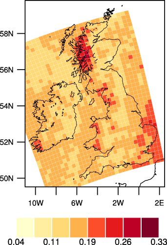
Figure 4. Relative amplitude of the reference period: multi-model mean of the twelve climate simulations for the period 1961–2000.
Download figure:
Standard image
Figure 5. Changes in the relative amplitude: colour-coded percentage of simulations 2061–2100 relative to reference period separated according to driving AOGCM (ECHAM5 (left), HadCM3 (middle), BCM/ARPEGE(right)). White: no agreement (less than 50% of the simulations agree).
Download figure:
Standard image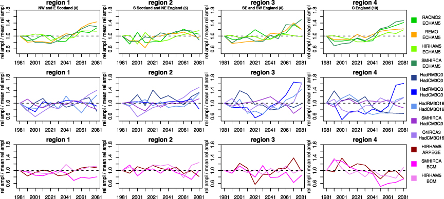
Figure 6. Temporal evolution of regional relative amplitude: estimated at 31 grid points, subdivided and averaged into 4 regions for eleven 40 yr time periods (centred on the year given on the x-axis). Colour-coded the RCM-AOGCM simulation. Top panel: ECHAM5-driven RCMs. Middle panel: HadCM3-driven RCMs. Bottom panel: BCM/ARPEGE-driven RCMs. Left panel (region 1): 8 north-west and east Scottish grid points. Left middle panel (region 2): 5 south Scottish and north-east English grid points. Right middle panel (region 3): 8 south-west English grid points. Right panel (region 4): 10 central English grid points.
Download figure:
Standard image4.3. Discussion
The change in peak times for the southern and eastern regions of the UK towards later peak times is coherent with findings for observations by Fowler and Kilsby (2003b). They proposed changes in the Scandinavian pattern in autumn and North-Atlantic Oscillation (NAO) in winter as sources of the observed changes in peak times from summer to autumn5. However in the present RCM ensemble we do not find evidence that the Scandinavian pattern causes the change in peak times for eastern England: the Scandinavian pattern is well represented in the CMIP3 simulations (Handorf and Dethloff 2009), but there is no consistent response of the Scandinavian pattern to increased greenhouse gas emissions between global circulation models (Haugen and Iversen 2008). The projected change in peak times from summer to autumn is consistent across the simulations studied. Therefore the Scandinavian pattern cannot explain the consistent shift in the modelled peak time patterns.
The pattern-based NAO index shows an increase (for both summer and winter) in most AOGCMs considered in this study6 but the magnitudes of the increase spreads considerably (Bladé et al 2012a, Karpechko 2010, Handorf and Dethloff 2009). The winter NAO primarily influences heavy precipitation in western regions of the British Isles (Maraun et al 2012, Haylock and Goodess 2004, Scaife et al 2008, Santos et al 2007). Thus the influence on the regions for which a response is consistent, i.e., eastern England, is small. Therefore the winter NAO might only explain a small portion of the observed shift in eastern England.
To explain the potential role of the summer NAO and the East Atlantic pattern for the consistent shift from summer to autumn peak times further research needs to be carried out. For monthly mean precipitation both the NAO and the East Atlantic pattern have already been shown to have a significant influence on summer precipitation throughout the British Isles (Murphy and Washington 2001, Bladé et al 2012b).
The changes in the relative amplitude of heavy precipitation for the middle and end of the 21st century for the western regions is coherent with already observed changes during the end of the 20th century (Fowler and Kilsby 2003b). The inter-AOGCM variability of the relative amplitude's response is larger than the inter-RCM variability7. ECHAM5-driven simulations show a positive trend, BCM/ARPEGE-driven simulations show a rather negative trend and HadCM3-driven simulations do not show a common signal. Thus either the relative amplitude is dominated by internal climate variability or at least two of the three AOGCMs do not correctly simulate the sign of future trends. To identify the contribution of internal variability and of uncertainties from driving AOGCMs, initial condition ensembles and a wider range of driving AOGCMs are needed.
The mechanisms describing the relative amplitude as well as the peak times of heavy precipitation need further investigation. For instance, it is not clear to what extent the Scandinavian, East Atlantic and other teleconnection patterns are of relevance for the relative amplitude of extremes. Both the Scandinavian pattern's and the East Atlantic pattern's representation in the CMIP3 AOGCMs vary considerably between climate models (Handorf and Dethloff 2009). This could be a starting point for explaining the dependence of the relative amplitude's change on the driving AOGCM.
5. Conclusions
We analyse projected changes in the annual cycle of extreme precipitation over the British Isles. The changes of the peak time, as well as its changes in the relative amplitude are shown and discussed. Changes in the peak times are robustly projected for the end of the century, whereas the signal in the next three decades is rather weak and disturbed by internal climate fluctuations.
The spatial patterns of this change varies considerably between AOGCM-RCM combinations. On a regional scale one should therefore interpret these regional results with care. The gradient in the peak times between eastern and western parts of the UK becomes weaker in the future: in the eastern parts of the UK the annual cycle is projected to peak later in the year while in the western parts—depending on the simulation—the peak times remain unchanged or are earlier in the year.
For the amplitude of the annual cycle, relative to the annual return level, there is an indication for an increase for some western regions. This change is noisy both in space and time. For the eastern regions the employed AOGCMs do not even agree on the sign of the projected response.
The changes in the peak times might imply a higher risk of flooding: for eastern regions, due to the shift in peak extreme rainfall from late summer to autumn, the peak time of intense rainfall will move closer to the high risk season. For western regions a shift from December to November peak times increases the likelihood of intense rainfall coinciding with a high risk situation already in current climate. For the identified regions and months, it might become necessary to install suitable adaptation measures towards the end of the century. In some regions of central and southern England this might become already necessary for the mid of the century.
Acknowledgments
Andrea Toreti and Juerg Luterbacher acknowledge support by the 7th EU-Framework programme ACQWA (#212250). The ENSEMBLES data used in this work was funded by the EU FP6 Integrated Project ENSEMBLES (contract number 505539) whose support is gratefully acknowledged. The analysis was carried out with software written in R (R Development Core Team 2011), based on the ismev package (Coles and Stephenson 2010) and evd package (Stephenson 2002). We thank the reviewers for their constructive criticism and helpful suggestions.
Appendix:
A.1. Statistical model and threshold selection
For readability we sketch the statistical model described by Schindler et al (2012). We model rare events as an inhomogeneous Poisson process which is characterized by its intensity measure on [0,1] × [z,∞], for z greater than a suitable threshold u:
where μ,σ and ξ are called location, scale and shape parameters. The intensity measure describes the probability of exceeding a level z.
These parameters are adjusted such that at each time t the annual cycle is accounted for:


Since the shape parameter is difficult to estimate with limited amount of data, it is kept constant (Rust et al 2009). Introducing additional (seasonally varying) parameters would lead to very uncertain estimates. For the realizations zi of the random variable Z, for i = 1,...,Nobs, where Nobs is the number of observations, one can estimate the parameters, (μ0,μ1,μ2,σ0,σ1,σ2,ξ)≕θ, by maximizing the likelihood function with respect to θ. In general it is easier to minimize the negative log-likelihood function than to maximize the likelihood function. With δi = 1 if zi > ui and δi = 0 else we hence obtain
with np being the number of observations per block and the non-stationarity of the parameters denoted as μi:=μ(ti) and σi:=σ(ti), ti∈{1,...,365.25 × 4} being the time of the observation zi in the 4 yr cycle.
To select rare events a high threshold u ≫ 1 is fixed, such that above it, the asymptotic marginal and dependence properties appear to be stable (Davison and Smith 1990). We select u by choosing the 95%-quantile of the anomalies with respect to the climatological mean over the 40 yr period as a threshold. We apply an automatic procedure to check the goodness-of-fit: we simulate a 95% confidence interval (CI) for the quantile–quantile plot and count the points outside the CI. If more than 5% of the threshold exceedances lie outside the CI, the fit is considered critical. If 5% or less of the grid points of one data set indicate a critical fit, this is considered statistically expected and the threshold is not changed. If there are more than 5% critical grid points in one data set, we increase the threshold by one per cent, refit the statistical model and start over again. The iteration halts if the threshold reaches the 97%-quantile, the remaining critical grid points are excluded from the subsequent analysis.
A.2. The annual cycle
The annual cycle of the monthly return levels is defined via the twelve monthly return levels. In this non-stationary setting the calculation of the return levels, zp, is an inverse problem (Coles 2001):

where
with the non-stationarity of the parameters denoted as μj:=μ(tj) and σj:=σ(tj) for j∈{1,...,np} and np being the number of observations per block. To calculate the annual return level zp the block length is set to 365, i.e., np = 365. To calculate monthly return levels, zp(m), (non-stationary setting) the product over the index set is restricted to a specific month, m. This can be achieved by choosing j∈{1,...,np} in (A.4) such that tj∈m (January: j∈{1,...,31}; February: j∈{32,...,60}; etc).
Footnotes
- 3
Variation here refers to the highest deviation from the annual average extreme.
- 4
Due to computational limitations, the analysis has not been carried out for all grid points.
- 5
The Scandinavian pattern is a monthly mean 700 mb height anomaly pattern in the mean sea level pressure field with a primary centre of action around the Scandinavian Peninsula and two other centres of action with the opposite sign (over the north-eastern Atlantic and over central Siberia) (Bueh and Nakamura 2007). The Scandinavian pattern influences UK precipitation in spring, summer and autumn among other things via its influence on the Atlantic storm track (Bueh and Nakamura 2007).
- 6
We do not have information on the HadCM3 Q3 and Q16, as well as BCM and ARPEGE for winter.
- 7
Therefore also the RCM insufficiencies mentioned in section 3 are of minor importance in this context.