
Abstract
Energy harvesting is employed to extend the life of battery-powered devices, however, demanding applications such as wildlife tracking collars, the operating conditions impose size and weight constraints. They also only provide non-harmonic mechanical motion, which renders much of the existing literature inapplicable, which focuses on harvesting energy from harmonic mechanical sources. As a solution, we propose an energy harvesting architecture that consists of variable number of evenly-spaced magnets, forming a fixed assembly that is free to move through a series of evenly-spaced coils, and is supported by a magnetic spring. We present an electromechanical model for this architecture, and evolutionary optimization process that finds the model parameters which describe the time-domain behaviour observed in ground truth measurements. The resulting model can predict the time-domain behaviour of the energy harvester for any configuration of the proposed architecture and for any mechanical excitation. We also propose an optimization process that, using the electromechanical model, optimizes the energy harvester configuration to maximize the power delivered to a resistive load. The resulting optimized harvester design is specific to the particular kind of non-harmonic mechanical excitation to which it will be exposed. To demonstrate the effectiveness of our proposed model and optimization procedure, we constructed four energy harvesters, each with different configurations, and compared their measured behaviour with that predicted by the model, given an excitation that approximates footstep-like motion. We show that the model predictions were consistently within 25% of the RMS load voltage. We then synthesize an optimal energy harvester using the proposed optimization process. The resulting optimal design was constructed and tested using the same footstep-like excitation, and delivered an average power of 1.526 mW to a 30Ωload. This is a 2.8-fold improvement over an unoptimized reference design. We conclude that our proposed behavioural model and optimization process allows the determination of energy harvester designs that are optimized for a non-harmonic and specific input excitation.
Export citation and abstract BibTeX RIS

Original content from this work may be used under the terms of the Creative Commons Attribution 4.0 licence. Any further distribution of this work must maintain attribution to the author(s) and the title of the work, journal citation and DOI.
1. Introduction
Energy harvesting is a well-established approach to supplement and extend the life of battery-powered devices in a variety of operating environments and applications [1–3]. This is particularly relevant for devices that have restrictive size and weight constraints, such as wearable electronics [4–6] and animal tracking collars [7–12]. In the case of wildlife in particular, tracking collars have the additional complication that the replacement of batteries is time-consuming, expensive, and carries particular health risks for the animal, which must be captured before the battery can be replaced [13–15]. The size and weight constraints also present an optimization problem: given a particular volume and weight budget, how can harvested energy be maximized? This combination of highly restrictive size and weight constraints and the impracticality of replacing the batteries of wildlife tracking collars was the primary motivation for the energy harvester modelling and optimization we present in this work.
A typical means of harvesting energy is by converting mechanical energy into electrical energy using an electromagnetic transducer [16]. Mechanical energy sources can themselves be divided into two distinct categories: harmonic motion (vibration) [17] and non-harmonic motion [18]. Energy harvesters that rely on harmonic energy sources are by far the most commonly reported in the literature. Since the excitation is harmonic, analytical models with closed-form solutions can be used [19–23]. Optimizing and testing harmonic energy harvesters can also be performed more easily, using simulated and empirical frequency analysis, albeit with the latter requiring carefully calibrated testing equipment [23–26].
However, the motion exhibited by people or wildlife rarely provides a mechanical excitation that can be considered harmonic [27–29]. Since the inspiration for this work is the harvesting of energy from the motion of wildlife, we deliberately focus on energy harvesters that are excited by non-harmonic sources of mechanical energy. In contrast to harmonic energy harvesters, non-harmonic sources of mechanical energy pose a unique set of challenges. Primarily, dynamic non-linear systems that are excited by non-harmonic input do not have closed-form solutions. Instead, they require the numerical solution of differential equations in order to model their behaviour [30–32]. Without a closed-form solution, the analytical optimization of design parameters becomes impractical, and hence an alternative approach is required. Although some forms of non-linear optimization have been reported, these suffer from a very limited set of tunable parameters, are entirely specific to a particular, pre-selected input excitation, or are impractical due to their complexity [16, 33, 34].
We therefore set out with two goals in this work. Firstly, to develop a system model that can predict the behaviour of an energy harvester for an arbitrary input excitation that is not constrained to be harmonic. Secondly, to develop an accompanying optimization process, that improves on the limitations of the current state-of-the-art by being relatively simple to execute, having a larger number of tunable design parameters and allowing the input excitation to be chosen freely.
To achieve this we propose significant extension to a model and optimization process reported in the literature that utilizes steady-state motion as a proxy for the optimization of the actual dynamic non-linear behaviour of the microgenerator device [35]. To do this, we reconsider the same microgenerator architecture, but instead define its behaviour with an extended system model so that we can predict the full dynamic electrical and mechanical behaviour of an electromagnetic energy harvester in the time-domain, given an arbitrary specific choice of input-excitation. We begin by selecting some design parameters, by direct inspection, to conform to real-world constraints. Then, we describe an evolutionary process that allows a separate set of model parameters to be optimized in order to minimize the difference between the model's time-domain predictions and empirical ground truth measurements. Finally, we propose an optimization method that, using the time-domain system model, can optimize the remaining design parameters to maximize the power delivered to a load by the energy harvester. Notably, this optimization can be performed for an arbitrarily specified input excitation, without requiring additional data collection. It also encompasses a larger set of design parameters than previously reported in a single work, encompassing the number of magnets, number of coils, number of vertical and horizontal coil windings, as well as the magnet and coil spacing.
We demonstrate the effectiveness accuracy of our proposed approach by using it to predict the time-domain electrical and mechanical behaviour of a number of reference devices that are driven by a particular example of free-form non-harmonic excitation, and subsequently performing a comparison with the measured behaviour of physically-constructed devices. Finally, we use our proposed optimization process to design an optimal microgenerator, for the same specific non-harmonic input excitation, and show how this optimized design vastly outperforms all other non-optimized reference device under consideration.
2. Microgenerator design
The kinetic microgenerator consists of one or more copper coils wound around a circular tube, as shown in figure 1. The tube has a wall thickness lth and a total length lL. All coils are identical, with the windings assumed to have a square packing configuration. Thus, we consider each coil as nw windings wide and nz windings tall, leading to a coil width wc and coil height lc. When there are multiple coils, a distance lccd separates their centres. The windings of adjacent coils are always in opposite directions. Inside the microgenerator body, a fixed magnet attached to the floor of the tube suspends a cylindrical levitating magnet assembly. We use axially-magnetized neodymium permanent magnets with a diameter wm and a height lm throughout. The levitating magnet assembly consists of one or more identical magnets of this type. When this assembly consists of multiple magnets, iron spacers separate the magnets and adjacent magnets have an opposite orientation so that their facing poles match. We place coils in such a way so that, at rest, the magnet assembly is positioned entirely below the lowermost coil. We assume the microgenerator body is sufficiently long for the magnet assembly to be free to move beyond the uppermost coil.
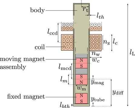
Figure 1. The microgenerator consists of a tube with total length lL, wall thickness lth, bottom thickness lbth and inner radius rt. We wind one or more coils, each of height lc and width wc, around the outside of the tube. We use the same copper wire to wind all the coils, but the direction of the windings alternates for adjacent coils. Each coil consists of nz windings in the vertical direction and nw windings in the horizontal direction. The distance between the centers of adjacent coils is lccd. We fix a magnet to the bottom of the inside of the tube. Above this, we place a levitating magnet assembly, with its bottom-most pole matching the upper pole of the fixed magnet. The magnet assembly consists of one or more identical permanent magnets, each with width wm and height lm. When the assembly consists of multiple magnets, we match adjacent poles and separate adjacent magnets with an iron spacer of width wm such that the spacer separates the centers of the constituent magnets by length lmcd. We use an identical magnet for the fixed magnet at the bottom of the tube. When the levitating assembly consists of a single magnet, spacers are not needed. We use ytube as a reference point to the absolute position of the microgenerator body relative to some fixed stationary point at which analysis begins. Similarly, ymag references the absolute position of the center of the lowermost magnet in the magnet assembly, relative to the same fixed point as ytube.
Download figure:
Standard image High-resolution imageWe attach the microgenerator to a mobile fixture, such as an animal's leg. As the fixture moves, the levitating magnet assembly inside is free to move, thus inducing a changing flux in the coil(s) which, in turn, induces an emf. We can harvest this emf and use it to power electronics.
3. Analytical electromechanical system model
In this section, we first derive an expression for the analytical electromechanical model in terms of its components. We then derive expressions for the behaviour of each component before finally combining the component expressions with the analytical electromechanical model to produce a single set of differential equations that describe the complete analytical electromechanical system.
3.1. Equations of motion
Consider figure 2(a), which shows the free-body diagram and electrical circuit of the microgenerator. The force experienced by the levitating magnet (due to the fixed magnet below it) is Fmag, the frictional force opposing motion is Ffric, the electrical damping force due to the opposing magnetic field (induced by the current flowing through the coil) is Fdamp, and the force the magnet assembly experiences when it collides with the top of the microgenerator body is Ftop. The external force acting on the tube and causing it to accelerate is Facc. We can derive an expression for the mechanical component of the system model in terms of these forces. Unless otherwise indicated, all derivatives will be with respect to time.
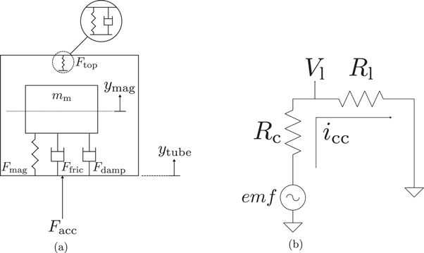
Figure 2. Free-body diagram of the mechanical system (a) and circuit diagram of the corresponding electrical system (b). (a) The mechanical system model consists of a levitating magnet with mass mm whose center is at position ym, suspended inside a tube with position yt. Fmag is the force experienced by the levitating magnet due to the fixed magnet, Ffric is the opposing force experienced due to friction and Fdamp is the force experienced due the opposing magnetic field induced by the current flowing through the coil within the electrical system. Facc is the external driving force that acts on the tube. Ftop is the force the magnet experiences when it collides with the top of the microgenerator body. (b) A variable voltage source and two resistors model the electrical system. The open-circuit voltage produced by the levitating magnet is emf. The closed-circuit current is icc. The internal resistance of the coil is Rc and the load resistance is Rl. Vl is the voltage over the load.
Download figure:
Standard image High-resolution imageWith reference to figure 1, recall that ymag is the position of the center of the moving magnet (with mass mmag) and ytube is the position of the microgenerator tube (with mass mtube). Now let:


then,


Note that ydiff represents the displacement of the center of the lowermost magnet in the assembly, measured relative to the bottom of the tube, as shown in figure 1.
We can further expand equations (3) and (4) by adding an expression for the emf  induced in the coil, which is itself a function of ydiff. Let ϕ be the flux linkage between the magnet assembly and the coil, as a function of the relative magnet position ydiff, then from Faraday's Law:


To describe the analytical electromechanical model, we thus need to find expressions for Fmag, Ffric, Fdamp, Ftop, and ϕ.
3.2. The microgenerator body length, lL
Consider the microgenerator design shown in figure 1, which shows the dimensions of the individual microgenerator components, and figure 3, which shows the position of the magnet assembly at rest and at its maximum height. If the microgenerator body is to allow the magnet assembly to move entirely through all the coils, we must define the height of the microgenerator body lL as:

where lbth is the thickness of the bottom of the tube, lth is the thickness of the tube everywhere else, lhover is the distance between the fixed magnet and the magnet assembly at rest,  is the distance between the magnet assembly and the lowermost coil at rest. It is also the distance between the magnet assembly and the uppermost coil at the magnet assembly's maximum height. Parameters c and m are the number of coils and magnets, respectively, while lccd and lmcd are the distances between the centers of adjacent coils and centers of adjacent magnets, respectively, and parameters lc and lm are the lengths of each individual coil and magnet, respectively.
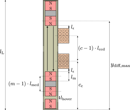
Figure 3. We arrange the coils so that the bottom edge of the lowest coil is a distance  from the upper edge of the magnet assembly at rest. In this situation the magnet assembly hovers at a distance of lhover above the fixed magnet. We achieve this by deliberately positioning the center of the bottom coil cc to satisfy this condition. Furthermore, the magnet assembly body must be sufficiently long so that the magnet assembly can move through all the coils and, at its maximum position, provide a distance
  between the upper edge of the top coil and the lower edge of the magnet assembly. The maximum possible displacement of the magnet assembly is
  .
.
Download figure:
Standard image High-resolution imageFrom equation (7), note the disproportionate effect of m, lmcd, and lm (which are all parameters related to the magnet assembly) on lL: it is spatially expensive to have a large magnet assembly.
3.3. The magnetic spring force, Fmag
Due to the pole-matching, the levitating magnet experiences a repulsive force from the fixed magnet at the bottom of the microgenerator body, forming a magnetic spring. We approximate the force experienced by the levitating magnet due to the magnetic spring by a sum of three decaying exponentials, which can approximate the exponential decay inherent between two magnetic poles:

where si is the size of each exponential and is an element of S = [s1, s2, s3] and ai is the rate of decay of each exponential and is an element of A = [ai , a2, a3]. We find the elements of S and A using a curve-fitting procedure described in section 5.
3.4. The mechanical friction force, Ffric
We approximate the mechanical loss due to friction by modelling it as a constant damper that is proportional to the mass of the magnet assembly:

where bm is the damping coefficient, which must be experimentally determined, and mm is the mass of the magnet assembly.
3.5. The rebounding impact force, Ftop
We model the rebounding impact force experienced by the levitating magnet as it encounters the top of the microgenerator body as a joint spring-damper system that is not physically fixed to the levitating magnet. This can be adequately represented by the following relationship:

where Q is the strength of the spring,  is the maximum magnet assembly displacement, relative to the tube, before it impacts the top cap of the tube. Note that we relate
  to the length of the microgenerator body with the following expression:

Also, in equation (10), bf is the damping constant, which models the energy lost during the impact. We determine the value of bf using a parameter search process, described in section 5. H is the Heaviside step function of the form:

which ensures that Ftop acts on the levitating magnet only when it impacts the top of the microgenerator body. To model a rebounding impact with the top of the microgenerator body that has little 'compression', we select the spring strength Q to have a large value, Q = 1e7. The larger the spring strength, the less compression occurs, approximating a solid material. Note that a large value of Q does not influence the speed with which the magnet assembly rebounds after impact (this is, instead, determined by bf), as the law of conservation of energy is not violated.
3.6. The flux linkage, ϕ
In order to calculate the electrical damping force Fdamp and the emf, we need to model the magnetic flux linkage ϕ passing through the coil. The magnetic flux linkage is the amount of magnetic flux, produced by the magnetic field of the magnet assembly, that passes through the windings of the coil. We model the flux linkage as a function of the relative displacement between the magnet assembly and tube ydiff, the number of windings in the axial direction nz, the number of windings in the radial direction nw and our particular choice of magnet. We assume a single choice of magnet throughout our described process.
To develop our expression for the flux linkage, we begin by modelling it for a single-coil, single-magnet configuration. We then systematically extend this to a generalized model that we can apply to any number of coils and number of magnets.
3.6.1. Single-coil, single-magnet configuration
The simplest configuration of our microgenerator has one coil and one magnet. We have not been able to determine a closed form expression for the true value of ϕ as a function of coil parameters nz and nw, and believe this is not possible because the relationship is dependent on a number of hidden parameters, such as the magnetic field strength vector and magnetization of the magnet assembly, as well as the field's interaction with each winding in the coil. Hence, we will model the flux linkage as a weighted sum of k smooth kernels, with the kernel centers evenly distributed about ![${y}_{\mathrm{diff}}\in [0,{y}_{\mathrm{diff},\ \max }]$](https://content.cld.iop.org/journals/2399-6528/6/5/055018/revision2/jpcoac77d6ieqn8.gif) , and sampled over evenly distributed points p ∈ ydiff. Modelling the flux linkage in this way provides two advantages. Firstly, such superpositions of smooth kernels have the ability to approximate a wide variety of smooth functions. Secondly, and more importantly, if we can find the relationship between nz and nw and the kernel approximation (for a particular choice of magnet), we can then predict the flux linkage as a function of nz and nw. We explore this particular concept further in section 6, where we construct a model that can predict the flux linkage from nz and nw for our particular choice of magnet.
, and sampled over evenly distributed points p ∈ ydiff. Modelling the flux linkage in this way provides two advantages. Firstly, such superpositions of smooth kernels have the ability to approximate a wide variety of smooth functions. Secondly, and more importantly, if we can find the relationship between nz and nw and the kernel approximation (for a particular choice of magnet), we can then predict the flux linkage as a function of nz and nw. We explore this particular concept further in section 6, where we construct a model that can predict the flux linkage from nz and nw for our particular choice of magnet.
Let us define each kernel as a function similar to that of a Gaussian radial basis function. If we define the center of a kernel as kc and recall that we sample each kernel over evenly spaced points p, then we can express an individual kernel as:

In equation (13) kc controls the kernel location (which is set differently for each kernel so as to evenly distribute the kernels over ![${y}_{\mathrm{diff}}\in [0,{y}_{\mathrm{diff},\ \max }]$](https://content.cld.iop.org/journals/2399-6528/6/5/055018/revision2/jpcoac77d6ieqn9.gif) ), D controls the kernel magnitude and s controls the kernel width. We treat D and s as constants that we select, and thus omit D and s as parameters.
), D controls the kernel magnitude and s controls the kernel width. We treat D and s as constants that we select, and thus omit D and s as parameters.
Next we combine the kernels into matrix K with dimensions (k, np ), where k is the number of kernels and np is the number of linearly spaced points in p. If we take the dot product of K with weight vector wk , we can approximate the flux curve with the resulting vector Φ:

where we assume that our choice of wk produces a weighted sum that approximates a smooth curve with a single peak at pc, which corresponds to the center of the flux curve. We can easily achieve the desired pc by linearly shifting the discrete sampling points p and kernel centers kc of the kernels present in matrix K.
Thus, by carefully manipulating wk , we can approximate different flux curve shapes. We show an example of this with pc = 5 in figure 4.

Figure 4. We can model a flux curve by taking a weighted sum of k evenly-distributed kernels across a np discrete points. In equation (14), K is the matrix of unweighted kernels (a), (b) shows the kernels as weighted by vector wk and ϕ (pc) is the resulting weighted sum, centered about pc = 5 (c). Manipulating wk allows us to produce different flux curves. (a) Unweighted kernels in matrix K. (b) Kernels weighted by vector wk . (c) Resulting weighted sum vector ϕ (pc = 5).
Download figure:
Standard image High-resolution imageAdditionally, when the levitating magnet's center aligns with the center of the coil, the total flux linkage reaches a peak, since at this position the flux entering and exiting the coil is equal, resulting in a net flux of zero. We can place the peak of ϕ by setting pc equal to the location of the coil's center ϕ (pc = cc) for the single-coil, single-magnet (c = 1, m = 1) case. This allows us to model the position of the coil, relative to the position of the moving magnet.
We deliberately model the flux linkage as a function of the relative displacement ydiff between the magnet assembly and the tube, as this allows us to calculate the induced emf, it's derivative (velocity) and the flux linkage between the magnet and the coil given equation (6). Later, this is further utilized to couple the mechanical and electrical systems.
Note that equation (14) produces a vector of points, while we require a continuous function to later solve the set of equations that describe the electromechanical system. We therefore use a linear interpolation function, Γ, that accepts the resulting weight kernel sum ϕ and a single point p ∈ ydiff as arguments, and returns the interpolated flux value at this point p to define a new function ϕ0:

Now, given a kernel weight vector wk , and a flux curve center pc, we can use equation (15) to estimate the instantaneous flux linkage given the relative position ydiff between the magnet assembly and the coil for the case of c = 1 and m = 1.
3.6.2. Multiple-coil, single-magnet configuration
We now extend the flux model to allow for multiple-coils, but still assume a single magnet in the assembly.
As shown in figure 1, we wind adjacent coils in opposite directions and have their centers offset by the distance lccd. This ensures that, as the magnet assembly moves through the coils, the total flux linkage between the magnet and all coils adds constructively, resulting in an increased induced emf.
Using equation (14) and the knowledge that we space the coils uniformly, we can define an expression for the total flux linkage ϕc≥1,m=1 for the multi-coil, single-magnet configuration by adding the flux linkage contributions due to the individual coils for the spacing between the coil centers lccd:

where cc references the position of the center of the lowermost coil, and c is the number of coils in the configuration.
We cannot make the choice of coil center distance lccd arbitrarily. Consider figure 5, which shows the individual flux linkage due to each coil in a microgenerator with two coils and one magnet (c = 2, m = 1). Note how the flux linkage adds constructively when the gradient of the flux linkage for both coils has the same sign or zero for one of them (regions shown in blue). In contrast, destructive superposition occurs when the gradient of the flux linkage in the coils have opposite signs (regions shown in red). As our goal is to maximize the emf  , we must maximize the constructive superposition and minimize the destructive superposition by selecting an appropriate value of lccd. Figure 6 shows the RMS of the induced emf as a function of lccd for the same microgenerator configuration shown in figure 5, which we calculate by computing the RMS of the derivative of equation (16) (i.e. the emf) with respect to ydiff. We see that, when lccd is too small, RMS is reduced due to destructive superposition. Of particular interest is that an optimal lccd value exists that results in a maximum RMS. We therefore select this optimal value
  to maximize the RMS of the emf:

where  is the emf induced across all coils for the multiple-coil, single magnet microgenerator configuration:

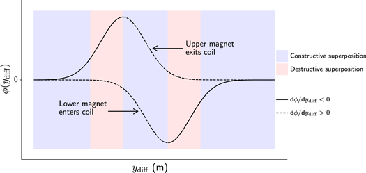
Figure 5. We can illustrate the source of constructive and destructive superposition by considering the individual magnet-coil flux linkage using the example of a two-coil, single-magnet (c = 2, m = 1) microgenerator configuration. The two curves show the respective flux contributions of the two coils as a function of ydiff, as defined in figure 1 and equation (1). Constructive superposition occurs when the coils experience a rate of change of flux in the same direction, or one of them is zero (regions shown in blue). Destructive superposition occurs when the coils experience a rate of change of flux in the opposite direction (regions shown in red).
Download figure:
Standard image High-resolution image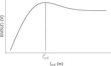
Figure 6. There exists an optimal value for the distance separating the two coil centers  that maximizes the RMS of the emf
  of the two-coil single magnet microgenerator. Any microgenerator where c > 1 should thus use this optimal value of lccd. When the value of lccd is too small, it diminishes the resulting RMS due to destructive superposition of the flux linkage. Increasing lccd, we find the optimal point
  where we maximize the constructive superposition. If we further increase lccd, no superposition of the flux linkage occurs, causing the RMS to approach a stable value that is lower than that of the maximum RMS.
Download figure:
Standard image High-resolution image3.6.3. Single-coil, multi-magnet configuration
Next, we extend our flux model to allow the microgenerator to have multi-magnets, but a single coil. This is similar to the multi-coil, single-magnet configuration described in the previous section.
As shown in figure 1, adjacent magnets in the magnet assembly have opposite polarity, and we separate their centers by a distance lmcd. As for the single-magnet multi-coil microgenerator configuration, this ensures that the flux linkage of each magnet with the coil superimposes constructively, resulting in a larger induced emf. Recall from figure 1 and equation (1) that ydiff is the displacement of the center of the lowermost magnet in the assembly above the bottom of the tube.
We define an expression for the flux linkage between all m magnets and the single coil ϕc=1,m≥1 by adding the terms representing the contribution due to each magnet:

where cc is the location of the center of the coil, and the spacing between the magnet centers is lmcd. Note here that we subtract the flux curve offset for additional magnets from the location of the coil, since ydiff describes the position of the lowermost magnet. This is in contrast to equation (16).
As with the multi-coil, single-magnet configuration, it is again important to select an optimal distance lmcd between the magnet centers, so as to maximize the constructive superposition and minimize the destructive superposition of the flux linkages due to the individual contributions by the magnets. As for the case of multiple coils and a single magnet, selecting a value for lmcd that is too small results in a reduced power output, due to the destructive superposition of the flux linkage. In this particular case, there is also a lower-bound on lmcd due to the practical difficulty of assembling magnets in a pole-matched configuration. We denote this lower-bound as  .
.
By inspecting equations (16) and (19) we see that there is no difference, from the perspective of the resulting flux curve, between the configurations (c ≥ 1, m = 1) and (c = 1, m ≥ 1). Therefore, as in equation (17), there must again exist an optimal value of  that maximizes the RMS of the emf induced for the single-coil, multi-magnet case:

where  is the emf induced across the coil for the single coil, multi-magnet case:

3.6.4. Multi-coil, multi-magnet configuration
Finally, we derive the flux model for the general case in which the microgenerator has multiple coils as well as multiple magnets.
As discussed in section 3.6.3, when a magnet assembly with multiple magnets moves through a single coil, it produces a flux curve described by the superposition of m curves as modelled by equation (19). When there are both multiple coils and multiple magnets, the produced flux curve will be a superposition of c curves, as described by equation (16), where each of these c curves is itself a superposition of m curves, as described by equation (19). Therefore, in this general case, we derive the microgenerator's flux curve from following double summation:

From equation (22) we see that both the coil-center distance lccd and the magnet-center distance lmcd affect the flux curves in the same way. Therefore, their optimal values must be equal:

As an example of a multi-coil, multi-magnet flux curve, we show ϕc=2,m=2(ydiff), the case of two coils (c = 2) and two magnets (m = 2), in figure 7, together with the four individual flux curves superimposed by equation (22). Note the alternating polarity of each individual flux curve, due to the alternating polarity of adjacent magnets and the alternating direction in which we wind adjacent coils. In this particular example, the optimal coil center  , and magnet center
  distance are used.
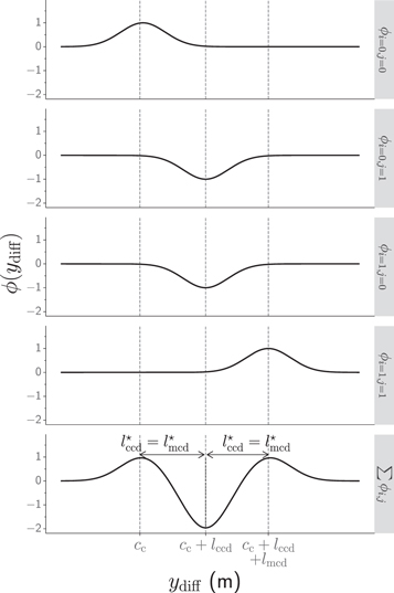
Figure 7. Here we show a particular case with c = 2 coils and m = 2 magnets as an example. We sum the four individual flux linkages (first four plots), each given by equation (14), as described by equation (22) to produce the final flux curve profile of the microgenerator (bottom plot).
Download figure:
Standard image High-resolution imageNote that, the values of lccd and lmcd are independent of the number of coils c and number of magnets m. As a result, we only need to find either  or
or  for one of two cases: (c = 2, m = 1) or (c = 1, m = 2), respectively. We can then infer the other distance parameter using equation (23).
3.7. Coil center distance, cc
From figure 3, we can see that it is possible to calculate the coil center distance, cc, from the magnet length lm, the magnet center distance lmcd (in the case of multiple magnets), the magnet assembly hover height at rest lhover, and the chosen distance l between the top edge of the magnet assembly and the lower edge of the first coil. This ensures that the magnet assembly has little coupling with the coil(s) at rest, thus increasing the possibility of realizing a large rate of change of flux, and thus emf, when the microgenerator experiences motion. From figure 1 and 3, we can express the coil center distance cc as follows:

We can calculate the value of lhover using the magnetic spring force from equation (8) and the weight of the magnet assembly:

3.8. Coil resistance, Rc
We must know the coil resistance Rc in order to calculate the electrical damping force, Fdamp, and therefore we must define a model for it. We first model the length of the copper wire used in the coil, lcoil. Given the assumed square-packing configuration of the windings and the parameters shown in figure 8, we can express the length of the wire as:


where nw is the number of windings in the radial direction, nz is the number of windings in the axial direction, lth is the tube wall thickness, rt is the inner radius of the microgenerator tube, and rc is the radius of the copper wire used for the winding.
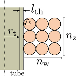
Figure 8. A detai/t view of a cross section of the microgenerator body and a wound coil. The microgenerator tube has an inner radius of rt and a wall thickness of lth. The wire used for the winding has a radius of rc. The coil consists of nz windings in the vertical direction and nw windings in the radial direction.
Download figure:
Standard image High-resolution imageOnce we have found lcoil, we can calculate the total resistance of the coil:

where β is the wire gauge's resistance per unit length, which has a unit of Ω/mm.
3.9. The electrical damping force, Fdamp
As a magnet moves through a coil, it induces an emf. If there is a closed circuit, as shown in figure 2(b), Lenz's Law states that a current will flow in the direction that induces a magnetic field which opposes the magnetic field inducing the current (in this case the magnet assembly). This opposing magnetic field exerts a force on the magnet assembly that is proportional in magnitude to the current flowing through the coil. We therefore model the electrical damping force as directly proportional, with constant be, to the current icc flowing through the coil:

Given the electrical circuit in figure 2(b), we can calculate the closed-circuit current icc as:

Substituting equations (6) and (31) into (30) gives the final expression for the electrical damping force:

3.10. The complete system of equations
By substituting equations (8) to (32), (22) and (10) into (3), (4) and (6), we obtain a set of equations that models the joint mechanical and electrical system:


Using equations (33) to (35), we can numerically solve for yt, ym, and ϕ as functions of time, given initial conditions and input acceleration force Facc. We can then use the solutions for yt, ym and ϕ to calculate the complete predicted electrical and mechanical behaviour of the microgenerator.
There are three categories of parameters that we require in order to solve equations (33) to (35): a set of parameters that are chosen by inspection, a set of parameters that are optimized to minimize the difference between model predictions and empirically-measured (or simulated) data, and a set of variable parameters that we can optimize to maximize the power that is generated.
The first category consists of parameters that we choose, by inspection, at the outset to conform to practical constraints. These include the specific magnet type and shape (controlled by lm and wm) used in the magnet assembly and magnetic spring, the inner radius rt of the tube, the tube wall thickness lth, coil wire radius rc (and thus also the coil resistance per unit length β), the load resistance Rl, the magnet assembly to coil distance l
and the microgenerator tube length lL. We discuss the parameters belonging to this category in greater detail in section 4.
The second category of parameters consists of those that describe inherent physical properties of the microgenerator behaviour. These parameters are optimized to minimize the difference between the system model predictions and empirical measurements using an evolutionary process in conjunction with a number of physical reference devices. These include the magnet spring parameters (S, A), the mechanical friction coefficients bm, the electrical damping constant be, and the impact force damping constant bf. The process of discovering these parameters is discussed in section 5.
The third category of parameters consists of those that can be varied to alter the behaviour of the microgenerator, but without affecting the predictive accuracy of the model. We optimize these parameters to discover microgenerator designs that maximize the power delivered to the load. These include the number of coils c, number of magnets m, coil-center distance lccd, and magnet-center distance lmcd. The base flux waveform ϕ0 is a special case that also falls into this category, because it is dependent on the number of coil windings in the axial direction nz and radial direction nw (in addition to the choice of magnet), both of which we optimize to maximize load power. As a result, we give special attention to how we obtain ϕ0 from nz and nw in section 6. Although not strictly an optimization parameter, we include the center height of the lowermost coil cc in this parameter category also, since the coil center height cc depends on parameters m and lmcd (equation (24)) and we therefore need to update its value each time we change m and lmcd during the optimization process. We discuss the optimization process for this third category of parameters in section 7.
The benefit of equations (33) to (35) is that, once we determine the first two categories of parameters (chosen parameters, and discovered parameters), we can predict the behaviour of the microgenerator for any input excitation Facc and for any set of parameters that fall into the optimization category. This allows us to optimize the design of the microgenerator for any specific excitation.
It is critical to note that the parameters of the second and third categories (found parameters and optimized parameters) will be specific to the first category of parameters (those that we chose). As a result, if we modify any of the hand-chosen design parameters, we must repeat both the parameter discovery (including acquiring new measurement data) and parameter optimization processes for valid results. This is a direct result of the wide range of inter-dependencies between the parameters that are inherent to this microgenerator architecture, and contributes considerably to the difficulty of optimization.
4. Parameter selection
The microgenerator design includes a number of parameters that do not describe inherent behaviour in the electromechanical system and that are therefore not part of the parameter discovery or optimization processes, and are chosen arbitrarily. We provide these chosen parameters and their values in table 1, and we consider them as constant values for the remainder of this paper.
Table 1. The parameters that we must choose before proceding with parameter discovery or parameter optimization. We treat these values as constants for the duration of this work, and results based on this parameter selection are entirely specific to these particular values. Refer to figures 1 and 3 for the definition of the dimensions.
| Description | Parameter | Value |
|---|---|---|
| Coil wire radius (mm) | rc | 0.0715 |
| Coil resistance per unit length (Ω/mm) | β | 1079 × 10−6 |
| Magnet length (mm) | lm | 10 |
| Magnet diameter (mm) | wm | 10 |
| Magnet assembly to coil distance (mm) |
l
| 5 |
| Tube inner radius (mm) | rt | 5.5 |
| Tube bottom thickness (mm) | lbth | 3 |
| Tube wall thickness (mm) | lth | 1 |
| Load resistance (Ω) | Rl | 30 |
We choose identical N38-grade neodymium magnets for the magnet assembly and the fixed magnet at the bottom of the tube. The magnets are cylindrical with a length lm = 10 mm and diameter wm = 10 mm. We therefore select the inner radius of the tube to be rt = 5.5 mm, to provide sufficient clearance for the magnet assembly to move freely. We selected the tube wall thickness to be lth = 1 mm, as this was the minimum that we could achieve using an additive 3D printing process with PLA as the printing material. We select the bottom of the tube to be lbth = 3 mm thick. We selected American Wire Gauage (AWG) 35 copper wire to use for the coils, which has a radius of rc = 0.0715 mm and a resistance per unit length of β = 1079 × 10−6Ω/mm. We select the distance between the uppermost magnet edge and the lower edge of the bottom coil to be l
= 5 mm. Finally, we select our target load to be a constant resistive load of 30Ω.
Note again that all subsequent calculations, such as the parameter discovery in section 5 and parameter optimization in section 7 are entirely specific to this particular choice of parameter values. If the value change, we must repeat all subsequent calculations to achieve correct results.
5. Parameter discovery
Having chosen and fixed some parameters in section 4, we now turn to describing a process to find those parameter values in equations (33) to (35) that must be determined by measurement or simulation. These are the magnetic levitation force Fmag parameters S = [s1, s2, s3], A = [a1, a2, a3], the magnet assembly levitation height lhover, which we require to determine the coil center height cc, the mechanical damping coefficient bm that models the mechanical losses due to friction, the constant be that models the coupling between the electrical damping force Fdamp and the coil current, and the damping coefficient bf required to model the impact force Ftop.
We show an overview of the parameter discovery process in figure 9. First, as an independent step, we determine the magnetic levitation force parameters S and A using least squares regression and FEA data. Then, we physically construct a number of reference microgenerator devices, with the same values selected in section 4, and measure each reference devices' behaviour and output experimentally, including the acceleration of the microgenerator tube  . We then use an evolutionary algorithm to find the remaining unknown parameters bm, be and bf. The algorithm iteratively samples new possible values for bm, be and bf based on previous sampled values, which we substitute into our model equations (33) to (35) together with the magnetic levitation force parameters S and A. We then solve these parameterized model equations using the measured microgenerator tube accelerations
  as the input excitation. Next we update the best parameter values if they produce a lower loss than the current best. We repeat this process for a large number of iterations, resulting in set of parameters that best predict the measured behaviour of the reference microgenerator devices.
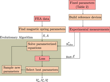
Figure 9. An overview of the process that we use to find parameters that describe inherent physical properties of the microgenerator. Note again that this process is specific to the the second category of parameters, i.e. the parameters that are optimized to minimize the difference between the system model predictions and experimentally-measured or simulated data. First, we use FEA data to find the magnetic spring parameters S and A. In our particular case, we construct four references devices, and take ground truth measurements for the relative magnet assembly position ydiff, the induced emf  and the acceleration applied to the microgenerator tube
  . We then solve the set of parameterized equations (33) to (35) for new, sampled values of the mechanical damping coefficient bm, the electromechanical damping coupling factor be and the impact force damping coefficient bf, using an evolutionary algorithm. We use the measured tube acceleration from experimental measurements as the input excitation. After solving the parameterized model equations, we compute the loss between the behaviour predicted by the simulation and the measure behaviour, and update our set of best parameters with the newly-suggested parameters if they result in a lower loss. After a large number of such iterations, we are left with the an optimized parameter set
  .
.
Download figure:
Standard image High-resolution imageNote that, while solving the system equations during the parameter search process, we replace the base flux linkage curve ϕ0 with flux linkage curves obtained using FEA. This prevents potential inaccuracies in the base flux linkage curve model, as given in equation (15), from propagating through the system, resulting in an inaccurate selection of parameter values.
5.1. Magnetic levitation force parameters S and A
We find the magnetic levitation force parameters of S = [s1, s2, s3] and A = [a1, a2, a3] by fitting equation (8) to data acquired by FEA simulation for the specific magnet shape and type that we selected in section 4.
We use the software package FEMM [36] to carry out the FEA force simulation. The axisymmetric test setup shown in figure 10. The simulation consists of an axially-magnetized magnet with a diameter of 10 mm and a height of 10 mm placed at a reference position. We specify the magnet material as N38 grade neodymium. The magnet dimensions and material match those of the magnets chosen for the physical microgenerator device. We position an identical magnet directly above the reference magnet, but rotated so that its bottom pole matches the top pole of the reference magnet. We translate top magnet upwards in 1 mm increments (starting at a distance of 0 mm and ending at 60mm) from the reference magnet, and calculate force experienced by the top magnet as a function of the distance between the two magnets.
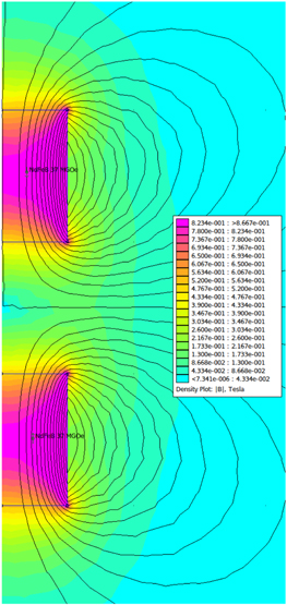
Figure 10. The axisymmetric FEMM simulation setup which consists of two identical N38 grade neodymium magnets. We translate the top magnet's position upwards in 1 mm increments (starting at a distance of 0 mm and ending at 60mm) in order to calculate the force experienced by the top magnet as a function of the distance between the two magnets.
Download figure:
Standard image High-resolution imageUsing this FEA force data, we find the parameters S and A using a least squares optimization [37, 38]. For the particular magnet under consideration, we found that the parameter values that produce the best fit are S* = [5.134, 26.291, 0.1256 × 10⁶], and A* = [0.122, 0.352, 11.609]. A comparison between the FEA simulation and the curve-fit model of the magnetic levitation force in figure 11 shows strong agreement between the proposed model and the results of the FEA simulation.
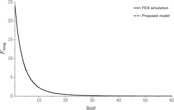
Figure 11. Comparison of the force experienced by the levitating magnet as predicted by FEA simulation and the proposed magnet spring model, given by equation (8). We observe strong agreement between the FEA simulation and the proposed magnetic spring model.
Download figure:
Standard image High-resolution image5.2. Parameters bm, be and bf
Next, we describe the parameter search process used to find values for the mechanical damper coefficient bm, the electromechanical damper coupling factor be and the damping coefficient bf of the impact force Ftop. This process requires empirical, measured ground truth data of the relative magnet assembly position ydiff, the induced emf  and the corresponding driving acceleration
  , as well as our results for the magnetic spring parameters S and A, discussed in section 5.1.
5.2.1. Reference devices and ground truth data collection
We require ground truth data in order to find parameters bm, be and bf. To achieve this, we physically construct and assemble ndevices = 4 possible reference microgenerator devices (A, B, C and D), each with different sets of chosen parameters as shown in table 2. It is important to have sufficiently many reference devices with differing designs to sufficiently explore and generalize over a wide design space. As a result, we configured the reference devices with substantial differences in their design parameters. For example, each device's coil has a different number of windings N, coil length lc, coil width wc, coil center cc and coil resistance Rc. All other parameters match those chosen in section 4 and given in table 1.
Table 2. Microgenerator parameters for the four reference devices used to obtain ground truth data for the parameter search process.
| Description | Param. | A | B | C | D |
|---|---|---|---|---|---|
| Number of coils | c | 1 | 1 | 1 | 1 |
| Number of magnets | m | 1 | 1 | 1 | 2 |
| Coil wire radius (mm) | rc | 0.0715 | 0.0715 | 0.0715 | 0.0715 |
| Coil center position (mm) | cc | 72 | 74 | 76 | 90 |
| Coil length (mm) | lc | 8 | 12 | 14 | 25 |
| Coil thickness (mm) | wc | 0.75 | 0.67 | 0.48 | 1.43 |
| Total coil windings | N | 295 | 395 | 330 | 1760 |
| Coil resistance (Ω) | Rc | 12.5 | 23.5 | 17.8 | 80.1 |
| Magnet length (mm) | lm | 10 | 10 | 10 | 10 |
| Magnet diameter (mm) | wm | 10 | 10 | 10 | 10 |
| Magnet center distance (mm) | lmcd | — | — | — | 24 |
| Tube inner radius (mm) | rt | 5.5 | 5.5 | 5.5 | 5.5 |
| Tube bottom thickness (mm) | lbth | 3 | 3 | 3 | 3 |
| Tube wall thickness (mm) | lth | 1 | 1 | 1 | 1 |
| Load resistance (Ω) | Rl | 30 | 30 | 30 | 30 |
| Microgen. body length (mm) | lL | 120 | 120 | 120 | 150 |
Table 3. Parameters that are treated as optimizable. Each of these parameters are optimized using the search process presented in figure 20, in order to maximize the mean power  delivered to the load.
| Parameter | Description |
|---|---|
| c | Number of coils |
| m | Number of magnets in the magnet assembly |
| nz | Number of coil windings in the axial direction per coil |
| nw | Number of coil windings in the radial direction per coil |
| lmcd | Distance between the centers of each subsequent magnet |
| lccd | Distance between the centers of each subsequent coil |
We 3D-printed the reference device bodies using PLA through an additive process, and wound the coils using a speed-controlled lathe.
We indicate the experimental setup in figure 12. We mounted a reference microgenerator to one end of a base plate and a camera, capable of high-framerate video, to the opposite end. We also mounted an accelerometer (ADXL345) to the base plate, directly behind the microgenerator. We connected the microgenerator coil to a Schottky diode full-wave bridge rectifier, whose rectified output powers a static resistive electrical load. This load voltage was attenuated using a voltage divider, and connected to the ADC input of a microcontroller (Teensy 3.5). We measured the voltage attenuation factor to be approximately 2.92: 1. Furthermore, each reference microgenerator body was manufactured with an axial groove down the sides, thereby exposing the magnet assembly to the camera. We programmed the microcontroller to record both the accelerometer output and the scaled load voltage, while the camera recorded video footage of the magnet assembly moving through the microgenerator body. This experimental setup allowed us to record both the mechanical system behaviour and the electrical system behaviour of the reference microgenerators simultaneously.
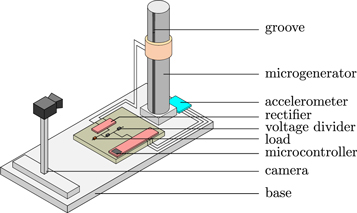
Figure 12. The experimental setup used to take ground truth measurements. We attached the microgenerator to one end of the base plate and a camera that can record high framerate video to the other end. An accelerometer was attached to the base plate directly behind the microgenerator. We rectified the output of the microgenerator coil using a Schottky full wave bridge rectifier, which we attached to a static resistive load. We measured the load voltage using the ADC input of the microcontroller, via a resistive voltage divier.
Download figure:
Standard image High-resolution imageTo generate a ground truth sample, the camera and microcontroller recorded simultaneously at 120 FPS and 1600 Hz respectively. The base plate was moved in an approximately footstep-like motion for a single cycle. As illustrated in figure 13, the motion consists of an upwards acceleration across a distance of approximately 15 cm, a brief pause, and a subsequent downward acceleration followed by an impact. Figure 13(b) shows a typical such accelerometer measurement in the y-direction. We repeated this process ninput = 7 times for each device.
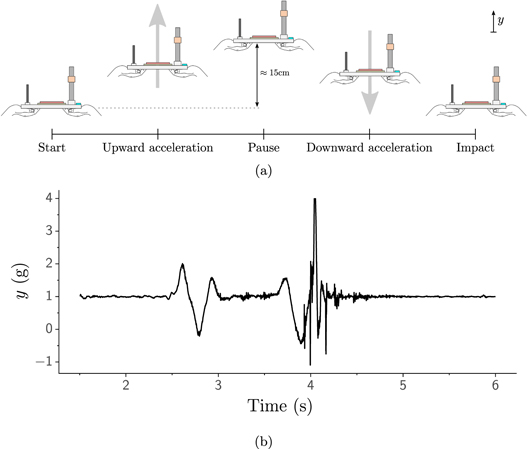
Figure 13. (a) A single cycle of the footstep-like input excitation which apply to the experimental setup shown in figure 12. The motion consisted of an upward acceleration from rest, a brief pause, and a downward acceleration terminating in an impact. The difference between the maximum and minimum vertical positions of the base plate is approximately 15 cm. (b) An example of the signal measured by the accelerometer in the y (vertical) direction as a result of the motional illustrated in figure 13(a), after smoothing. In this case, the impact occurred at 4.0 s.
Download figure:
Standard image High-resolution imageAfter data collection, we labeled the position of the magnet assembly for each frame in the video recording. We also descale the ADC voltage measurements, using the voltage divider ratio, to calculate the true total load voltage. We use an Savitzky-Golay filter, which is a type of filter that is both simple to implement and easy to tune [39], which was empirically-tuned to reduce noise that was present on the output of the accelerometer.
5.2.2. Search process
The parameter search procedure is shown in figure 14. This process combines the ground truth measurements and our system of model equations to iteratively find the best set of parameter values for bm, be and bf.
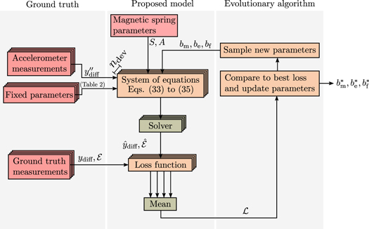
Figure 14. Detailed illustration of the search process used to find parameter values bm, be and bf. The process includes an evolutionary algorithm, which samples new candidate values of bm, be and bf. We substitute these candidate values, in conjunction with the magnetic spring parameters S and A and fixed device parameters from table 1, into the system of model equations equations (33) to (35) for each reference device, of which there are ndev = 4. Using the measured ground truth accelerometer measurements (nacc = 7 per device) as input excitation, we solve each instantiated system of model equations using a numerical solver. The results are then compared to the corresponding ground truth measurements and we calculate the mean loss using equation (36). We compare this loss to the current best, and, if a set of candidate parameters results in a lower loss, we update the current best set of parameters  and
and  .
.
Download figure:
Standard image High-resolution imageThe search process begins by sampling new values for parameters bm, be and bf provided by the (1+1) evolutionary algorithm [40], as implemented in the Nevergrad computational library [41]. We deliberately chose to use an evolutionary algorithm to avoid the combinatorial explosion that occurs when using a exhaustive gridsearch with fine-grained parameter values. The sampled parameter values, along with magnetic spring parameters S and A and fixed parameters from table 1, are then substituted into the system of model equations (33) to (35), for each device. Next, we solve the model equations for each device using each of the nacc = 7 corresponding measured acceleration as the input excitation using an ODE numerical solver of type Explicit Runge-Kutta method of order 5(4) [42], implemented in the SciPy library [38]. The solution provides estimates for the relative magnet position  and the load voltage
  , the latter of which is then used to calculate a loss relative to the corresponding ground truth measurement of the load voltage Vl. We define our loss as the mean normalized load power difference across each reference device and every corresponding input excitation:

where  is the mean normalized load power difference for the ith reference device:

Here,  is the mean power dissipated in the load for the jth input excitation for the ith reference device, and
  is the corresponding ground truth measurement. The mean load power is calculated as follows:

After calculation, we return the loss to the evolutionary algorithm, which updates the current best parameter set  and
and  if we find the loss is better than the current best. We repeated this process for nevo = 2000 iterations, in an effort to converge to a parameter set that minimizes the loss function.
5.3. Search results
The search process found a parameter set of  and
and  that minimized the loss function.
To evaluate these parameter values, we again executed the procedure shown in figure 14, this time using  and
and  , and record the predicted relative magnet displacement
  and predicted load voltage
  . We then evaluate our model according to a number of criteria.
To evaluate temporal accuracy, we calculate the dynamic time warping (DTW) distance between the measured and the computed relative magnet distances and load voltages. This gives an indication of how well we are able to model the mechanical component and electrical component, respectively, of our reference microgenerators.
The DTW algorithm computes the degree to which two temporal signals can be made to align in time [43, 44], if we allow a certain degree of stretching and compression of the time axes. As a result, the smaller the DTW distance, the more similar two signals are in terms of their time behaviour. The literature reports DTW as a more robust measure of similarity than Euclidean (and related) distance metrics in multiple applications [45].
In addition to the DTW, we also calculate the normalized RMS difference between the measured and computed load voltages. This measure indicates how accurately the system model predicts the eventual overall power delivered to the load.
To ensure comparable results, we constrain the computed and the measured signals to the same length, and use interpolation to achieve the same fixed sampling rate for both. For DTW, we normalize the calculated distance by dividing it by the number of samples in the ground truth signals. This allows for ground truth measurements of different lengths to be compared. The normalized DTW distance between the computed and measured relative magnet distances is  and the normalized DTW distance between the computed and measured load voltages is
  . The normalized RMS-difference of the computed and measured load voltage is
  . The RMS-difference is normalized by dividing by the RMS of the measured signal:

Figure 15 shows  ,
,  and
and  as a function of the evolutionary loss function
  , defined in equation (36). Each point represents one of the possible parameter sets of bm, be and bf sampled by the evolutionary algorithm during for each of the nevo = 2000 iterations during the parameter search process. The final chosen parameter set (consisting of
  and
and  ) that minimizes
  is indicated in a different color and with arrows. We observe that every measure generally decreases as the loss decreases. This is significant, as it indicates that our parameter search process minimizes the loss (which is the difference between the calculated and measured load power as per equation (36)) by finding values of bm, be and bf that result in accurate predictions of the time-domain mechanical and electrical behaviour of the microgenerator devices. For example, it would be entirely possible for the parameter search process to find parameters that give accurate power predictions, but inaccurate time-domain behaviour predictions. Figure 15 indicates that this is not the case: our proposed search process (in conjunction with our proposed model) finds parameter values that lead to accurate time-domain behaviour prediction, which in-turn results in accurate load power estimations.
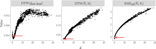
Figure 15. The normalized DTW distance between the predicted and measured relative magnet assembly displacement  , the normalized DTW distance between the predicted and measured load voltage
  and the normalized RMS difference between the predicted and measured load voltage
  , with the calculated evolutionary loss
  , given by equation (36), on the x-axis. Each point represents one of the nevo = 2000 points sampled by the evolutionary algorithm during the parameter search. The final parameter set (i.e.
  and
and  ) that minimizes the loss
  is indicated. We observe that every measure generally improves as the computed evolutionary loss decreases.
Download figure:
Standard image High-resolution imageOf interest is that the minimum value of  does not perfectly coincide with the minimum loss
  . This indicates that, of all the possible parameter sets that were sampled, some lead to more accurate estimation of the mechanical time-domain behaviour, but worse estimation of the load power. This indicates the possible existence of some inaccuracies of the proposed model (possibly due to simplifying assumptions) or in the ground truth data collection process (possibly due to noise), or both. Notably, however, the difference between the parameter sets that lead to the best value of
  and the best value of
  is small, such that it does not significantly affect our ability to estimate ydiff.
We inspect the results for the best parameter set in  and
and  in figure 16, which shows distributions of the normalized Dynamic Time Warping (DTW) distance between the computed and measured values of the relative magnet assembly displacement
  , the normalized DTW distance between the predicted and measured load voltage values
  and the normalized RMS-difference of the computed and measured load voltage
  for each reference device. We see generally good agreement between the predicted and measured results, indicating that the parameters of
  and
and  found in the previous section are both accurate and able to generalize to varied microgenerator designs. In particular, note that the predicted load voltage RMS is almost always within 25% of the measured result. This is noteworthy given the free-form nature of the experimental setup, and suggests that we can be reasonably confident in the model's ability to accurately predict the behaviour and load power of the energy harvester with parameters
  and
and  .
.
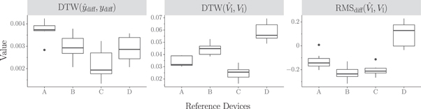
Figure 16. A box-plot distribution estimation, showing the median (horizontal line), minimum (lower whisker), maximum (upper whisker), interquartile range (upper and lower hinges) and outliers (points) for the normalized DTW distance between the predicted and measured relative magnet assembly displacement  , the normalized DTW distance between the predicted and measured load voltage
  and the normalized RMS difference between the predicted and measured load voltage
  .
.
Download figure:
Standard image High-resolution image6. Mapping from coil features to flux curves
We now turn to the last component we require before our final power optimization process can take place: we must model the mapping from the coil features to the flux curve defined in equation (14).
6.1. Flux curve model
The relationship between coil parameters (nz and nw), magnet properties and the resulting base flux curve ϕ0 is not easily determined. The calculation is typically performed using finite element analysis (FEA), which is computationally expensive and therefore not suitable to an iterative application. We propose an alternative method, which only uses FEA initially to generate a training dataset. This dataset is subsequently used to train a linear model for the computation of ϕ0 that is inexpensive to apply for arbitrary values of nz and nw, including those not in the training set.
Recall the model given by equation (14), which approximates the flux curve ϕ by a weighted sum of k kernels across np points, defined as matrix K, by multiplying with a weight vector wk . Since we fix K, we can consider the elements of weight vector wk as trainable parameters.
If we attempt to make a prediction of the weight vector  as follows:

we can define a linear model that does so given some coil features x:

This allows us to modify the model in equation (14) to predict the flux curve directly from the coil features:

where x is an f-dimensional row vector, where f is the number of features, and Ww is a matrix of feature weights with dimensions (f, k).
We can extend this to the general case for n sets of coil features X = [x1, x2,...,xn
] to produce a corresponding set of n flux curve predictions  :
:

where K still has dimensions (np, k), X has dimensions (n, f), and Ww
still has dimensions (f, k). The resulting output  has dimensions (n, np). We treat the number of kernels k, the shape parameter s and the kernel magnitude D as model hyperparameters. Note that the only trainable component remains the matrix of feature weights Ww
.
has dimensions (n, np). We treat the number of kernels k, the shape parameter s and the kernel magnitude D as model hyperparameters. Note that the only trainable component remains the matrix of feature weights Ww
.
To find Ww
, we first generate a flux curve dataset with FEA. Using ANSYS Maxwell, we simulate the n flux linkage curves Φ at np discrete points for a range of ydiff values for a single magnet passing through a single coil for all possible combinations of a set of nz values {nz1, nz2,...} and set of nw values {nw1, nw2,...}. We simulate the magnet moving at a constant velocity of 0.35 m/s, starting 80 mm above the center of the coil and stopping 80 mm below the center of the coil. All design parameters that are chosen, remain fixed at the values discussed and chosen in section 4, and shown in table 1. We select the range of windings in the axial direction to be nz = {1, 6,...,200} and the range of windings in the radial direction to be nw = {1, 6,...,200} for a total of np = 1681 combinations. It is important to note that both the FEA dataset and resulting trained weights Ww will be entirely specific to these same chosen parameters, and we must repeat the process if any of these parameters are chosen differently. We use least squares regression to find an optimal set of kernel weights  , that maps K to Φ with minimum error:

where Wk is the trainable feature weights matrix, and where SSE is the element-wise sum of the squared errors for two matrices:

We then perform a subsequent least squares regression to determine the feature weights  that best map the coil features X to the optimal kernel weights
  :
:

Substituting  into equation (43) then produces a linear model that predicts a set of flux curves
  from a set of coil features X:

This approach to modelling the flux curves from the coil features eliminates the need for computationally-costly FEA simulation during the optimization process, and replaces it with the FEA synthesis of a training set that is only carried out once, before performing the microgenerator optimization. In this way it decouples the optimization process from the FEA simulations. The result is an end-to-end optimization process that requires measured input excitations and a trained flux curve model as input, and outputs an energy harvester design that has been directly optimized for the chosen design parameters in section 4 and the input excitation in question.
6.2. Flux curve model evaluation
We trained the model on n = 840 randomly-selected samples (out of np = 1861 possible combinations), where each sample is a nz and nw value pair. We used the remainder of the dataset as a testing set. We randomly choose an additional development set of n = 100 samples from the training set, which we use to optimize the hyperparameters with the Nevergrad optimization library [41]. We transform every nz and nw value-pair into the coil features matrix X, where X is a fifth-degree polynomial feature matrix [46], that consists of all polynomial combinations of every nz and nw value-pair, resulting in f = 21 features. The hyperparameter optimization process found that the lowest average mean-absolute-error (MAE) across the development set was obtained for k = 53 kernels, a kernel magnitude of D = 1.883, and a shape parameter of s = 0.00485.
We show a plot of the MAE for every flux curve for small values of nz and nw in figure 17 and for larger values in figure 18. We show the plots separately for clarity. Every flux curve and predicted flux curve sets are normalized together prior to calculating the MAE to account for the large differences in magnitude in the resulting of the flux curves.
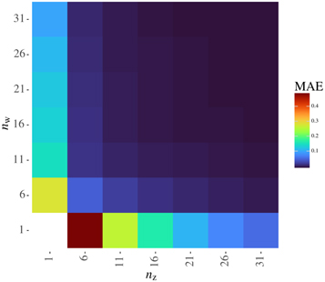
Figure 17. Mean-absolute-error (MAE) for the normalized flux curves for small values of nz and nw. We observe good performance except for the smallest values of nz and nw.
Download figure:
Standard image High-resolution image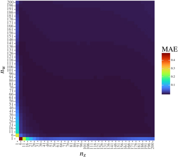
Figure 18. Mean-absolute-error (MAE) for the normalized flux curves for larger values of nz and nw. We observe good performance across the space, with the exception of especially small values of nz and nw.
Download figure:
Standard image High-resolution imageThe figures show that we observe small errors across almost the entire space, with the test set reporting an average MAE of 0.1821 × 10⁻⁶. To put this result into perspective, the average MAE is approximately six orders of magnitude smaller than the mean flux in the training set, which is 0.052 87 Wb. Poorer performance is only observed for small values of nz and nw, particularly when both nz and nw ≤ 6. This behaviour is also observed in figure 19, which shows a selection of ground truth FEA and predicted flux curves for different values of nz and nw. Here we show that for nz and nw ≤ 6 the flux curve model does not make useful predictions, apparently struggling when the magnitude of the flux curve is particularly small. However, for all other cases, the linear model provides an accurate approximation to the FEA curves. Importantly, the model's inaccuracy at particularly small values of nz and nw does not diminish its utility. Coils with nz and nw ≤ 6 correspond to small flux curves with small gradients that do not produce a large emf (and therefore power) as per Faraday's law. As a result, coils with nz ∈ {1, 6} ∧ nw ∈ {1, 6} can simply be excluded from the optimization without affecting the outcome of the optimization process.

Figure 19. A selection of flux curves as obtained using FEA and predicted by our linear model (equation (47)) from the search space for values of nz and nw. The top image (a) shows the normalized flux curves, for comparison purposes. The bottom image (b) shows the flux curves without normalization. We observe a strong agreement in (a) for all examples except for particularly small values of nz and nw, which are associated with flux curves with particularly small magnitudes. (a) Normalized flux curves. (b) Flux curves without normalization.
Download figure:
Standard image High-resolution image7. Optimization
Up to this point, we have developed an electromechanical model in section 3, selected our first category of parameters (parameter that we choose by inspection) in section 4, optimized the our second category of parameters (in order to minimize the difference between the system model predictions and the empirically-measured data) in section 5, and modeled the relationship between the coil parameters and resulting flux curves in section 6. We now turn to the third category of parameters: those that we optimize in order to maximize the power delivered to the load.
The remaining parameters in this third optimization category are given in table 3. They are: the number of coils c, the number of coil windings in the axial direction nz , the number of coil windings in the radial direction nw , the number of magnets m and, where applicable, the coil center distance lccd and magnet center distance lmcd. Note again that all other parameters have either been selected in section 4 or found using empirical data in section 5.
As our objective function, we will maximize the mean power that the microgenerator delivers to a load across a number of input accelerations nacc:


where nt is the number of timesteps.
A visual overview of the optimization process is presented in figure 20. We perform an exhaustive search for each possible combination of parameters c, m, nw, nz and, where applicable, lccd and lmcd, in order to find a combination of optimization parameters that result in a microgenerator design that delivers the most power to the load.
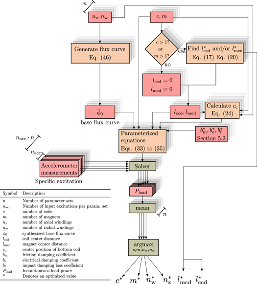
Figure 20. The optimization procedure follows an exhaustive search across all combinations of the values for the parameters nz, nw, c and m that we consider. Using the coil parameters nz and nw, we synthesize a base flux curve  using the linear model in equation (47). If the design involves a multi–coil and/or multi-magnet design, we calculate the optimal spacing between the coils and/or magnets (lccd and lmcd, respectively). We substitute
  , and optionally lccd and lmcd, into the parameterized system of equations represented by equations (33) to (35) that describe the system behaviour, as well as the optimal values found for the mechanical, electrical and impact damping coefficients
  and
and  , respectively in figure 9. The set of parameterized equations is then solved for multiple accelerometer measurements, each solution producing an estimate of the power delivered to the load for the respective input excitation. We select the parameter set that produces the greatest mean power, across all accelerometer inputs, as the best design.
Download figure:
Standard image High-resolution imageFor each parameter combination, we estimate a base flux curve  from coil features nz and nw using the curve model in equation (47). If multiple coils or multiple magnets (i.e. c > 1 or m > 1) are under consideration, then the optimal coil center distance
  and/or magnet center distance
  is also calculated using equations (17) and (20). Next, we calculate the coil center height (cc) of the coil (or the lowermost coil when c > 1) using equation (24). This allows us to compile a parameterized equation set by substituting
  and
and  as well as the best parameter set
  and
and  , found in section 5, into the system model equations equations (33) to (35). The parameterized equation set is then solved for a range of accelerometer measurements (nacc = 15) as input. The accelerometer measurements are taken in an identical way as described in section 5.2.1. The parameterized equation set is solved using the same ODE numerical solver as in section 5.
Each solution produces an estimate for the instantaneous power that the microgenerator will deliver to the load, Pload for a particular acceleration input and parameter set. The result is n = 15 solutions per single parameter set, one for each of the accelerometer measurements. We calculate the mean load power  across this set of solutions, which gives an aggregate estimation of the performance of this particular parameter set and the resulting hypothetical device design. We repeat this process for each possible parameter set of c, m, nw and nz. We select the best design by choosing the parameters that deliver the greatest mean power to the load, denoted as
  and
and  .
.
7.1. Optimization results
We executed the procedure shown in figure 20 for every possible combination of c = {1, 2}, m = {1, 2}, nz = {6, 8, ⋯ ,200} and nw = {6, 8, ⋯ ,200} for a total of npsets = 38416 possible optimization parameter combinations. For the descriptions of these parameters and their effect on the resulting microgenerator design, recall figure 1.
We solve each possible parameter combination for nacc = 15 different accelerometer measurements as input for the acceleration of the microgenerator tube  , resulting in 576 240 solutions total.
We show the mean power delivered to the load  for each optimization parameter combination in figure 21, separated into four 'bins', each representing a different {c, m} grouping. It is evident that values of nz and nw that are too small result in low power output, since the coil captures little flux. Similarly, for nz and nw values that are too large we also observe low power output, since in this case both the rate of change of flux is small (since a large portion of the magnet assembly's magnetic flux is captured by the coil(s) no matter the assembly's relative position) and the total coil resistance matches poorly the load poorly. Between these two extremes, however, there exists an optimum that provides a maximum power output. Furthermore, figure 21 indicates that this optimal point is also the global optimum for a particular {c, m} combination, and that the contour of the resulting load power 'surface' appears smooth. We also see that microgenerators with multiple coils are optimal when coils are shorter (smaller nz) and narrower (smaller nw) than microgenerator architectures with fewer coils. This is likely due to the increased resistance resulting of multiple coil configurations. The optimization also appears to prefer coils that are taller than they are wide (i.e. nz > nw). This is likely due to the particular choice of magnet and its corresponding magnetic field used in our microgenerator architecture.

Figure 21. The mean load power  delivered to a 30Ωload for nacc = 15 accelerometer input excitations, measured using an identical procedure as described in section 5.2.1, for c = {1, 2}, m = {1, 2}, nz = {6, 8, ⋯ ,200} and nw = {6, 8, ⋯ ,200}. The best design for each {c, m} combination is indicated with 'x'. The global best design delivers a mean power of
  for a parameter combination of c = 1, m = 2, nz = 68, nw = 20 and lmcd = 17 mm.
Download figure:
Standard image High-resolution imageWe show the optimal parameter combination, and corresponding power  delivered to the load for each {c, m} combination in table 4. We find that the best configuration delivers a mean power
  to the 30Ωload across all input excitations (n = 15) with parameter combination c = 1, m = 2, nz = 68, nw = 20 and lmcd = 17 mm. Furthermore, we find that the best design delivers slightly more power than for the best c = 2 and m = 2 configuration, suggesting that adding both additional coils and magnets does not always guarantee more power. Figure 21 shows that optimal parameters not only exist, but achieve vastly greater power output than most other designs that we considered in the exhaustive optimization set. As an example, let us consider the c = 1 , m = 1 microgenerator as a 'naive' reference design. Even with the best possible coil parameters for nz and nw, our optimum c = 1, m = 2 devices achieves ≈ 2.8x the load power output of this reference design. Here we note that the 'naive reference' is taken as the optimum c = 1, m = 1 device after optimization. Non-optimal choices of nz, nw leader to even lower output. This demonstrates the benefit of our proposed optimization process.
Table 4. Optimal combination of parameters nz, nw, lccd and lmcd for each combination of {c, m} and the corresponding mean power  , over nacc = 15 input excitations, that is delivered to the 30Ωload.
| c | m | nz | nw | lccd (mm) | lmcd (mm) |
 (W) (W) |
|---|---|---|---|---|---|---|
| 1 | 1 | 72 | 20 | — | — | 0.545 × 10⁻³ |
| 1 | 2 | 68 | 20 | — | 17 | 1.526 × 10⁻³ |
| 2 | 1 | 66 | 14 | 16 | — | 0.454 × 10⁻³ |
| 2 | 2 | 64 | 14 | 16 | 16 | 1.431 × 10⁻³ |
The complete set of design parameters for the optimal microgenerator design is shown in table 5.
Table 5. Design parameters for the optimal microgenerator configuration found as a result of the optimization procedure in section 7.
| Description | Parameter | Value |
|---|---|---|
| Number of coils | c | 1 |
| Number of magnets | m | 2 |
| Coil wire radius (mm) | rc | 0.0715 |
| Coil center position (mm) | cc | 82 |
| Number of axial windings | nz | 68 |
| Approx. coil length (mm) | lc | 9.72 |
| Number of radial windings | nw | 20 |
| Approx. coil thickness (mm) | wc | 2.86 |
| Total coil windings | N | 1360 |
| Coil resistance (Ω) | Rc | 69.06 |
| Magnet length (mm) | lm | 10 |
| Magnet diameter (mm) | wm | 10 |
| Magnet center distance (mm) | lmcd | 17 |
| Tube inner radius (mm) | rt | 5.5 |
| Tube bottom thickness (mm) | lbth | 3 |
| Tube wall thickness (mm) | lth | 1 |
| Load resistance (Ω) | Rl | 30 |
| Microgenerator body length (mm) | lL | 135 |
8. Optimized physical device evaluation
Having found our optimal parameters in the previous section, we now physically construct and test the optimal microgenerator design using the experimental setup already shown shown in figure 12 and described in section 5.2.1. By comparing the output of the physically constructed devices with the results computed as part of our optimization we can assess the accuracy of our model equations, as well as the actual power output produced by our optimal microgenerator device.
Our physical optimal microgenerator is constructed in the same was as the reference devices, described in section 5.2.1. The microgenerator body is 3D-printed using PLA using an additive process, and the coil's wire wound using a slowly-turning speed-controlled lathe. As before, we include an axial groove into the microgenerator body to expose the magnet assembly to the camera. A photograph of the manufactured optimal microgenerator device is shown in figure 22.
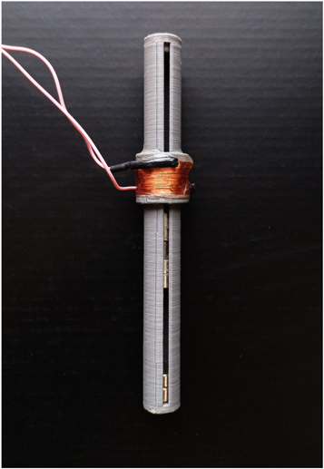
Figure 22. A photograph of the manufactured physical optimal energy harvester, with design parameters given by table 5. The groove reveals the magnet assembly consisting of m = 2 magnets, separated by a spacer, as well as the fixed magnet at the bottom of the device.
Download figure:
Standard image High-resolution imageNext, we followed the same test procedure we used for the references devices in section 5. Measurements were repeated the experiment for ninput = 7 input excitations while measuring the load voltage Vl, the acceleration experienced by the microgenerator body  , and the relative position of the magnet assembly ydiff. The accuracy of our system of model equations equations (33) to (35) was assessed by calculating the same measures prescribed in section 5, only this time for the optimal microgenerator device. These are the normalized Dynamic Time Warping (DTW) distance between the predicted and measured relative magnet assembly displacement
  , the normalized DTW distance between the predicted and measured load voltage values
  and the normalized RMS difference between the predicted and measured load voltage
  .
.
The results for the physical optimal microgenerator device are shown in figure 23, alongside the results calculated for the references devices earlier in section 5. The optimal microgenerator labeled as device O and shown in a separate colour. We can see from figure 23 that our system model is able to predict the behaviour of our optimal microgenerator device with similar accuracy as the reference devices. This indicates that our system model is sufficiently robust to generalize to unseen designs.
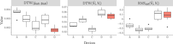
Figure 23. A box-plot distribution estimation, showing the normalized DTW distance between the predicted and measured relative magnet assembly displacement  , the normalized DTW distance between the predicted and measured load voltage
  and the normalized RMS difference between the predicted and measured load voltage
  for the previously-seen reference devices (A, B, C, D) and our optimal microgenerator device (O) found by the optimization process. Notably, the system models predicts the behaviour of the optimal device to a similar degree of accuracy as the reference devices.
Download figure:
Standard image High-resolution imageAdditionally, in figure 24, we show the predicted and measured instantaneous relative magnet assembly displacement ( and ydiff, respectively) in the time domain for the optimal microgenerator device for each of the input excitations. Also here, we observe a high level of agreement, with the model predicting the same dynamics present in the measurements. This corresponds with our earlier aggregate results shown in figure 23. Figure 25 shows the predicted and measured instantaneous load voltage (
 and Vload, respectively) for the optimal microgenerator device for the same input excitations. We again observe a high level of agreement. We believe that this is, at least in part, due to the explicit coupling between the mechanical and electrical aspects of the system of model equations. Notably, we accurately predict both the peak values and waveform shapes, when compared to the ground truth measurements.
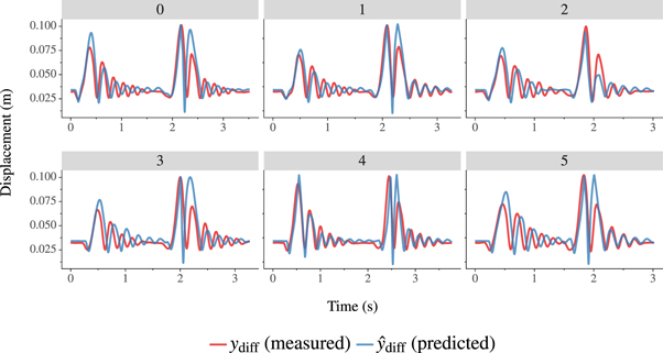
Figure 24. The predicted and measured instantaneous relative magnet assembly displacement for the optimal energy harvesting device across a number of input excitations. We observe a high level of agreement, particularly with regards to the dynamic behaviour.
Download figure:
Standard image High-resolution image
Figure 25. The predicted and measured instantaneous load voltage for the optimal energy harvesting device across a number of input excitations. A high level of agreement is typically observed, particularly with regard to the voltage waveform shape and peak values.
Download figure:
Standard image High-resolution imageIt is noteworthy that this high level of predictive accuracy is possible given the free-form nature of the experimental process (as discussed in section 5.2.1), which results in a high degree of potential variation in the input excitations. This suggests that the system of model equations are general and robust to some significant extent (i.e. not specific to any particular input excitation). The implies is that we could hypothetically apply the process described in this work in the general sense, and use it to design optimal microgenerator devices for arbitrary sources of input excitation. However, despite the positive outlook, further investigation and testing for different applications and microgenerator designs are required to substantiate this claim.
Finally, we assess the benefit of the optimization process with regards to an energy harvester's ultimate goal: powering a load. Using our ground truth measurements and predictions, we compute and compare the predicted and measured power dissipated in the 30Ωresistive load ( and
and  , respectively) for both the reference and optimized microgenerator devices. We calculate the mean load power by taking the RMS of the load voltage over an 8 second period, which encompasses the entire duration of a single input excitation, and then use the RMS to calculate the mean load power using equation (50):

We plot the results in figure 26, which shows the box-plot of the predicted and measured mean load power ( and
and  , respectively) for all reference devices and the optimized microgenerator device. We observe that both the direct measurements and the system of model equations indicate that the optimized microgenerator, O, delivers the most power to the load. What is notable, however, is that the ranking in terms of the power delivered to the load by the system model is identical to that measured in practice.
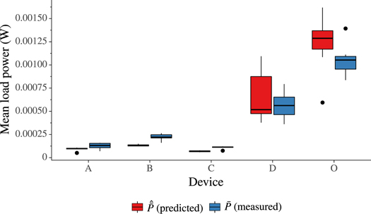
Figure 26. A box-plot showing the distributions of both the predicted and measured mean load power for each reference device, across all input excitations per device. For each measurement, the mean power is calculated over an 8 second time duration. We observe that both the system of model equations and the measurements indicate that the optimized microgenerator, O, delivers the most power to the load.
Download figure:
Standard image High-resolution image
We observe that the system of model equations slightly underestimates the load power for devices A, B, C and slightly overestimates the load power for devices D and O. The definitive cause of this discrepancy is difficult to pinpoint, and could be due to the simplifying assumptions used in the components in the system model equations (33) to (35), inaccuracies in the empirically-derived parameters A, S, bm, be and bf from the parameter discovery process described in section 5, or from inaccuracies in the coil curve prediction model equation (43). These inaccuracies can propagate and accumulate throughout the modelling process. Despite this potential for error accumulation and compounding, the predictions made by the system of model equations remain highly representative of the practical measurements. Figure 26 also demonstrates the practical benefit we derive from the proposed optimization process. The ground truth measurements indicate that, with a measured mean load power of  , the optimized microgenerator O delivers ≈ 8.825x more power to the load than device A, ≈ 4.9x more than device B, ≈ 10x more than device C and ≈ 1.94x more than device D. This is noteworthy when we consider that all the microgenerator devices under test are of similar size and volume. We thus observe that the proposed optimization process is able to produce a microgenerator design that delivers 2–10 times more power to the load than a number of 'naive' reference designs, despite having the same volumetric-budget. Given that the optimization itself is specific to the particular input excitation (and thus can target arbitrary input excitation), we can consider the resulting benefit of the proposed optimization as substantial in application.
9. Conclusion
In this work, we have presented a single-axis microgenerator architecture that consists of a fixed assembly of one or more magnets levitated by a magnetic spring within a tube around which one or more coils are wound. We then proposed a system of model equations that describes the joint mechanical and electrical behaviour of this microgenerator architecture when driven by a particular but arbitrary non-harmonic input excitation. This system model includes a number of different sets of parameters, each determined by means of a different process: the first set is chosen by direct inspection, the second set is optimized to minimize the difference between time-domain predictions and empirical ground truth data, and the third set is optimized in order to maximize the generated power.
The first parameter set, chosen by direct inspection, includes the magnet length lm, magnet diameter wm, the inner tube radius rt, tube wall thickness lth, tube bottom thickness lbth, coil radius thickness rc (and therefore coil resistance per unit length β), coil-magnet gap l
and the target load Rl.
The second parameter set, optimized to minimize the difference between the time-domain prediction of the model and empirical data, includes the mechanical damping coefficient bm, the electromechanical coupling constant be and the mechanical spring damping constant bf, since these are characteristics of the particular physical construction. To determine these parameters for a particular microgenerator architecture, we proposed a method that makes use of an evolutionary algorithm to minimize the difference between the system model's predictions and corresponding ground truth measurements for four distinct real-world reference devices. The measurements in question were the acceleration of the input excitation and the subsequent induced mechanical and electrical behaviour of each reference device. We demonstrated this procedure by means of physical free-form excitation that approximates the motion of a human footstep. The evolutionary algorithm samples different candidate values of bm, be and bf, eventually converging to a set of values that achieves the smallest difference between measured and simulated behaviour. Using the values of bm, be and bf determined in this way, we analyzed the accuracy of the system model and could report a high degree of agreement between the predicted and experimental behaviour of all four reference devices. The predicted RMS load voltage Vload was typically within 25% of the measured value.
Finally, we proposed an optimization process, that can be performed for any input excitation, and that optimizes the final set of parameters c, m, nz and nw to maximize the power delivered to the chosen load. The process consists of a grid search across a range of possible c, m, nz and nw values, where we instantiate the system model using the previously-determined parameters bm, be and bf, and use this to estimate the power delivered to the load. This procedure includes a method that allows the estimation of a flux curve directly from coil properties, since multiple flux curves are required during the optimization. This estimate was achieved using a linear-weighted sum of discrete kernels, and eliminates the need for computationally-expensive FEA simulations. We solved the fully-instantiated system model for 15 different input excitations and selected the parameter set that produced the greatest average load power across all input excitations as the optimal design.
To practically evaluate our computational method, we constructed this optimal device, and tested it using the same footstep-like excitation. We found that this physical realization of the optimal device provided a mean load power of 1.526 × 10⁻³W over the duration of the excitation to a 30Ω target load. This represents a ≈ 2.8-fold increase over the 'naive' single-coil, single-magnet reference device, which served as our baseline. We also found that the system model predicted the behaviour of the optimal device to a similar degree of accuracy as the reference devices, indicating that our system model is a good approximation across a wide range of different energy harvester designs. Moreover, we noted that our system model is able to to correctly rank each device under test according to the power delivered to the load.
We conclude that our proposed system model and associated optimization procedures provide a good approximation to the true mechanical and electrical behaviour of a physically-constructed energy harvester, and that the framework allows the design of an energy harvester providing maximized power output given physical size and weight constraints for specific and non-harmonic input excitation.
Acknowledgments
The authors gratefully acknowledge financial support by the National Research Foundation of the Republic of South Africa and by Telkom South Africa. The authors also gratefully acknowledge the invaluable assistance of Mr Wessel Croukamp and Gift Lecholo in the physical construction of the devices.
Data availability statement
The data that support the findings of this study are available upon reasonable request from the authors.
Declaration of interest
None.