The instrument transfer function for optical measurements of surface topography

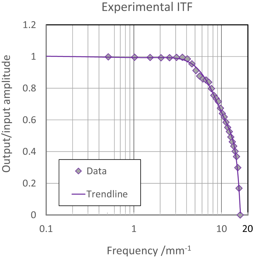
In the development, specification and use of instruments for measuring areal surface topography, a fundamental need is to characterize the expected response to a given surface geometry. It is increasingly common to see graphs similar to that of figure 1, showing the expected measurement results for a sequence of purely sinusoidal surface topography elements of varying spatial frequency [1]. This graph is widely known as the instrument transfer function (ITF). Although the ITF has a standardized definition, its meaning is not always well understood, and methods for evaluating the ITF remain a topic of active research.

Zoom In Zoom Out Reset image size

This paper reviews the definition, use, theoretical modeling, and experimental evaluation of the ITF for topography measuring instruments. The emphasis is on instruments for full-field optical metrology; however, the essential concepts apply to a wide range of contact and non-contact measuring.

'Instrument response' is a general term and can refer to any quantification of the expected results of a measurement. Data interpretations for scatterometry and film thickness analysis, for example, may involve comparing experimental and theoretical signals over a wide range of possible solutions [2–5]. Characterizing the expected response of such instruments often targets a specific measure and surface geometry, such as the dimensions of a periodic test structure having known material properties.

For some applications and measurement methods, it is possible to have a generic specification of instrument response that is independent of the surface geometry. For surface topography, defined as the surface height in the $z$ direction as a function of orthogonal Cartesian surface coordinates $x,y$, the goal is to describe the height variations in terms of basic elements or orthogonal functions. For each of these basic elements, there is a specified response that is characteristic of the instrument. The response to any given surface is then calculated from the sum of the responses to these basic elements.

Suitable functions for a generic characterization of instrument response can be linked to how parts are described and toleranced for manufacture. In the optics industry, for example, this could be Zernike polynomials, asphere coefficients, or Forbes polynomials. A common approach is to use the form, waviness, and roughness ranges for the spatial frequency content of surface topography [6]. Within certain well-defined limits of applicability, knowledge of the spatial frequency response allows for a part-independent approach to characterizing and specifying instrument performance, including the ability to resolve measure closely-spaced surface height features. It is this idea that leads to the concept and definition of the ITF.

In signal processing and control theory, a transfer function (TF) models a device's output for each possible input [7]. In its simplest form, a TF maps an independent scalar input to a dependent scalar output. Most often, TF methods apply to linear time-invariant or spatially shift-invariant systems. For a single variable, the TF for a linear system is an amplifying coefficient plus an optional offset value. Many systems have at least a limited range of input values for which the response can be represented by a linear TF.

In frequency analysis, a TF quantifies the instrument response to sinusoidal basis functions representing the Fourier components of the input. In the frequency characterization of surface topography, we imagine these Fourier components as sinusoidal topography gratings parameterized by surface spatial frequency in the $x,y$ plane and amplitude in the $z$ direction. The ITF catalogs the ratio of output to input amplitude as a function of frequency.

For the ITF curve in figure 1, the ordinate represents the transmission of sinusoidal amplitudes at frequencies noted on the abscissa. For each input frequency, the response maps to the identical output frequency, with a single number representing the ratio of the output (measured) to input (actual) amplitude. At the high end of the frequency range, the instrument reaches a limit of lateral resolution. Similar response curves play a long-established role in dimensional metrology and surface topography characterization [8, 9].

The use of the ITF for optical measurements of surface profiles and areal topographies became common in the engineering and scientific literature in the 1990s. Early work on TFs for 3D measuring microscopes [10] has been followed by techniques that target high-performance applications such as synchrotron optics, photolithography, astronomy and laser fusion [11–14]. The ITF approach has also been applied to structured light projection and other techniques for industrial metrology [8, 15].

Widespread use of the ITF for instrument specification in the last two decades has led to the adoption of the term by the International Organization for Standardization (ISO) [1, 16–18]. The first normative definition for the ITF appeared in the ISO 25178–604:2013 standard for coherence scanning interferometry [19]. The ISO 25178-600:2019 standard, which relates generally to metrological characteristics of all instruments that measure surface topography, defines the ITF as a '...curve describing an instrument's height response as a function of the spatial frequency of the surface topography' [20]. The ISO 25178-600 document further notes that '...ideally, the ITF tells us what the measured height of a sinusoidal grating of a specified spatial frequency would be relative to the true height of the grating.'

Based on the most recent formal ISO definition [20], a mathematical expression for the ITF is

$$\begin{equation}{f_{{\mathop{\textrm ITF}\nolimits} }}\left( \nu \right) = {a_{{\textrm{out}}}}\left( \nu \right)/{a_{{\mathop{\textrm inp}\nolimits} }}\left( \nu \right)\end{equation} \tag{ 1 }$$

where ${a_{\operatorname{out} }},\;\;{a_{\text{inp}}}$ are the output and input amplitudes, respectively, for the spatial frequency $\nu$ of sinusoidal components of the topography. Equations for surface profile components consistent with this definition may be written as

$$\begin{equation}{h_{\text{out}}}\left( x \right) = {a_{\text{out}}}\left( \nu \right)\cos \left[ {2\pi \nu x + {\phi _{\text{out}}}\left( \nu \right)} \right],\end{equation} \tag{ 2 }$$

$$\begin{equation}{h_{\operatorname{inp} }}\left( x \right) = {a_{\operatorname{inp} }}\left( \nu \right)\cos \left[ {2\pi \nu x + {\phi _{{\text{inp}}}}\left( \nu \right)} \right]\end{equation} \tag{ 3 }$$

where ${h_{{\text{out}}}},\;{h_{\operatorname{inp} }}$ are output and input height values in the $z$ direction of the $x,y,z$ coordinate system defined in the ISO 25178-600 standard, and $x$ is a lateral coordinate in the nominal best-fit plane of the surface. The ITF can be defined for any direction in the $x,y$ plane, or if the surface topography is isotropic, it is independent of direction [21].

In the ISO standards and in common usage, the ITF is a positive, real-valued function. For some applications it can be useful to define a Hermitian complex ITF

$$\begin{equation}\widetilde {{f_{\operatorname{ITF} }}}\left( \nu \right) = {f_{\operatorname{ITF} }}\left( \nu \right)\exp \left[ {i\phi \left( \nu \right)} \right]\end{equation} \tag{ 4 }$$

that includes a frequency-dependent phase

$$\begin{equation}\phi \left( \nu \right) = {\phi _{\text{out}}}\left( \nu \right) - {\phi _{{\text{inp}}}}\left( \nu \right)\end{equation} \tag{ 5 }$$

to account for a lateral shift of measured topographical sine waves. In optical instruments, the phase term may be the result of aberrations such as coma that are not symmetrical about the optical axis. A $\pi$ phase shift, equivalent to an inversion of the component profile, is also possible with aliased sampling and image defocus. One also can define a real-valued instrument point spread function (IPSF) that is the inverse Fourier transform of the complex ITF. Prediction of instrument response then relies on convolving the IPSF with the known object surface topography.

Importantly, the ITF for topography measurement is defined in a completely general way that has no direct connection to a specific measurement method or technology. The ISO 25178-600 definition is intended to apply to contact and non-contact instruments, independent of implementation or measurement principle, provided that the measurement is at least approximately linear and invariant over the field of view within well-defined limits.

In the literature, the ITF has many synonyms, including the height TF [17], the system TF [12], the interferometric phase TF [22], composite optical TF (OTF) [11], and the modulation TF (MTF) [23]. The easy misinterpretation of these terms argues for the adoption of the ISO definition to reduce confusion in the meaning and measure of the ITF.

Optical imaging has a long history of frequency analysis, beginning with Abbe's work on diffraction and limiting apertures to define spatial frequency limits of microscopes [24]. Modern Fourier optics is founded on the use of linear systems theory and TFs [25]. It is natural to consider these concepts when evaluating the ITF in full-field optical metrology.

For incoherent light, imaging instruments are characterized by the linear MTF, which describes the contrast of imaged intensity patterns as a function of spatial frequency [26]. Typically, the MTF declines with spatial frequency, eventually reaching a limit according to the resolving power of the instrument.

The ISO 9334:2012 standard defines the MTF as the magnitude of the complex-valued OTF, which itself is the Fourier transform of the real-valued incoherent point spread function (PSF) [26, 27]. In this definition, the PSF and the MTF relate only to the optics in an instrument—that is, the optical components, limiting apertures, and illumination. When specifying instrument performance for the complete measurement process, the definition is often extended to a system MTF, which includes electro-optical components and data processing [26, 28]. Although the term 'MTF' is frequently used as a synonym for the system MTF, they are of course not the same and some care is necessary to avoid confusion. As a case in point, if the image is recorded using an electronic camera, the spacing, size, and detection characteristics of the imaging pixels influence the system MTF, resulting in an instrument response that can be very different from the purely optical MTF [26].

For surface topography measurements, the ITF is defined in the ISO standards without reference to the system MTF for optical imaging. As has been noted, the intent of the ITF is to describe the complete process of generating areal surface topography maps, independent of the instrument type. Optical topography measurement involves diverse principles, including focus effects, triangulation, time of flight, and interferometry to detect differences in surface heights. While the filtering properties of optical imaging systems play a role in determining instrument response, the ITF for optical techniques can be similar to or entirely different from the system MTF for conventional imaging.

Interferometry can be a useful example to highlight the differences between the ITF and the system MTF. Interferometers use the phase and sometimes the contrast of interference patterns to determine surface topography [29]. While in many cases the imaging of interference fringes may be a linear process, the same linear filter does not necessarily apply to the final topography measurement. It can happen that the ITF and the system MTF are similar, as has been demonstrated for phase-measuring interferometry for surfaces in the limit of small surface height variations [16]. However, this is by no means the case in general. The instrument response of many practical interferometers is not well represented by the system MTF, even for small range of surface heights [29–31].

When the ITF is different from the system MTF for conventional imaging, there are aspects of the MTF that are still relevant to the ITF. The upper frequency limit to the MTF, corresponding to the Abbe limit, is a useful milestone for the highest detectable spatial frequency for optical imaging given the limiting apertures in the optical system [32, 33]. Similarly, the related Rayleigh and Sparrow limits for closely-spaced surface features are commonly-used specifications of optical lateral resolution for instruments that measure surface topography [20]. Although it is certainly possible to detect and quantify surface structures beyond this limit, for example by solving the inverse problem with some prior knowledge [34]; the resolving power for surface topography over the linear response range of the instrument corresponds closely to the traditional high-frequency limits of the MTF [35].

The MTF is defined for incoherent optical imaging of intensity patterns. For coherent imaging, the OTF is replaced by the amplitude TF, which is linear in light amplitude, rather than in light intensity [25]. Consequently, there is no standardized or commonly-understood meaning to an MTF for coherent or partially-coherent imaging. Interestingly, interferometers can have the property that optical filtering of imaged interference patterns can be represented by a linear TF over a continuum of illumination conditions, from spatially coherent to incoherent [36, 37]. However, this is not generally the case for optical instruments, which must be analyzed according to their specific principles of measurement.

To summarize this section, the MTF for optical imaging may contribute to the ITF for topography measurements, but the MTF and the ITF are most definitely not the same thing. To determine the ITF, even if the MTF is known, we require modeling of the complete measurement process or an experimental measurement of ITF using an appropriate set of sample parts.

Predicting the frequency response of an instrument using theoretical modeling involves a sequence of numerically simulated test patterns over a spatial frequency range of interest [36, 38]. Evaluation of the frequency response for nonlinearity and dependence on sinusoidal amplitude determines under what conditions an ITF specification is meaningful, as well as the final ITF curve.

This section first describes a general procedure for quantifying instrument response as a function of isolated sinusoidal topography patterns. This is followed by a specific example for a phase-shifting interference microscope with a partially coherent, monochromatic light source. It will be shown that the instrument response follows a clear trend of declining amplitude transmission with increasing frequency; however, the rate of decline depends on the maximum surface slope present in the sinusoidal patterns. For the purpose of instrument specification, the ITF for instruments of this type can be defined in the limit of small surface slopes. For higher slope values, the ITF concept is still useful, with the understanding that there is a quantifiable degree of part dependence and nonlinearity. This example serves to illustrate how instrument simulations can assist in the determination of the ITF and its range of validity.

The example calculation of instrument response begins with a sinusoidal profile as defined by equation (3):

$$\begin{equation}{h_{\operatorname{inp} }}\left( x \right) = {a_{\operatorname{inp} }}\left( \nu \right)\sin \left( {2\pi \nu x} \right),\end{equation} \tag{ 6 }$$

where the phase term ${\phi _{\operatorname{inp} }}$ has been set to $\pi /2$ and the lateral coordinate range is

$$\begin{equation} - L/2 < x \le - L/2\end{equation} \tag{ 7 }$$

for a field of view width $L$. The frequencies $\nu$ are integer multiples of $1{\textrm{/}}L$ so that ${h_{\operatorname{inp} }}$ is zero at the boundaries of the field of view, to avoid edge effects.

After simulating the corresponding output profile ${h_{\text{out}}}$ using any appropriate instrument model, the measured amplitude ${a_{\text{out}}}$ follows from a fit of a sine wave at the fixed frequency $\nu$, with an adjustable amplitude ${a_{\text{out}}}$ and phase shift ${\phi _{{\text{out}}}}$. An appropriate fitting function is

$$\begin{equation}{h_{{\text{fit}}}}\left( x \right) = \operatorname{Re} \left\{ {\widetilde {{a_{\text{out}}}}\left( \nu \right)\exp \left( {i2\pi \nu x} \right)} \right\}\end{equation} \tag{ 8 }$$

with a complex amplitude

$$\begin{equation}\widetilde {{a_{\text{out}}}}\left( \nu \right) = {a_{\operatorname{out} }}\left( \nu \right)\exp \left[ {i{\phi _{{\text{out}}}}\left( \nu \right)} \right].\end{equation} \tag{ 9 }$$

The best-fit result is for

$$\begin{equation}\widetilde {{a_{out}}}\left( \nu \right) = \frac{1}{L}\int\limits_L {{h_{out}}\left( x \right)\exp \left( { - i2\pi \nu x} \right){\text d}x} .\end{equation} \tag{ 10 }$$

The frequency response independent of the phase shift is determined from the modulus ${a_{\operatorname{out} }}$:

$$\begin{equation}{f_{{\textrm{FR}}}}\left( \nu \right) = {a_{{\textrm{out}}}}\left( \nu \right)/{a_{{\mathop{\textrm inp}\nolimits} }}\left( \nu \right).\end{equation} \tag{ 11 }$$

The fit is equivalent to Fourier analysis. As an option, the phase shift $\phi$ for use in the complex-valued ITF is

$$\begin{equation}\phi \left( \nu \right) = {\phi _{{\textrm{out}}}}\left( \nu \right) - \pi /2.\end{equation} \tag{ 12 }$$

The frequency response ${f_{{\text{FR}}}}$ can be equivalent to the function ${f_{{\text{ITF}}}}$ as defined by equation (1), provided that the results are consistent with the definitions of the ITF. Part of this evaluation is a determination of how well a simple scaling of the sinusoidal amplitude by the response function ${f_{{\text{FR}}}}$ predicts the measured profile. In a realistic simulation, the output profile is unlikely to be perfectly sinusoidal, because of inherent imperfections and nonlinearities in the measurement process. These imperfections can be quantified for each frequency $\nu$ as a relative residual error profile

$$\begin{equation}\varepsilon \left( x \right) = \frac{1}{{{a_{{\text{inp}}}}}}\left[ {{h_{\text{out}}}\left( x \right) - {h_{{\text{fit}}}}\left( x \right)} \right].\end{equation} \tag{ 13 }$$

This difference profile can be reduced to a single parameter for summarizing the magnitude of residual errors. A simple approach that assumes no outliers or spurious data points is to calculate the root-mean square deviation

$$\begin{equation}{\varepsilon _{{\textrm{RMS}}}} = {\textrm{ }}\sqrt {\frac{1}{L}\int\limits_L {{\varepsilon ^2}} \left( x \right){\textrm{d}}x.} \end{equation} \tag{ 14 }$$

If the measurement task assumes linearity in spatial frequencies, these residuals are a contribution to the topographic fidelity—a metrological characteristic defined in ISO 25178-600:2019 [20].

The frequency response simulation can be carried out for a constant amplitude ${a_{\operatorname{inp} }}$ for all frequencies $\nu$. However, given the slope limitations for optical systems, it can be more useful to calculate the response with a fixed maximum slope angle $\gamma$ instead of a fixed sinusoidal amplitude [36, 39]. The amplitudes are

$$\begin{equation}{a_{{\textrm{inp}}}}\left( \nu \right) = \tan \left( \gamma \right)/2\pi \nu .\end{equation} \tag{ 15 }$$

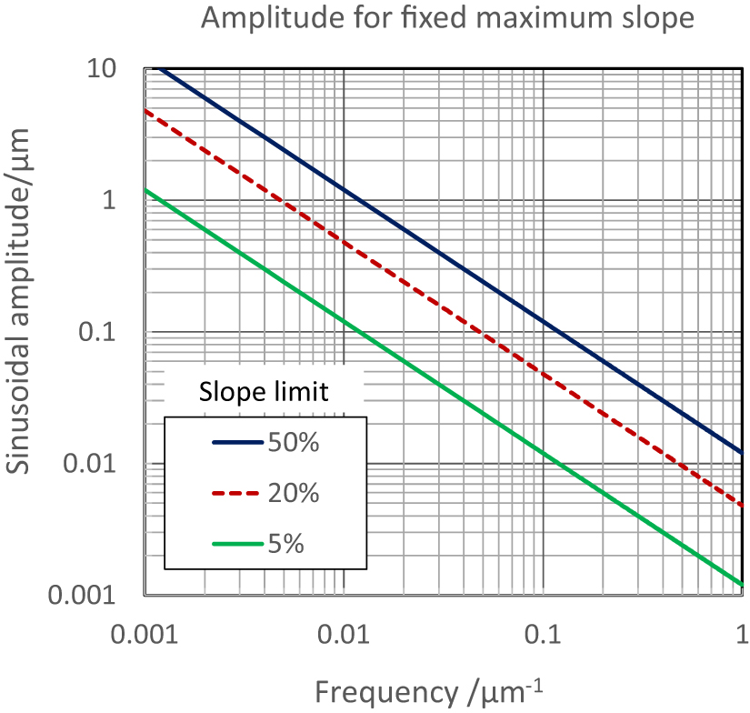
The usual guidance is to have surface slopes well below the geometrical angle limit $\beta$defined by marginal ray paths through the optical system. For microscopes using incoherent Köhler illumination with a common aperture for both illumination and imaging, the sine of the angle $\beta$ in air is approximately equal to the numerical aperture (NA) of the objective [20, 40]. Figure 2 illustrates the resulting range of amplitudes for an NA of 0.15, for three slope limits defined by the ratio $\gamma /\beta$. The lateral spatial frequency range extends from a single sinusoid over a 1 mm field of view to a 1 µm spatial period. An amplitude distribution that declines with spatial frequencies is consistent with realistic surface geometries that have larger height variations at low frequencies than at higher frequencies.

Zoom In Zoom Out Reset image size

Methods for simulating optical measurements include advanced solvers for surface features with high-aspect ratios [41], structured surface films [42], dissimilar materials [43], field-focus effects [44], and surface slopes beyond the aperture limits of the instrument [45]. For smooth sinusoidal profiles with height variations less than the depth of field, a classical Fourier optics imaging model is adequate and is a computationally efficient approach [25, 36, 46].

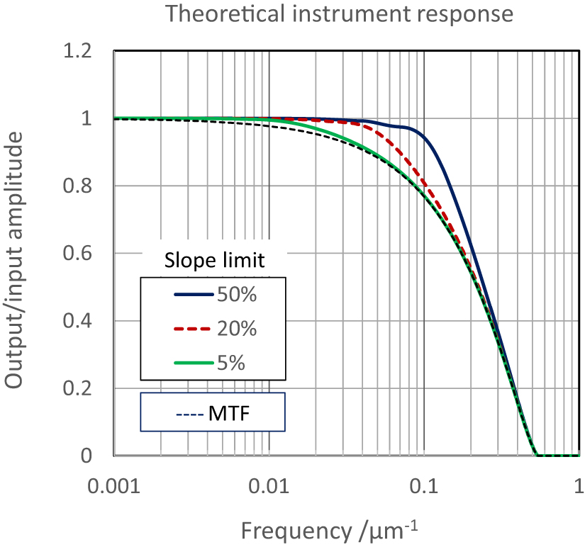
Figure 3 shows results for a phase-shifting, monochromatic interference microscope with an objective NA of 0.15 and an illumination pupil filled with 0.55 µm incoherent light, calculated using a classical Fourier optics model [36]. The amplitude inputs are plotted in figure 2. For comparison, the graph includes the theoretical MTF for incoherent imaging of intensity patterns.

Zoom In Zoom Out Reset image size

For the 5% slope limit in figure 3, the frequency response is nearly identical in functional form to the imaging MTF, consistent with previous studies [16]. The relative residual error shown in figure 4 is less than 0.25% over this frequency range. For the maximum slope limit values of 20% and 50% corresponding to higher surface topography height variations, the response shown in figure 3 is greater than the MTF for spatial frequencies from 0.01 $\mu {{\text{m}}^{ - 1}}$ to 0.2 $\mu {{\text {m}}^{ - 1}}$. This enhanced response has been verified experimentally (see [36]). However, figure 4 shows that there are also larger residual errors at these slope limits. Figure 5 shows the residual error at the peak frequency of $\nu = 0.08\,\mu {{\text{m}}^{ - 1}}$ and a sinusoidal amplitude ${a_{{\text{inp}}}} = 0.14\,\mu {\text{m}}$. The distortions are harmonics of the fundamental frequency.

Zoom In Zoom Out Reset image size

Zoom In Zoom Out Reset image size

The results in figure 3 show how the instrument will respond to single-frequency sinusoidal profiles; however, the response varies with slope limit, and there is the potential for error as shown in figures 4 and 5 if it is assumed that the measurement results are predictable using an ITF. These discrepancies are minimized for small surface slopes and height variations, consistent with the known limits of ITF characterization for optical instruments, as described in the literature [16, 40] and in the ISO 25178-604:2013 standard [20]. Consequently, for the purpose of specifying instrument performance under favorable conditions, a meaningful approach is to use the 5% slope limit in figure 3 for the ITF curve.

For the higher slope limits in figure 3, it is reasonable to refer to these response curves as 'approximate' or 'apparent' ITFs. This is common practice, although not always with the appreciation that these curves may not accurately predict the response to a random surface profile using simple linear TF methods.

For all three curves in figure 3, the maximum detectable frequency of $\nu = 0.55\,\mu {{\text{m}}^{ - 1}}$ is the Abbe frequency limit, given by

$$\begin{equation}{\nu _{{\textrm{Abbe}}}} = 2{A_{\textrm{N}}}/\lambda ,\end{equation} \tag{ 16 }$$

where ${A_{\text{N}}}$ is the NA. This observation shows that at least for this example, the ultimate resolving power of the instrument is unchanged by the surface slopes and departures.

The ITF describes the response of the complete system, including the detection system, which in full-field methods is most often a digital camera. The size of the individual pixels in object space—the magnified or reduced image size of the pixel on the object surface—can be a significant contributor to the ITF, especially for large fields of view for which the optical lateral resolution is comparable to the lateral sampling interval of the camera. The calculation of the ITF contribution from pixel size is straightforward [26, 47], and for many cameras it is sufficient to assume that the width of the integrating area of the pixel is the same as the lateral sampling interval $D$ at the object surface. The multiplicative contribution of the pixel size to the ITF is

$$\begin{equation}{f_{{\text{CAM}}}}\left( \nu \right) = \frac{{\sin \left( {\pi \nu D} \right)}}{{\pi \nu D}}.\end{equation} \tag{ 17 }$$

This function has zeros for frequencies $\nu$ that are integer multiples of $1/D$.

Figure 6 shows the TF for two object-space pixel widths, 1 µm and 10 µm. These values are for two different magnifications with the same camera, the difference being the magnification from object to image. Ideally, optical instruments are designed such that the pixel spacing is much smaller than the optical PSF. However, especially at low magnifications, it can be the case that the system is 'pixel limited' and it is important to consider the pixel width as part of an ITF prediction. It can also happen that the camera pixels are not fully independent, resulting in a decline in instrument response with frequency that is dominated by the camera, even when the high-frequency lateral resolution limit is unchanged. This effect is common in some kinds of complementary metal–oxide–semiconductor (CMOS) imagers.

Zoom In Zoom Out Reset image size

For the frequency response curves in figure 6, the camera transmission falls to zero at twice the Nyquist sampling limit, corresponding to one sinusoidal cycle over a lateral distance of interval $2D$. The response then rises and falls periodically with every $1/D$ increase in frequency. Values above the Nyquist frequency correspond to aliasing of high-frequency sinusoids beyond the sampling abilities of the camera. Aliasing results in coupling of high frequencies to low frequencies, which is inconsistent with the definition of a linear, frequency-domain TF. For this reason, optical magnification should be chosen so as to avoid aliasing by having pixel spacings in object space well below the optical lateral resolution [26].

Real optical systems are not perfect and have a variety of imperfections and aberrations [38, 48]. Even a well-designed instrument can struggle to achieve the theoretical ITF for diffraction limited imaging because of setup issues, including focus errors. Figure 7 compares theoretical in-focus and out-of-focus ITF curves for an NA of 0.15, a wavelength of 0.55 µm and the 5% slope limit shown in figures 2 and 3, using Fourier optics modeling [36]. These curves show that defocus degrades the ITF and blurs the sinusoids. Figure 8 shows that focus errors also increase the residual error as calculated by equation (14) even in the limit of small surface heights.

Zoom In Zoom Out Reset image size

Zoom In Zoom Out Reset image size

The defocus of 10 µm is large for a microscope, but it is a possibility when setting up a single-wavelength system. The defocus attenuates the response to zero at a frequency of $0.3\,\mu {{\text{m}}^{ - 1}}$; but the ITF rises again before falling again to zero just below the Abbe limit of $0.55\,\mu {{\text{m}}^{ - 1}}$. The response with defocus above $0.3\;\mu {{\text{m}}^{ - 1}}$ has a π phase shift for ${\phi _{\text{out}}}$. However, unlike camera sampling effects, high frequencies are not aliased to lower values. This can make it difficult to determine the best focus position when setting up single-wavelength instruments such as laser Fizeau interferometers, because out-of-focus measured profiles can have sharp features characteristic of a high spatial frequency response. This problem has motivated the development of automated focusing methods based on holographic propagation [49].

As practical guidance for measurement systems such as fixed-focus PSI, minimizing the effect of focus errors on the ITF requires that all measured points be well within the depth of field given by the Rayleigh formula

$$\begin{equation}{D_{{\text{field}}}} = \pm \lambda /A_N^2.\end{equation} \tag{ 18 }$$

It can also be useful to apply modeling methods as has been done here, using open-source software simulators provided by researchers and instrument makers [50].

For instruments that perform axial scanning, such as coherence-scanning microscopes [29], the part setup is less of a focus issue; however, the instrument itself can have focus errors. These can arise for example from a difference in the position of best focus and the position of highest fringe contrast [44].

The theoretical ITF results presented here do not include any post processing that alters or limits the spatial frequency content of the measurement. In practice, it is common to filter measured topography to emphasize frequency scales of interest [9, 51]. In the specification of ITF for targeted applications, it is essential to account for any applied smoothing or bandpass filters.

A logical question related to the ITF is whether the instrument response can be made more uniform up to the high-frequency limit by applying a frequency-domain filter proportional to the inverse of the ITF, or equivalently, by a deconvolution algorithm [13]. This can have the effect of enhancing the apparent resolving power of the instrument, especially if the lateral resolution is defined in terms of an ITF value such as the frequency for which the ITF falls to 50%. The caution is that amplification of the response at high spatial frequencies to enhance the ITF also amplifies the measurement noise at these frequencies [52].

Post-processing can also correct anomalies and inconsistencies in the ITF. As an example, a default high-frequency attenuating filter compensates for the exaggerated sensitivity of some optical techniques to sharp-edged surface features [53]. Further, although it is not common, iterative post-processing can reduce the dependency of the frequency response to surface slopes, so as to extend the usable range of ITF methods.

Instrument modeling is an important part of ITF evaluation; but even the best model requires experimental validation, using a technique that allows for empirical calculation and ideally, traceable calibration of the frequency response.

The traditional calibration framework for dimensional metrology is by means of 'material measures' or 'etalons', defined in the International Vocabulary of Metrology as the '...realization of the definition of a given quantity, with stated quantity value and associated measurement uncertainty, used as a' [54]. Material measures enable traceability by comparisons with physical specimens certified via reference metrology [55]. Familiar material measures include step height specimens for calibration of the amplification coefficient (height-scaling factor) [56, 57]. The ISO 25178-70 document defines an assortment of material measures for basic calibration of areal surface topography measuring instruments [57, 58].

There is to-date no normatively defined material measure for the ITF. This is in large part attributable to two factors: The need to provide sample structures tailored to the linear operating range of each specific measurement method and the cost and difficulty of manufacturing and certifying appropriate material measures. Consequently, there is a range of sample types and evaluation methods for empirically determining the ITF of full-field optical measuring instruments [59].

The most appropriate set of material measures for the ITF is an ensemble of certified sinusoidal gratings over a range of amplitudes and frequencies that fit between the measurement noise limits on the one hand and the maximum surface slope limits on the other [60]. For direct quantification of the ITF independent of the measurement technology, this remains the ideal method.

A variety of material measures have been proposed to simplify the collection of ITF information without relying on what can be an impractically large number of individual sinusoidal topography samples. An approach is to provide gratings that have a constant amplitude and frequency chirp as a function of lateral position [61]. The Physikalisch-Technische Bundesanstalt has fabricated high-quality material measures of this type using an ultra-precision lathe [62]. Alternatively, as has been noted above in the context of ITF modeling, many instruments have response limits that are most closely related to surface slope. This can be addressed by having the amplitude of the grating decrease as the frequency increases, as recommended in section 6 for ITF evaluation using simulated surface structures [39]. However, even with this improvement, a set of samples are required to accommodate slope limits that vary with magnification and aperture limits.

In addition to the inconvenience of requiring a set of material measures of varying sinusoidal amplitude and frequency to determine ITF, it is difficult and expensive to fabricate and to certify purely sinusoidal gratings, with the consequence that ITF calibration is rarely performed this way in practice. Manufacturing challenges have motivated the development of material measures based on periodic rectangular or binary profiles created using lithographic technology. Rectangular profiles are analogous to grill patterns in imaging MTF analysis [63]. Figure 9 illustrates an example of this approach [64, 65]. Recent progress includes the design and fabrication of high-quality circular patterns with chirped frequency and surface height variations within the linear ITF range of optical instruments [21].

Zoom In Zoom Out Reset image size

A material measure having similar functionality to a chirped rectangular-profile grating is a Siemens-star pattern, which also has analogous patterns in imaging MTF analysis [66]. These patterns are especially convenient for identifying specific response levels along the ITF curve, including the lateral period limit, defined as the 50% response point on the curve [67].

Lithographic methods enable the creation of binary pseudo-random arrays comprised of rectangular surface features of varying lateral dimensions distributed throughout the field of view. These arrays can be designed to allow for a direct determination of the ITF with uniform sensitivity over the full spatial frequency range and field-of-view of an instrument, with high signal to noise [23]. This approach has recently been advanced with the development of isotropic 2D arrays [68].

The ease of fabrication of rectangular profile ITF samples compared to other designs comes at the price of not adhering to the concept of analyzing frequency response using pure sinusoidal topographies. A rectangular profile also complicates the evaluation of residual nonlinearities (equation (13)) as a means of objectively establishing confidence in the ITF representation of instrument response. The rectangular profiles run the risk of introducing multiple scattering, interferometric fringe-order errors, or other nonlinear phenomena. For these reasons, rectangular profile material measures are often regarded as serving a dual purpose—determining frequency response while at the same time challenging the ability of a candidate technology to successfully measure difficult structures [69, 70]. This is particularly the case if the edge features are larger in height than an eighth of the wavelength of the source light [16]. Recent work has advanced methods to analyze the instrument response to challenging surface structures, including those that result in outliers [62, 69, 71].

An alternative to periodic grating-like topographies for ITF evaluation is to determine the IPSF defined in section 4 as the Fourier transform of a complex representation of the ITF. Determining the IPSF experimentally requires an object that generates an impulse response in the topography measurement. Ideally, this would be a sphere or needle tip having a radius much smaller than the anticipated width of the IPSF in object space. An alternative is to provide spheres of well-characterized shape and just a few tens of micrometers in radius, for example, from the formation mercury sessile drops [57, 72]. While this approach is not yet common practice, it has the appeal of just one measurement to determine the ITF, calculated from the magnitude of the forward Fourier transform of the IPSF.

In place of a small sphere or needle tip, a more widely-adopted method for approximating the IPSF is to evaluate the instrument edge spread function (IESF) for a profile along one surface coordinate, for example the $x$ axis, using a sharp step-height feature [73]. This technique is similar to imaging MTF analysis using the response to a high contrast knife edge [74]. For surface topography, the step feature should be sufficiently high so as to provide data above the measurement noise level, but small enough to avoid nonlinear behavior [16, 65, 73]. For interferometry, a suitable step height is approximately one tenth of the source wavelength.

Often it is sufficient and practical to use step-like material measures intended for calibration of the instrument scales to perform the IESF test for ITF evaluation. However, even customized single step height features are much easier to fabricate than gratings, and no calibration or certification of the step height is required—the analysis is based on the frequency content of the derivative of the measured step, normalized by the value at zero frequency [63]. Figure 10 shows the image of a sample part with etched 38 nm steps for ITF analysis of laser Fizeau interferometers [65]. This was the measurement method used to create figure 1 in the introduction.

Zoom In Zoom Out Reset image size

Although isolated step features are convenient, they are not without their drawbacks. The flat substrates must be exceptionally well polished prior to etching to avoid spurious topographical frequencies, and the sharpness of the step should be verified using metrology with higher resolution and fidelity than that of the final ITF test setup. The Fourier components of a step feature decline in amplitude with frequency, potentially leading to inadequate signal to noise level at high spatial frequencies. Finally, this approach shares with other methods the disadvantage complicating evaluation of frequency mixing and residual errors by presenting the instrument with a range of spatial frequencies simultaneously.

An indirect approach to ITF evaluation relies on empirical methods to evaluate the key contributing factors to an ITF prediction using an instrument model [75]. For optical instruments, a key contributor is the spatial filtering characterized by the OTF and the corresponding system MTF. As a simple example, we can take advantage of the approximate equivalence of the system MTF and the ITF for small surface height variations (see section 5). In figure 11, the experimental MTF curve for an interference microscope follows from the imaging edge spread function using a cleaved silicon wafer [74]. The ITF curve is for a topography edge-spread function obtained with a 0.04 µm topographical step height. For this specific example, it is sufficient to evaluate the MTF experimentally to determine the final ITF of the instrument. This approach can be extended in principle to coherent light and aberrated optical systems where the ITF is not directly equivalent to the system MTF [75, 76].

Zoom In Zoom Out Reset image size

Once we have a reliable ITF curve, obtained either through simulation or experiment, the results indicate measurement capability for specific targeted applications.

Perhaps the most common use for the ITF is in qualifying instruments for the measurement of the power spectral density (PSD). The PSD is defined in ISO 10110–8:2010 as the square magnitude of the Fourier transform of the surface heights along one dimension, after removal of the low-order surface form [6]. In terms of the previously-defined amplitudes $a_{{\text{inp}}}^{},a_{{\text{out}}}^{}$, the object surface PSD is

$$\begin{equation}{P_{{\text{inp}}}}\left( \nu \right) = a_{{\text{inp}}}^2\left( \nu \right)\end{equation} \tag{ 19 }$$

while the measured value is

$$\begin{equation}{P_{{\text{out}}}}\left( \nu \right) = a_{{\text{out}}}^{\text{2}}\left( \nu \right).\end{equation} \tag{ 20 }$$

Consequently,

$$\begin{equation}{P_{{\text{out}}}}\left( \nu \right) = f_{{\text{ITF}}}^{\,2}{P_{{\text{inp}}}}\left( \nu \right).\end{equation} \tag{ 21 }$$

PSD specifications control the quality of optical components and transmitted wavefronts, particularly for mid- and high-spatial frequencies [11, 12, 14, 77].

The PSD of most surfaces allows for larger surface height variations at low frequencies compared to higher frequencies. Figure 12, for example, illustrates a PSD specification for the surface finish of high-quality optics. This trend is consistent with the constant slope limit method of evaluating the ITF, as illustrated in figure 2.

Zoom In Zoom Out Reset image size

Of importance is that the PSD is a power density, corresponding to the square of the sinusoidal surface height variations over a range of frequencies, hence the units of square nanometers times micrometers in the figure. An important property of the PSD is that the normalized integration of the PSD over a range of frequencies provides the mean-square deviation of the surface profile for the scale-limited surface. In Fourier analysis, the minimum frequency range or 'bin size' is determined by the sampling length.

The PSD example in figure 12 covers a range of spatial periods from 1 mm to 1 µm. To evaluate conformance to this specification would almost certainly require more than one measurement, using different magnifications to manage the lateral sampling requirements, and different NA values to balance field of view with optical resolution [78, 79]. In PSD evaluations over larger frequency ranges, more than one instrument type may be needed, for example, a laser Fizeau, an interference microscope, and an atomic force microscope. The resulting measurements can be normalized by their ITF values over specific frequency ranges to piece together a complete picture of the surface characteristics as quantified by spatial frequency content.

A more ambitious use for the ITF is to predict complete measured topographies, as opposed to quantifying their frequency content alone in a PSD. For this, the lateral shifts $\phi$ in the sinusoidal basis functions of the surface decomposition should be included in the complex-valued ITF defined by equation (4). The measured topography is then an integral over all relevant frequencies

$$\begin{equation}{h_{out}}\left( x \right) = \int {\widetilde {{a_{out}}}\left( \nu \right)\exp \left( {i2\pi \nu x} \right)d\nu } \end{equation} \tag{ 22 }$$

where the complex-valued output amplitudes are

$$\begin{equation}\widetilde {{a_{{\text{out}}}}}\left( \nu \right) = \widetilde {{a_{{\text{inp}}}}}\left( \nu \right)\widetilde {{f_{\operatorname{ITF} }}}\left( \nu \right)\end{equation} \tag{ 23 }$$

and the input amplitudes are the Fourier components of the surface topography

$$\begin{equation}\widetilde {{a_{{\text{inp}}}}}\left( \nu \right) = \frac{1}{L}\int_L^{} {{h_{{\text{inp}}}}\left( x \right)\exp \left( { - i2\pi \nu x} \right){\text d}x} .\end{equation} \tag{ 24 }$$

An ITF analysis is also a viable approach to quantifying topographical fidelity, by a systematic determination of the instrument response for the spatial frequency content of sample parts to be measured. This is particularly the case when the response deviates strongly from an ITF model as the result of slope effects, nonlinear behavior or spatial frequency mixing. Instrument models in the published literature highlight the kinds of surface structures that may require guidance from instrument makers and measurement experts to optimize the results [36, 80]. A caution is that modern instruments often have proprietary hardware and software specifically designed to enhance measurement fidelity—a reality that argues in favor of further developments in standardized specimens as well as calibration techniques for determining the metrological characteristics of a given instrument [81].

While there are many benefits to ITF characterization, it is not always the most effective way to characterize an instrument. The response of contact stylus instruments, for example, is more realistically modeled as a morphological filter based on a structuring element such as a rolling ball, to emulate the effect of the physical dimensions of the stylus tip [82]. Similarly, for optical instruments, there are many useful applications for machined or additively manufactured surfaces for which the results are not well represented by a linear, frequency-domain ITF [83, 84]. There is active research into virtual instrument models that can be more flexible and accurate predictors of measurement results and associated uncertainties [80].

Notwithstanding the limitations of the ITF, many manufacturing processes are controlled by surface quality specifications closely tied to surface frequency analysis. ITF characterization is a much more complete and informative representation of optical instrument response than a simple statement of lateral resolving power, such as the Rayleigh or Sparrow limit. The ITF quantifies the response of the instrument to specific spatial frequencies, and at least in principle, provides a means to predict the measured result for an arbitrary surface structure using linear transform methods, within well-defined limitations of applicability. Looking forward to further research, there is the potential for extending the ITF concept beyond surface metrology to a full 3D frequency response to accommodate data from tomographic images with data structures that represent volumetric data [85, 86].

Given these benefits, it is likely that the ITF will continue to be an important way to characterize the capability of full-field optical metrology systems and methods.

I would like to thank Xavier Colonna de Lega, Leslie Deck, and Shiguang Wang at Zygo Corporation for their contributions to this work. I would also like to thank Richard Leach and Rong Su at the University of Nottingham, and Han Haitjema at the University of Leuven, for their careful review of the manuscript and many useful discussions.