Abstract
Impurity particles (slime particles) play a vital role in copper electrorefining, as they are a major source of cathodic contamination. Their behavior and transport in electrorefining cells are largely affected by electrolyte flows. Therefore, it is significant to study the fluid flow field in copper electrorefining with the consideration of impurity particles. A two-phase flow model of copper electrorefining was developed with one liquid phase of electrolyte and one dispersed phase of impurity particles. Copper electrorefining in a lab-scale cell was then simulated for two different impurity particle releasing scenarios. With impurity particle released only from the inlet, dispersed phase particles can be transported to the inter-electrode domain by electrolyte inflows through its sides rather than its bottom. Thus, the side parts of the cathode encounter more impurity particles than the center part in this scenario. With impurity particles released from both the inlet and the anode, dispersed phase particles fill up the electrorefining cell much faster, and the cathode is exposed to significant volume fractions of the dispersed phase much earlier. A large amount of impurity particles from the anode are settled on the cell bottom. The dispersed phase particles are distributed almost uniformly in front of the cathode after initial stages.
Export citation and abstract BibTeX RIS

This is an open access article distributed under the terms of the Creative Commons Attribution Non-Commercial No Derivatives 4.0 License (CC BY-NC-ND, http://creativecommons.org/licenses/by-nc-nd/4.0/), which permits non-commercial reuse, distribution, and reproduction in any medium, provided the original work is not changed in any way and is properly cited. For permission for commercial reuse, please email: oa@electrochem.org.
Copper electrorefining is widely applied in the world to produce Grade-A copper (>99.99%) that can be further processed to make copper wires and rods. Copper anodes with purities of about 98%–99% from smelters are dissolved into cupric ions as current goes through. These cupric ions are then selectively electro-deposited on cathode sheets. Impurities within copper anodes usually become slime particles during copper electrorefining if existing in the form of refractory compounds.1–4 Dissolved impurities may re-precipitate as floating slimes if the concentrations of various impurities in electrolyte are not well controlled.5 These impurity particles are continuously circulated in electrolyte systems of electrorefining tankhouse and endanger the purity of copper cathodes.
The transport of impurity particles relies on electrolyte flows in copper electrorefining cells. Therefore, it is significant to study the fluid flow field in copper electrorefining as it strongly affects the behavior of impurity particles and we can even utilize it to get rid of impurity particles.6–9 The settlement and suspension of impurity particles in electrolyte largely depend on their gravity forces and the drag forces between particles and fluids. Understanding of the characteristics of electrolyte flow fields in copper electrorefining can help people optimize the process and modify the cell configuration. One of the most significant findings in copper electrorefining fluid flows is the natural convection between parallel electrodes driven by electrolyte density gradients, which has strong influences on impurity particles close to electrodes.
Using computational methods is an effective way to study fluid flows in electrolytic processes. Many simulation studies have been done for copper electrorefining in different scale cells.7,8,10–15 Nevertheless, most of these simulation studies used single phase flow modeling and did not consider impurity particles in copper electrorefining electrolyte as another phase. Some studies simulated the movements of impurity particles by applying pre-solved steady state fluid flow fields.7–9 However, this approach cannot consider the effects of impurity particles on fluid flow. As a result, it is necessary to develop a multiphase flow model for copper electrorefining, in order to simulate fluid flow field and impurity particle motions simultaneously with impurity particles as a second phase. This is similar to what have been done for copper electrowinning simulations, where oxygen bubbles that released from anodes were considered as a second phase in electrolyte.16 In copper electrorefining, impurity particles are relatively small (usually about 1 micron) in electrolyte, and these allow some simplifications of the two-phase flow model with impurity particles as the second phase. This paper presents the two-phase flow model of copper electrorefining developed in Comsol Multiphysics and its simulation results of cupric ion distribution, electrolyte current density distribution, fluid flow field, and dispersed phase (impurity particles) distribution in a lab-scale electrorefining cell. The major contribution of this work is the two-way coupling of the two-phase flow model and the current distribution model, and its application in copper electrorefining.
Model Description
The two-phase flow model
The two-phase flow model used in this study is a simplification of the Euler-Euler model, which consists of one continuity equation, two sets of Navier-Stokes equations, and one transport equation. Electrolyte and impurity particles (slime particles) in copper electrorefining are considered as two phases: one liquid continuous phase and one dispersed phase of solid particles. The two-phase flow model considers them as a mixture and solves a mixture-averaged continuity equation, one set of Navier-Stokes equations for the mixture momentum, and a transport equation for the dispersed phase volume fraction.17,18 It is assumed in this model that the dispersed phase of impurity particles travel at terminal velocities.
The mixture-averaged continuity equation is:
![Equation ([1])](https://content.cld.iop.org/journals/1945-7111/164/9/E233/revision1/d0001.gif)
where ρ is the density of the mixture,  is the mixture velocity.
The Navier-Stokes equation for the mixture momentum is:
![Equation ([2])](https://content.cld.iop.org/journals/1945-7111/164/9/E233/revision1/d0002.gif)
where p denotes pressure, wd is the mass fraction of the dispersed phase, μ is the mixture dynamic viscosity,  denotes volume forces including gravity.18
  denotes the relative velocity between the liquid continuous phase and the dispersed phase:
![Equation ([3])](https://content.cld.iop.org/journals/1945-7111/164/9/E233/revision1/d0003.gif)
where  is the velocity of the dispersed phase, and
  is the velocity of the continuous phase.
Since impurity particles in copper electrorefining are generally very fine (around 1 microns), the Hadamard-Rybczynski model is used to determine the drag force and the slip velocity:
![Equation ([4])](https://content.cld.iop.org/journals/1945-7111/164/9/E233/revision1/d0004.gif)
where ρd and dd represent the density and diameter of solid impurity particles (specified in Table I), μc is the continuous phase dynamic viscosity.18
Table I. Main parameters and boundary conditions in the model.
| Description | Value | Description | Value |
|---|---|---|---|
| Inlet flow velocity | 0.00233 [m/s] | Exchange current density | 0.2 [A/m2] |
| Temperature | 323.15 [K] (50°C) | Anode symmetry factor | 1.5 |
| (Average) Anode current density | 225 [A/m2] | Cathode symmetry factor | 0.5 |
| Initial concentration of H2SO4 | 180 [g/l] | Impurity particle diameter | 1 E-6 [m] |
| Initial concentration of cupric ion | 45 [g/l] | Impurity particle density | 8000 [kg/m3] |
| Inlet dispersed phase volume fraction | 7.91E-6 | Anode dispersed phase volume fraction | 3.96E-5 |
The density and dynamic viscosity of the liquid continuous phase is determined by empirical equations:19
![Equation ([5])](https://content.cld.iop.org/journals/1945-7111/164/9/E233/revision1/d0005.gif)
![Equation ([6])](https://content.cld.iop.org/journals/1945-7111/164/9/E233/revision1/d0006.gif)
where ρc is the continuous phase density in kg/m3, μc is the continuous phase dynamic viscosity in mPa*s, [Cu] is the local cupric ion concentration in mol/m3,  is the initial H2SO4 concentration in kg/m3, and T is the temperature in Kelvin. Note that temperatures in these equations are not dependent variables, and can only be pre-set as parameters.
The density, velocity, and dynamic viscosity of the mixture is determined by:
![Equation ([7])](https://content.cld.iop.org/journals/1945-7111/164/9/E233/revision1/d0007.gif)
![Equation ([8])](https://content.cld.iop.org/journals/1945-7111/164/9/E233/revision1/d0008.gif)
![Equation ([9])](https://content.cld.iop.org/journals/1945-7111/164/9/E233/revision1/d0009.gif)
where ρc, ϕc, μc are the density, volume fraction, and dynamic viscosity of the continuous phase, ρd and ϕd are the density and volume fraction of the dispersed phase, ϕmax is the maximum packing concentration, η is the intrinsic viscosity and is equal to 2.5 for spheres (solid particles are assumed to be spheres).18
The mass transfer of the dispersed phase to the continuous phase is described by the transport equation:
![Equation ([10])](https://content.cld.iop.org/journals/1945-7111/164/9/E233/revision1/d0010.gif)
where  is the mass transfer rate from the solid dispersed phase to the liquid continuous phase.
The current distribution model
Tertiary current distribution in the electrolytic cell is modelled by solving a set of governing equations involving electrolyte potential (Φl), electrolyte current density ( ), and species concentrations (ci).18,20 Note that copper electrorefining is controlled by constant average current densities on electrodes, which is applied as boundary conditions in this study. Absolute potential values are peripheral in this model and the electrode potential of the cathode is assumed to be 0 V, with all other potentials measured with this reference. Electrode potential is assumed to be constant at each electrode, which is just a geometric face as discussed.
Nernst-Plank equation and materials balance equation govern the mass transfer in the electrolyte:
![Equation ([11])](https://content.cld.iop.org/journals/1945-7111/164/9/E233/revision1/d0011.gif)
![Equation ([12])](https://content.cld.iop.org/journals/1945-7111/164/9/E233/revision1/d0012.gif)
where  , zi, ui, ci, Di are the flux density, charge, mobility, concentration, and diffusivity of species i, and F is Faraday's constant. Note that the mixture velocity
  is involved in the convection term.
The electrolyte current density  is governed by:
![Equation ([13])](https://content.cld.iop.org/journals/1945-7111/164/9/E233/revision1/d0013.gif)
![Equation ([14])](https://content.cld.iop.org/journals/1945-7111/164/9/E233/revision1/d0014.gif)
At the electrode-electrolyte-interface, the overpotential η is determined by:
![Equation ([15])](https://content.cld.iop.org/journals/1945-7111/164/9/E233/revision1/d0015.gif)
where ΦS is the electrode potential, Φl is the potential of the electrolyte adjacent to the electrode, and ΔΦeq is the equilibrium potential difference between the electrode and the electrolyte at the interface.
The concentration dependent Butler-Volmer equation describes the relationship between the local overpotential η and the local current density iloc at the electrode in copper half-cell reactions:
![Equation ([16])](https://content.cld.iop.org/journals/1945-7111/164/9/E233/revision1/d0016.gif)
where i0 is equilibrium exchange current density, αa and αc are anodic and cathodic symmetry factors, z is the number of electrons transferred in the rate limiting step (typically 1), CCu is the time-dependent cupric ion concentration at the interface,  is the bulk or initial cupric ion concentration. The values of equilibrium exchange current density, anodic and cathodic symmetry factors, bulk copper concentration, and cell temperature are specified in Table I.
The conservation of current at the electrode-electrolyte-interface and the balance of current (an equal amount of current that left at the anode also enters at the cathode) lead to:
![Equation ([17])](https://content.cld.iop.org/journals/1945-7111/164/9/E233/revision1/d0017.gif)
![Equation ([18])](https://content.cld.iop.org/journals/1945-7111/164/9/E233/revision1/d0018.gif)
where  is the current density in the electrolyte adjacent to the electrode,
 is the unit normal vector to the electrode surface, and iaverage is the constant average current density applied on the anode.18
Boundary conditions
Except the electrode faces, all other faces are insulated:
![Equation ([19])](https://content.cld.iop.org/journals/1945-7111/164/9/E233/revision1/d0019.gif)
Except the inlet face, outlet face, and the two electrode faces, all other faces have no flux of chemical species:
![Equation ([20])](https://content.cld.iop.org/journals/1945-7111/164/9/E233/revision1/d0020.gif)
Since there is no physical wall on the cell top, the top face of the cell has a slip wall (vanishing shear stresses) boundary condition:18
![Equation ([21])](https://content.cld.iop.org/journals/1945-7111/164/9/E233/revision1/d0021.gif)
![Equation ([22])](https://content.cld.iop.org/journals/1945-7111/164/9/E233/revision1/d0022.gif)
The inlet face was defined to have mixture flow velocity specified in Table I. The outlet face has a pressure without viscous stress boundary condition:18
![Equation ([23])](https://content.cld.iop.org/journals/1945-7111/164/9/E233/revision1/d0023.gif)
![Equation ([24])](https://content.cld.iop.org/journals/1945-7111/164/9/E233/revision1/d0024.gif)
Except the inlet face, the outlet face, and the cell top face, all other faces have no slip wall boundary condition:
![Equation ([25])](https://content.cld.iop.org/journals/1945-7111/164/9/E233/revision1/d0025.gif)
The inlet face and the anode front face are defined as the sources of the solid dispersed phase and have specific dispersed phase volume fractions as shown in Table I, which are estimated based on electrolyte sample analysis in Kennecott copper refinery:
![Equation ([26])](https://content.cld.iop.org/journals/1945-7111/164/9/E233/revision1/d0026.gif)
Except the inlet face, the anode front face, and the outlet face, all other faces have no flux of the dispersed phase:
![Equation ([27])](https://content.cld.iop.org/journals/1945-7111/164/9/E233/revision1/d0027.gif)
Other boundary conditions such as average anode current density and cell temperature are shown in Table I.
Geometry
The three dimensional cell used in this model is a conventional copper electrolytic cell, with its geometry presented in Figure 1. It is 0.125 m in width, 0.10 m in depth, and 0.10 m in height. It has one anode (0.08 m width × 0.09 m height × 0.001 m depth) and one cathode (0.08 m width × 0.095 m height × 0.001 m depth) located in the middle of the cell with a distance of 0.025 m. The front faces of the anode and the cathode are defined to have electrode reactions (Cu(s)↔Cu2 +(aq) + 2e−). One inflow cylinder and one outflow cylinder are connected to the cell. Both are 0.01 m in diameter and 0.005 m in length. The left end of the inflow cylinder is defined as the inlet face; the right end of the outflow cylinder is defined as the outlet face. Further studies will apply this two-phase flow model to innovative copper electrolytic cells.21
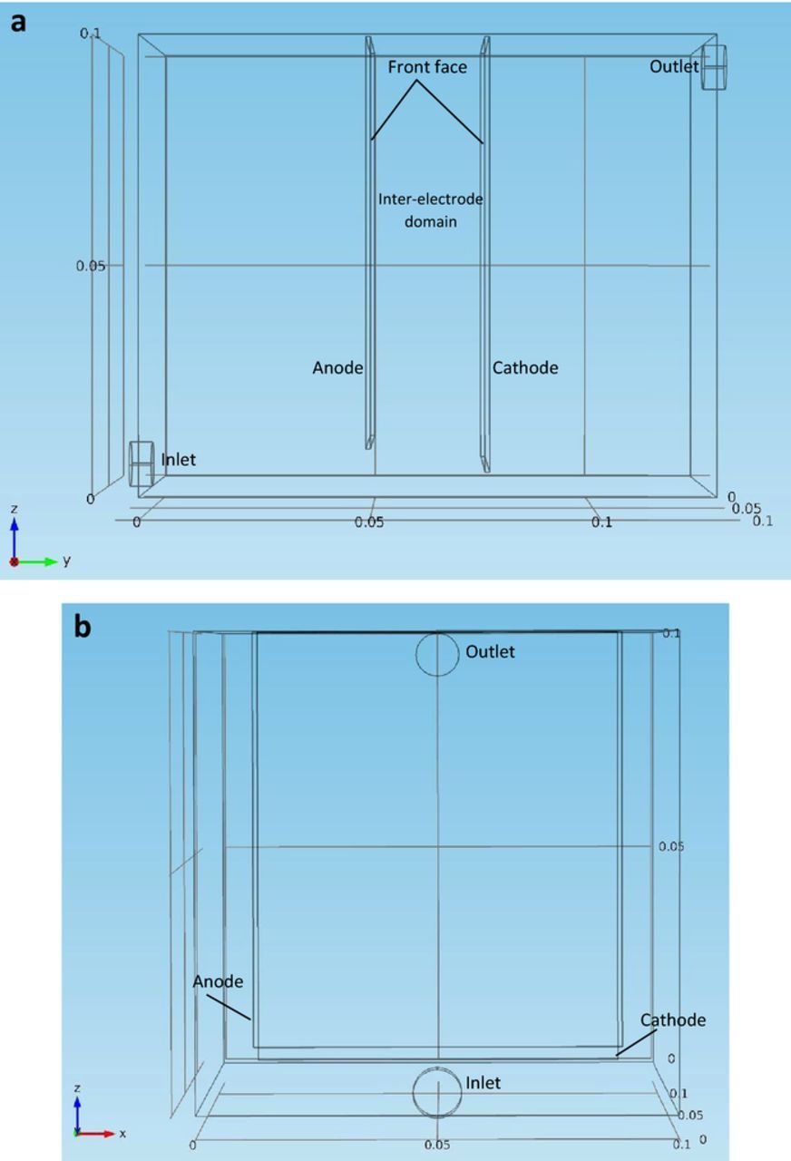
Figure 1. (a) – 1(b) Geometry of the three dimensional copper electrorefining cell used for the model from different angles: front view (a) and side view (b).
Mesh
Through the development of the multi-phase flow copper electrorefining model, meshes in this electrolytic cell have been refined especially for boundary layer meshes. The simulation results using the current meshes show no appreciable difference from those using the last coarser meshes. The domain of this three dimensional electrorefining cell were discretized into tetrahedral mesh elements (0.0053 m of the maximum element size and 0.001 m of the minimum element size) as shown in Figure 2a. The geometric faces in the cell were discretized into triangular elements (0.0023 m of the maximum element size and 0.00015 m of the minimum element size). Layers of finer elements are over all faces. There are four boundary layers over the anode and cathode faces as shown in Figure 2b. The layer thickness is 0.0001 m for the first boundary layer and increases by 20% after then. Other faces have two boundary layers, with the thicknesses of the first and second layers to be 0.00129 m and 0.00155 m, respectively. The geometric edges and vertices were discretized into edge elements and vertex elements.
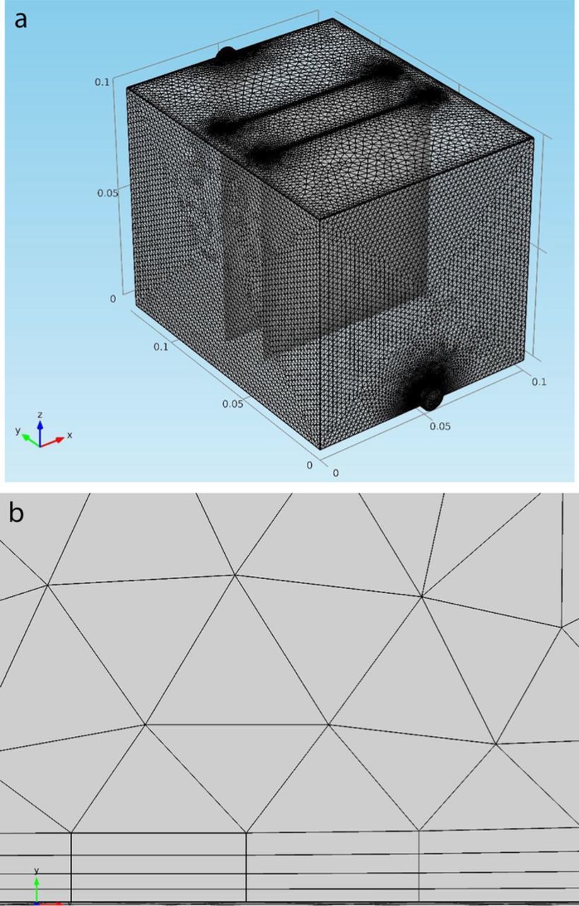
Figure 2. (a) – 2(b) Meshes of the three dimensional copper electrorefining cell used for the model (a) and boundary layer meshes over the anode face (b).
Time-dependent simulation numerical procedure
The time-stepping algorithms used in the time-dependent simulation in this study is the backward differentiation formula (BDF), which involves two tolerances: the relative tolerance (Rtol) and the absolute tolerance (Atol). The relative tolerance is employed in every iteration for all dependent variables and is a dimensionless quantity, while the absolute tolerance is also employed in every iteration but has units depending on the dependent variable to which it applies. The time-dependent solver can go to the next time step if the estimated local error vector  in the integration step meets the following inequality:18
![Equation ([28])](https://content.cld.iop.org/journals/1945-7111/164/9/E233/revision1/d0028.gif)
where  is the vector of dependent variables, Rtol is the dimensionless relative tolerance that is set at 1.0E-3 in the simulation,
  is the absolute tolerance for dependent variable
  and has a global value of 5.0E-4.
For the BDF time-stepping method, the initial time step is set at 0.001 s; the maximum time step is 0.1 s; the maximum and minimum BDF orders are 2 and 1, respectively. In each time step, dependent variables are segregated into three groups that are solved by three steps. The first segregated step solves for dependent variables in the current distribution model including species concentrations and current densities; the second segregated step solves for mixture velocity field and pressure; the third segregated step solves for the volume fraction of dispersed phase and the squared slip velocity.
Results and Discussion
Copper electrorefining involving slime particle transport was simulated in the three dimensional cell described in section Geometry, using the two-phase flow model and current distribution model described in sections The two-phase flow model and The current distribution model. Two different slime particle releasing scenarios were simulated: (1) impurity particles are released only from the inlet; (2) impurity particles are released from both the inlet and the anode front face. Dispersed phase volume fractions on the inlet face and the anode front face are specified in Table I. In both cases, the initial dispersed phase volume fraction in the electrorefining cell was defined as one tenth of the inlet dispersed phase volume fraction. One hour of simulation was performed for both scenarios.
Impurity particles released from the inlet only
The fluid flow field in a copper electrorefining cell is usually driven by electrolyte inflows, as well as electrolyte density gradients that are formed mainly due to cupric ion accumulation near anodes and depletion near cathodes. Besides, cupric ion plays a vital role in carrying electrolyte current densities. Furthermore, cupric ion depletion near cathodes is the main barrier of applying high current densities. As a result, cupric ion distribution in an electrorefining cell is of great significance. Figures 3a–3c present cupric ion concentration profiles and electrolyte current density distributions at different time points in the electrolytic cell defined in section Geometry.
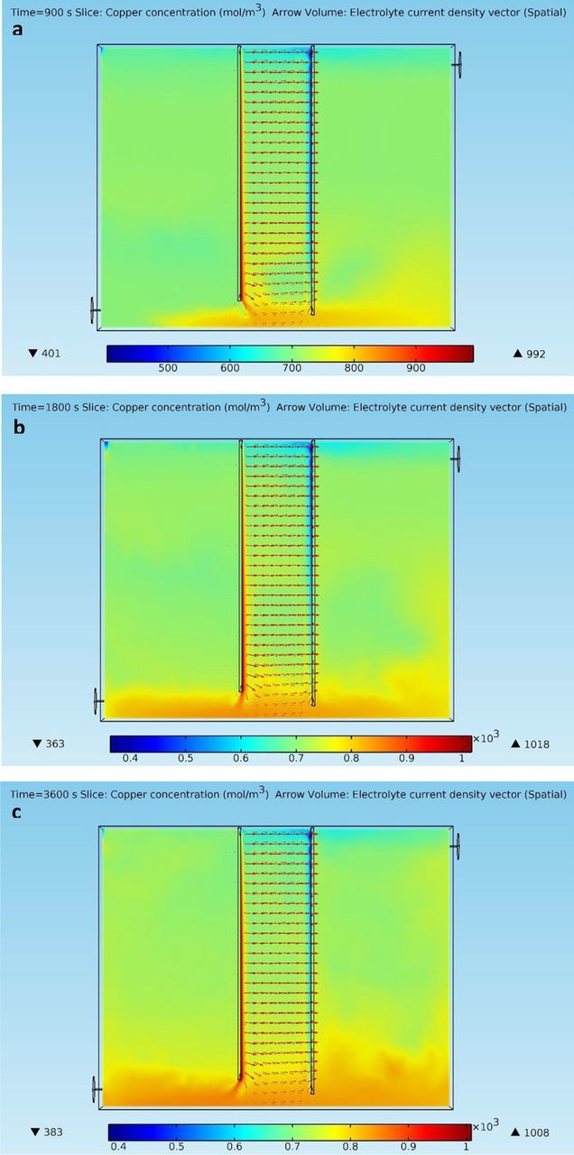
Figure 3. (a) – 3(c) Cupric ion concentration profiles and electrolyte current density distributions at different time points in the copper electrorefining cell defined in section Geometry with dispersed phase particles released from the inlet (color represents cupric ion concentration in mol/m3, and arrows are electrolyte current density vectors).
As shown in Figures 3a–3c, cupric ion distribution in the cell varies as time goes, especially at the bottom of the cell. Copper accumulation zone (red stripe) and depletion zone (blue stripe) are formed as early as t = 900 s, along the anode and the cathode, respectively. Most areas in the cell have copper concentrations near the initial concentration of 708 mol/m3. However, more and more cupric ions are transported to the bottom domain of the cell, due to the downward fluid flows at the anode bottom. The affected area may further expand from the cell bottom at even later time points, but the bulk copper concentrations in most areas would not be raised significantly. Because most cupric ions produced from the anode are eventually transferred to the cathode surface under the combined effects of convection, migration, and diffusion, although they are apparently deviated from direct paths to the cathode by the strong downward flows. As seen in Figures 3a–3c, cupric ion concentrations near the cathode bottom are larger than those near the cathode top, due to the replenishment of cupric ions from the anode and consumption of cupric ions at the cathode. Electrolyte current densities at the electrode bottom are also affected by the deviated transfer of cupric ions, as current from the anode bottom edge is curved toward the cell bottom before it turns back to the cathode. Electrolyte current densities at higher positions are perpendicular to the parallel electrodes. In addition, curved blue stripe at the cell top also reflects the effects of fluid flows, which are in the shape of loops within the inter-electrode domain, as shown in Figures 4a–4d. These copper-deficient electrolytes are then gradually replenished with cupric ions as they flow down along the anode.
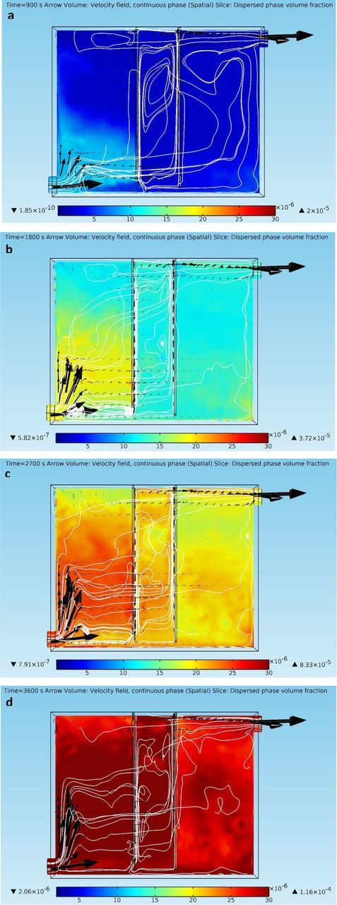
Figure 4. (a) – 4(d) Continuous phase velocity fields and dispersed phase (impurity particles) volume fraction profiles at different time points in the copper electrorefining cell defined in section Geometry with dispersed phase particles released from the inlet (arrows represent liquid phase velocity vectors, white lines are liquid phase velocity field streamlines, and color presents volume fractions of the dispersed phase).
Figures 4a–4d show the behaviors of the liquid phase and the impurity particle phase in copper electrorefining as time goes. The continuous phase (electrolyte) is tracked through its velocity field, whereas the dispersed phase is tracked through its volume fraction. As shown in Figures 4a–4d, the velocity field of the liquid phase is driven by the inflow electrolyte momentum and the electrolyte density gradients between the electrodes. At t = 900 s, the looping flows have been already formed within the inter-electrode gap, with upward flows along the cathode and downward flows along the anode. Some of the downward fluid flows from the anode bottom go to the right side of the cell and turn up when approaching the cell right wall. The electrolyte inflows have limited influence on the fluid flow field between the electrodes, due to the dominance of the density gradient driven looping flows in this domain. At the bottom of the electrodes, strong downward flows from the anode act like barriers for the electrolyte inflows to go through. As a result, most of the electrolyte inflows turn up, cross over the inter-electrode domain at higher positions where there are gaps between cell side walls and electrode side edges (shown in Figures 5a–5c), and exist the electrorefining cell through the upper outlet. Nevertheless, some of these flows enter the inter-electrode domain and merge with the looping flows there, instead of crossing over the domain. This results in the transport of dispersed phase particles into the inter-electrode domain, as discussed next. In general, species transfer within the inter-electrode domain mostly relies on natural convection (looping fluid flows), whereas species transport outside the inter-electrode domain depends on forced convection (electrolyte inflows).
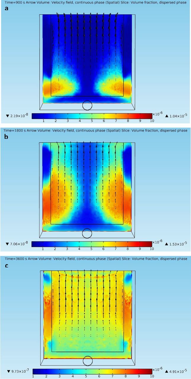
Figure 5. (a) – 5(c) Continuous phase velocity fields and dispersed phase (impurity particles) volume fraction profiles on a slice 100 microns away from the cathode front face at different time points in the copper electrorefining cell defined in section Geometry with dispersed phase particles released from the inlet (arrows are liquid phase velocity vectors, and color represents volume fractions of the dispersed phase).
The dispersed phase of impurity particles enters the cell through the inlet continuously with the same initial velocity as the liquid phase. As shown in Figures 4a–4d, some of the dispersed phase particles settle down and form a layer with high volume fractions of the dispersed phase on the cell bottom, which becomes thicker and denser as time goes. Most of the dispersed phase particles, however, are carried upward and forward by the flowing liquid phase. Impurity particles that reach the edges of the anode are approaching the inter-electrode domain. Part of them can pass through the domain through the side gaps between cell walls and electrode edges, and enter the right side of cell, forming irregular shaped mixture rich in dispersed phase under the effects of local fluid flows. Nevertheless, most of these impurity particles that approach the inter-electrode gap are further transported into the gap and are taken over by the looping fluid flows. This is shown clearer at a different angle in Figures 5a–5c. Within the inter-electrode gap, the dispersed phase particles climb up along the cathode, settle down along the anode, and lead to high dispersed phase volume fraction mixture near the electrodes, as a result of the interaction between drag forces and gravity. As more and more impurity particles enter the inter-electrode domain, the stripes expand and fill up most of the domain with larger and larger volume fractions of the dispersed phase. Some dispersed phase particles within the gap can be carried by the downward flows from the anode bottom and travel to the right side of the cell or settle down into the rich dispersed phase layer on the cell bottom. On the left side of the electrorefining cell, the solid dispersed phase expands and accumulates continuously as more impurity particles enter the cell and are carried up by the upward flowing liquid phase.
Since impurity particles are the major source of cathode contamination in copper electrorefining,3 the distribution of the solid dispersed phase within a short distance from the cathode front face becomes significant. Figures 5a–5c present the electrolyte velocity fields and the dispersed phase volume fraction distributions in front of the cathode at different time points. Notice that the smaller rectangle inside the cell is the cathode front face, and there are two narrow gaps between the cathode side edges and the cell side walls.
As shown in Figures 5a–5c, it is clear that most liquid phase velocity vectors are almost parallel to the vertical direction, indicating that upward vertical fluid flows are dominant in front of the cathode. The magnitudes of the upward fluid flows increase gradually from the cathode bottom to its top due to the effects of fluid density gradients. In front of the side fringes of the cathode, the liquid phase velocity vectors are slightly tilted toward the center, which results from the interaction of the incoming outside flows and the inside looping flows. As discussed, the dispersed phase of impurity particles can enter the inter-electrode domain from the side gaps. It is clearly shown in Figures 5a–5c that mixtures with large volume fractions of the dispersed phase begin to enter the domain at t = 900 s. As time goes, the mixtures spread out in the domain and appear in front of the whole cathode front face. However, most impurity particles are more likely to contaminate the side parts of the cathode rather than its center part, as the side parts continuously show larger volume fractions of the dispersed phase than the center part. According to the impurity data of the cathodes harvested in a similarly shaped electrorefining cell with impurity particles released from its inlet in previous research,6 the side part of the harvested cathodes contain 7.75 wt% of impurity particles in average, and the center part only have 2.93 wt% of impurity particles in average. Therefore, the experimental results show some similar phenomena as presented in the simulation. This phenomenon is mostly likely because impurity particles enter the inter-electrode domain from its sides rather than its bottom, where the downward fluid flows from the anode prevent electrolyte inflows or impurity particles from entering. As a result, the side parts of the cathode would be continuously exposed to larger volume fractions of the solid dispersed phase, a major cathodic contamination source, than the center part of the cathode.
Impurity particles released from both the inlet and the anode
The cupric ion concentration profiles and electrolyte current density distributions in this scenario are similar to those in the previous scenario, and thus will not be discussed. In this scenario, dispersed phase particles are also released from the anode front surface, with a dispersed phase volume fraction about five times larger than that on the inlet face. Thus, the cathode surface may encounter more impurity particles. The resulting solid dispersed phase distributions and liquid phase velocity fields at different time points are shown in Figures 6a–6d. The time points chosen here are 180 s, 900 s, 1800 s, and 3600 s, in order to show dispersed phase distributions at earlier time points. Note that Figures 6c–6d have different color scales from those in Figures 6a–6b, due to much larger dispersed phase volume fractions to express.
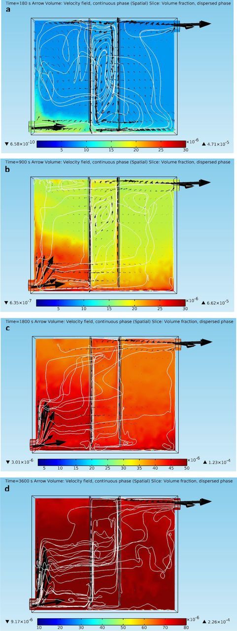
Figure 6. (a) – 6(d) Continuous phase velocity fields and dispersed phase (impurity particles) volume fraction profiles at different time points in the copper electrorefining cell defined in section Geometry with dispersed phase particles released from both the inlet and the anode front face (arrows represent liquid phase velocity vectors, white lines are liquid phase velocity field streamlines, and color presents volume fractions of the dispersed phase).
At t = 180 s, dispersed phase particles that released from the anode front face drop down with the downward fluid flows along the anode and settle on the cell bottom, with those released from the inlet approaching the bottom of the inter-electrode gap. At t = 900 s, mixtures containing large volume fractions of the solid dispersed phase already appear in front of the cathode, as a result of the transport of impurity particles from the anode. Notice that dispersed phase with significant volume fractions does not show up in front of the cathode at t = 900 s and 1800 s in the previous scenario. Besides, the layer of high dispersed phase volume fractions on the cell bottom is much thicker under this scenario, due to the settlement of dispersed phase particles from the anode. At t = 1800 s and 3600 s, this layer merges with the mixture rich in dispersed phase in the inter-electrode gap. As shown in Figures 6a–6d, the dispersed phase fills up the electrorefining cell, especially the inter-electrode domain, at a much faster speed than the previous scenario. The current scenario shows much larger dispersed phase volume fractions all over the copper electrorefining cell at the same time points. Obviously, this is due to the dispersion of the impurity particles released from the anode front face. In addition, the electrolyte velocity field in this scenario shows some variations from that in the previous scenario, as denser mixtures flow down and spread out from the anode bottom, and exert effects on the fluid flow fields at other parts of the cell. The distribution of dispersed phase particles in front of the cathode may vary under this scenario and should be further discussed. Figures 7a–7c present the electrolyte velocity fields and the solid dispersed phase distributions in front of the cathode at different time points under the current scenario. Note that Figure 7c has different color scales than those in Figures 7a–7b.
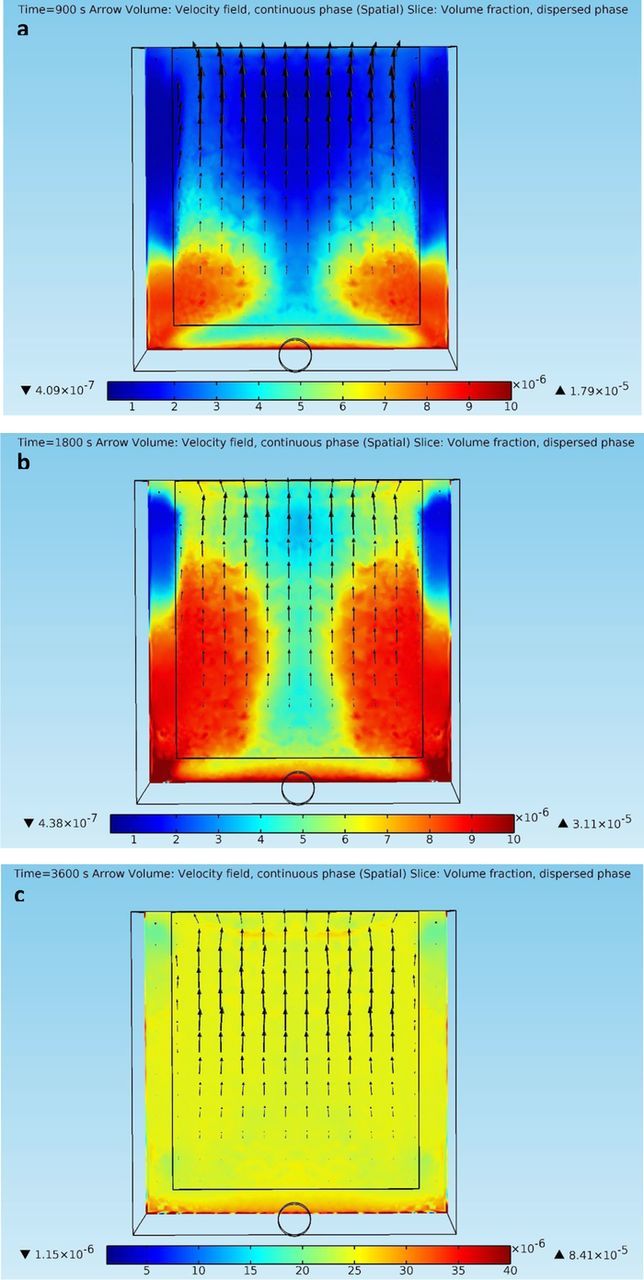
Figure 7. (a) – 7(c) Continuous phase velocity fields and dispersed phase (impurity particles) volume fraction profiles on a slice 100 microns away from the cathode front face at different time points in the copper electrorefining cell defined in Geometry section with dispersed phase particles released from both the inlet and the anode front face (arrows are liquid phase velocity vectors, and color represents volume fractions of the dispersed phase).
As shown in Figures 7a–7c, the dispersed phase distributions on the slice 100 microns away from the cathode front face show similar features as those in the previous scenario. However, some appreciable differences can be found. It seems that dispersed phase particles from the inlet still play a main role in the particles approaching the cathode, as they enter the inter-electrode gap from both sides. Nevertheless, impurity particles released from the anode front face are also transported to the area in front of the cathode as they can be picked up by looping electrolyte flows. As shown in Figures 7a–7b, the green and yellow areas above the layer rich in dispersed phase on the cell bottom represent the impurity particles that are picked by the looping flows. Whereas in Figures 5a–5b, these areas are blue, indicating very few dispersed phase particles. The dispersed phase volume fractions in the mixtures entering from the sides also become larger due to the participation of picked up impurity particles, if compared with those in the previous scenario. At t = 3600 s, the dispersed phase distribution becomes almost uniform in front of the cathode, as the result of the involvement of anode impurity particles. Nevertheless, as shown in Figures 7a–7b, a significant amount of dispersed phase particles from the anode settle down to the red layer on the cell bottom, which gradually becomes thicker and denser, with fewer impurity particles picked up by looping flows. To sum up, when impurity particles are released from both the inlet and the anode, the side parts of the cathode front face encounter more dispersed phase particles at initial stages, but have almost the same amount of approaching impurity particles as the center part of the cathode at later stages.
Conclusions
In order to simulate fluid flow and impurity particle simultaneously in copper electrorefining, a two-phase flow model was developed, with electrolyte as a liquid phase and impurity particles as a dispersed phase. Copper electrorefining in a lab-scale three dimensional cell was simulated for two different impurity particle releasing scenarios using the model. The results of cupric ion distributions, electrolyte current density distributions, electrolyte flow fields, and solid dispersed phase distributions were discussed.
The first scenario simulated has impurity particles released only from the inlet face. The resulting cupric ion distributions show copper accumulation and depletion zones near the electrodes. More importantly, a significant amount of cupric ions are transported to the cell bottom due to the downward electrolyte flows at the anode bottom. However, bulk copper concentrations in most areas are not severely affected. Electrolyte current density distributions are also influenced by the deviated transfer of cupric ions, as current density vectors from the anode bottom are curved toward the cell bottom. The fluid flow field results show that looping flows are dominant in the inter-electrode gap and even have effects on the fluid flow fields on other parts of the cell. The electrolyte inflows prefer to enter or flow over the inter-electrode domain through the side gaps between the electrode edges and cell walls, rather than the bottom of the electrodes. According to the dispersed phase distribution results, dispersed phase particles are transported to the inter-electrode domain by the electrolyte inflows through the side gaps. However, a large number of impurity particles settle to the cell bottom after released from the inlet. Dispersed phase particles move in the inter-electrode gap under the combined effects of drag forces and gravity. Impurity particles are accumulated in the inter-electrode gap as time goes, with some of them settling down or traveling to the right side of the cell. From the dispersed phase distributions in front of the cathode, the side parts of the cathode encounter more dispersed phase particles and are more likely to be contaminated than the center part of the cathode, as impurity particles enter the inter-electrode domain from the side gaps. Experimental results demonstrate similar phenomena.
The second scenario simulated has dispersed phase particles released from both the inlet and the anode front face. The copper electrorefining cell is filled up with the dispersed phase with a much faster rate, and the cathode front face encounters mixtures with significant volume fractions of dispersed phase much earlier. The rich dispersed phase layer on the cell bottom is also much thicker in this scenario. The electrolyte velocity field shows some variations due to the effects of denser mixture flows from the anode. The dispersed phase distributions in front of the cathode in this scenario show that impurity particles from the inlet still have strong influence on the distributions, but dispersed phase particles from the anode are also transported to the cathode although a significant amount of them settle to the cell bottom. In this scenario, the side parts of the cathode are exposed to more impurity particles than the center part only at initial stages. At later stages, dispersed phase particles are distributed almost uniformly in front of the cathode.
List of Symbols
| ci | concentration of species i, mol/m3 |
| [Cu] | local cupric ion concentration, mol/m3 |
| CCu | cupric ion concentration at the interface, mol/m3 |
 |
bulk or initial cupric ion concentration, mol/m3 |
| CH2SO4 | initial H2SO4 concentration, kg/m3 |
| dd | dispersed phase particle diameter, m |
| Di | diffusivity of species i, m2/s |
| F | Faraday's constant, 96485 C/mol |
 |
volume force, N/m3 |
| iaverage | average current density on the anode, A/m2 |
| iloc | local current density at the electrode-electrolyte interface, A/m2 |
| i0 | equilibrium exchange current density, A/m2 |
 |
electrolyte current density, A/m2 |
 |
mass transfer rate from dispersed phase to continuous phase, kg · m−2 · s−1 |
 |
unit normal vector to surface |
 |
flux density of species i, mol · m−2 · s−1 |
| p | pressure, Pa |
| T | absolute temperature, K |
| ui | mobility of species i, m2 · V−1· s−1 |
 |
mixture velocity, m/s |
 |
velocity of the continuous phase, m/s |
 |
velocity of the dispersed phase, m/s |
 |
slip velocity between the continuous phase and the dispersed phase, m/s |
| wd | dispersed phase mass fraction |
| zi | charge number of species i |
Greek
| αa, αc | anodic and cathodic symmetry factors |
| η | local overpotential at the interface, V |
| μ | mixture dynamic viscosity, kg · m−1 · s−1 |
| μc | continuous phase dynamic viscosity, kg · m−1 · s−1 |
| ρ | mixture density, kg/m3 |
| ρc | continuous phase density, kg/m3 |
| ρd | dispersed phase particle density, kg/m3 |
| ϕc | continuous phase volume fraction |
| ϕd | dispersed phase volume fraction |
| ϕmax | the maximum packing volume fraction |
| Φl | electrolyte potential, V |
| ΦS | electrode potential, V |
| ΔΦeq | equilibrium potential difference, V |