Abstract
A model based in COMSOL Multiphysics consisting of an electrorefining cell was utilized to simulate copper electrorefining. Concentration and electrolyte density profiles were generated as electrochemical simulation results. Fluid velocity field, particle trajectories, and particle distribution maps were generated to study impurity particle behavior in electrolyte. A three factor designed set of boundary conditions was used to determine the effects of inlet flow rate, temperature, and current density on impurity particle behavior in electrolyte and the associated distribution on the cross section (slice) 100 microns away from the front surface of the cathode during copper electrorefining. The number of impurity particles on the cross section was counted for each set of boundary conditions. The model data for impurity particle distribution was compared with measured impurity particle contamination at the cathode surface, and the results show a very good correlation, which suggests the model is reasonable. The model results show the three factors have significant effects on the number of impurity particles on the cross section. The impurity particle counts at the corner positions of the slice are much higher than those at the center position of the slice. Possible explanations for the simulation results are proposed.
Export citation and abstract BibTeX RIS

This is an open access article distributed under the terms of the Creative Commons Attribution 4.0 License (CC BY, http://creativecommons.org/licenses/by/4.0/), which permits unrestricted reuse of the work in any medium, provided the original work is properly cited.
Cast anode has inclusions within the copper matrix, due to the existence of its inherent impurities such as lead, arsenic, bismuth, antimony, and silver impurities. During electrorefining, copper in the anode dissolves. As a result, many of these inclusions are liberated in the electrolytic solution as anode slimes, though some of them stick to the remaining anode by adhesion. Anode slimes that are larger and denser tend to settle to the bottom of the cells. Nevertheless, finer anode slimes do not settle, but remain in suspension in solution. They can be transported and incorporated into cathodes.1–3 Consequently, anode slimes are a major potential source of impurities in the cathode.4–7
To improve cathode purity, anode slime transport in the flowing electrolyte has been studied. There are some studies on modelling and measurement of flow in electrorefining cells, which indicate the existence of recirculation between anodes and cathodes.8–10 Many studies considering anode slime and its characteristics have been performed.11–13 But flow studies involving slimes are rarely found in the literature, and the major electrorefining parameters' effects on slime behavior in electrolytic solution are not well known.
Modeling and simulations can be cost effective ways of predicting the behavior of impurity particles in the electrolytic solution. Models can compute the solution concentrations, electrolyte density distribution, fluid velocity, particle trajectories, and particle distributions.
There are several commercially available software packages on the market, including Elsyca, Cell Design, and COMSOL Multiphysics.14 These software packages make complex geometries modeling and complex simulations, such as particle tracing, possible.15
In this study, modeling, simulation, and experimental validation of the copper electrorefining process was completed to understand the behavior of anode slimes in flowing electrolyte and their distribution on the cross section 100 microns away from the front surface of the cathode. COMSOL Multiphysics with its Electrodepostion, Computational Fluid Dynamics, and Particle Tracing modules, was utilized to simulate the process.
COMSOL Multiphysics is capable of combining electrodeposition, fluid flow, and particle tracing into one model. Furthermore, it has the ability to model in three dimensions and provide results in three dimensional images and animations.16 COMSOL Multiphysics uses the finite element method to compute model solutions.
Model Description
Governing equations description
To model the electrodeposition process in the study, the Tertiary Nernst-Planck interface was utilized to solve for the electrolyte potential (Φl), the current density distribution ( ), and the concentrations of various species (ci).15 A set of governing equations was used and solved.17,18
In electrolyte, the governing equation for the mass transfer in the solution is the Nernst-Plank equation:
![Equation ([1])](https://content.cld.iop.org/journals/1945-7111/162/14/E338/revision1/d0001.gif)
where  , zi, ui, ci, Di are the flux density, charge, mobility, concentration, and diffusivity of species i, F is Faraday's constant, − ∇Φl is an electric field, ∇ci is a concentration gradient, and
  is the velocity vector.
No homogeneous reaction in the electrolyte in the electrorefining cell was assumed, so material balance is governed by the equation:
![Equation ([2])](https://content.cld.iop.org/journals/1945-7111/162/14/E338/revision1/d0002.gif)
In the electrolyte, the current density is governed by:
![Equation ([3])](https://content.cld.iop.org/journals/1945-7111/162/14/E338/revision1/d0003.gif)
where  is the current density in the electrolyte, and other variables are defined previously.
Due to the electroneutrality of the electrolytic solution, the last term on the right is zero (∑zici = 0). Therefore,
![Equation ([4])](https://content.cld.iop.org/journals/1945-7111/162/14/E338/revision1/d0004.gif)
On the electrodes, the current density is governed by Ohm's Law:
![Equation ([5])](https://content.cld.iop.org/journals/1945-7111/162/14/E338/revision1/d0005.gif)
where is is the current density in the electrode, σs is the conductivity of the electrode and ∇Φs is an electric field. It was assumed that the electric potential on the anode and cathode was constant, due to their much lower electric resistance compared to the electrolyte. Note that only the front side face of each electrode had electrode reactions with all other faces insulated (see Model geometry section and associated figures). The electric potential of the cathode (the front side face) was assumed to be 0 V and therefore all other potentials were measured with this reference.
With conservation of current in the electrolyte and electrodes, we have:
![Equation ([6])](https://content.cld.iop.org/journals/1945-7111/162/14/E338/revision1/d0006.gif)
where k denotes an index that is l for the electrolyte and s for the electrode, and Qk is a general current source term and was zero in this model.18 Therefore, Eq. 6 becomes:
![Equation ([7])](https://content.cld.iop.org/journals/1945-7111/162/14/E338/revision1/d0007.gif)
At the electrode-electrolyte-interface, the overpotential η (the driving force for the electrochemical reactions at the interface) is defined as:
![Equation ([8])](https://content.cld.iop.org/journals/1945-7111/162/14/E338/revision1/d0008.gif)
where ΦS is the electric potential of the electrode, Φl is the potential of the electrolyte adjacent to the electrode, and ΔΦeq is the difference between the electrode and the electrolyte potentials at the interface measured at equilibrium using a common reference potential18 and was assumed to be zero in this model. Since the electric potential of the electrode was assumed to be constant, it was the electrolyte potential at the interface that would lead to the variations in the overpotential.
The local overpotential determines the local current density at the electrode-electrolyte-interface by the concentration dependent Butler-Volmer equation:
![Equation ([9])](https://content.cld.iop.org/journals/1945-7111/162/14/E338/revision1/d0009.gif)
where iloc is the local current density at the interface (also called as charge transfer current density), i0 is equilibrium exchange current density, CR, S is the surface reductant concentration, CR, B is the bulk reductant concentration, CO, S is the surface oxidant concentration, CO, B is the bulk oxidant concentration, αa is the anodic symmetry factor, αc is the cathodic symmetry factor, z is the number of electrons transferred in the rate limiting step (typically 1), F is the Faraday constant, R is the gas constant, T is the absolute temperature, and η is the overpotential.1,18 The values of equilibrium exchange current density, anodic and cathodic symmetry factors, and the temperature are specified in Table II (the equilibrium exchange current density and anodic and cathodic symmetry factors were assumed to be the typical values in copper electrorefining),19 and they are the same for both anodic and cathodic reactions. The value of  is 1 for both anodic and cathodic reactions, since the reduced species in both reactions is copper in solid state. The expression for
  is
is  , where CCu is the localized time-dependent concentration of cupric ions at the interface and
  is the initial cupric ion concentration in the cell that is equal to the bulk cupric ion concentration.
Table II. Main parameters set in the model.
| Description | Value | Description | Value |
|---|---|---|---|
| Exchange current density | 0.2 [A/m2] | Anode symmetry factor | 1.5 |
| Temperature | 323.15/343.15 [K] | Cathode symmetry factor | 0.5 |
| Concentration of H2SO4 | 180 [g/l] | Initial concentration of cupric ion | 45 [g/l] |
| (Average) Current density | 225/375 [A/m2] | Inlet flow rate | 3.5/11 [ml/min] |
| Impurity particle diameter | 14.5E-6 [m] | Impurity particle density | 4200 [kg/m3] |
Besides the conservation of current in the electrolyte and electrodes, the current must also be conserved at the electrode-electrolyte-interface. In this model, current is transferred between the electrolyte and electrode domains by an electrochemical reaction (Faradaic current). Thus the current density in the electrolyte adjacent to the electrode has the following relationship with the local current density term in the Butler-Volmer equation:18
![Equation ([10])](https://content.cld.iop.org/journals/1945-7111/162/14/E338/revision1/d0010.gif)
where  is the current density in the electrolyte at the interface,
  is the unit normal vector to the electrode surface, and iloc is the local current density.
This current density distribution model had the average current density on the anode, rather than the electric potentials of the electrodes, as the boundary condition. Besides, the balance of current (an equal amount of current that left at the anode also enters at the cathode) needs to be satisfied. Therefore, the current densities in the electrolyte adjacent to the electrode are constrained by the following integral equations:
![Equation ([11])](https://content.cld.iop.org/journals/1945-7111/162/14/E338/revision1/d0011.gif)
where  is the current density in the electrolyte adjacent to the electrode,
 is the unit normal vector to the electrode surface, and iaverage is the average current density applied.18
In this model, the electrolyte current density  , the electrolyte potential Φl are governed by Eq. 4 and Eq. 7 in the electrolyte and by Eqs. 8–11 at the interface, while the electrode potential Φs and current density is are governed by Eq. 5 and Eq. 7 on the electrodes and by Eqs. 8, 9 at the interface. The Butler-Volmer equation connects the electrode and electrolyte variables at the interface through overpotential η and local current density iloc. Note that the electrode potential and current density are peripheral to this model and the electrodes are just two geometric faces in the model as discussed previously. The species concentration ci can be solved with the addition of Eq. 2. The flow velocity term
  in Eq. 1 connects the current distribution with flow field. As a result, with the constraint of Eq. 1 to Eq. 11, the electrolyte potential, the current density distribution, and concentrations of various species can be solved, given the parameters (such as diffusivity Di and mobility ui) and boundary conditions (such as average current density iaverage).
The laminar flow interface was chosen to model the fluid flow in this study and it was coupled with the current distribution model. Turbulence was not considered here because of the small dimensions of both inlet pipe and the electrochemical cell, and the low flow rates exerted and internally generated. Thus the Reynolds numbers of the flow in the pipe (about 32.86 at the flow rate of 11 ml/min) and in the cell (about 141 in the inter-electrode domain using the highest flow velocity of the flow between the electrodes) are relatively low. The flow field and current distribution could almost reach steady state after 5000 s in the time-dependent simulation and the steady state solutions were also obtained by further stationary simulation, which are shown in Simulation results and discussion section. Furthermore, it was assumed that the impact of impurity particles on the fluid velocity field is negligible. Lastly, the general particle trajectory caused by the general fluid field driven by the inlet inflow and the density gradients between the electrodes is the main issue studied in this paper and the minor turbulence in the cell and the turbulent dispersion of particles is not considered in this study but could be considered for future work. Another set of governing equations was used and solved for fluid flow.18,20
A variable density flow was assumed, dependent on temperature and concentrations of cupric ions and acid. It is governed by the following continuity and momentum equations:
![Equation ([12])](https://content.cld.iop.org/journals/1945-7111/162/14/E338/revision1/d0012.gif)
![Equation ([13])](https://content.cld.iop.org/journals/1945-7111/162/14/E338/revision1/d0013.gif)
where ρ is the density, v is the fluid velocity vector, p is the pressure, μ is the dynamic viscosity, I is the identity tensor, and F is the body force vector (per unit volume) acting on the fluid.
Simulations of the impurity particle motion in the electrolytic solution were time dependent and were based on fluid flow field solutions. Negligible impact of particles on the flow velocity field was assumed. The motion of a particle is governed by Newton's second law:
![Equation ([14])](https://content.cld.iop.org/journals/1945-7111/162/14/E338/revision1/d0014.gif)
where m is the particle mass, x is the position of the particle, and F is the sum of all forces acting on the particle, such as drag and gravity forces.18
Model geometry
The geometry of the model is presented in Figures 1a–1b with a three dimensional coordinate system. The size of the cell is 0.125 × 0.10 × 0.10 m. The anode is 0.08 × 0.09 × 0.001 m in size, and the cathode is 0.08 × 0.095 × 0.001 m in size. The distance between the anode and the cathode is 0.025 m. The inflow pipe is 0.005 m in radius and 0.002 m in length. The axis of the inflow pipe is in the y direction, with its coordinates of x = 0.05 m and z = 0.005 m. The outflow pipe is also 0.005 m in radius and 0.002 m in length. The axis of the outflow pipe is in the y direction, with its coordinates of x = 0.05 m and z = 0.095 m.

Figure 1. (a) The geometry of the copper electrorefining cell in the COMSOL model (all units in meters). (b) The geometry of the copper electrorefining cell in the COMSOL model (all units in meters).
As shown in Figures 1a–1b, only the front side faces of the anode and the cathode were selected to have electrode reactions. The left end of the inflow pipe was selected as the inlet, while the right end of the outflow pipe was selected as the outlet.
Model boundary conditions
The anodic reaction and cathodic reactions were assumed to be:
![Equation ([15])](https://content.cld.iop.org/journals/1945-7111/162/14/E338/revision1/d0015.gif)
![Equation ([16])](https://content.cld.iop.org/journals/1945-7111/162/14/E338/revision1/d0016.gif)
Faces other than the two electrode faces, were set to have insulation boundary condition:
![Equation ([17])](https://content.cld.iop.org/journals/1945-7111/162/14/E338/revision1/d0017.gif)
where  is the unit normal vector to the face, and i is the current density.
Faces other than the two electrode faces, the inlet face, and the outlet face, were set to have no flux boundary condition:
![Equation ([18])](https://content.cld.iop.org/journals/1945-7111/162/14/E338/revision1/d0018.gif)
where  is the unit normal vector to the face, and
  is the flux density of species i.
The conductivity of the solution is governed by the following equation:17
![Equation ([19])](https://content.cld.iop.org/journals/1945-7111/162/14/E338/revision1/d0019.gif)
where σ is the conductivity of the solution, F is Faraday's constant, and zi, ui, ci are the charge, mobility, and ccentration of species i.
The diffusivity was estimated using the equation:
![Equation ([20])](https://content.cld.iop.org/journals/1945-7111/162/14/E338/revision1/d0020.gif)
where D is the diffusivity, D0 is the maximum diffusivity at infinite temperature, R is the gas constant, T is the absolute temperature, and Ea is the activation energy for diffusion.
The following empirical equation was derived from the experimental data from Moats et al.:21
![Equation ([21])](https://content.cld.iop.org/journals/1945-7111/162/14/E338/revision1/d0021.gif)
where D is the diffusivity in cm2/s, CH2SO4 is the initial H2SO4 concentration in Kg/m3, [Cu] is the localized cupric ion concentration in mol/m3, and T is the absolute temperature in Kelvin. The fitting plot for the diffusivity is shown in Figure 2.
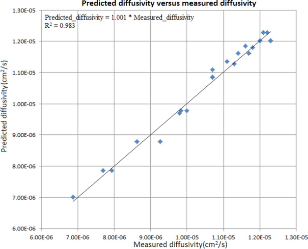
Figure 2. Fitting plot of predicted diffusivity versus measured diffusivity.
The diffusivity in this study was treated as an overall diffusivity. For every set of cell conditions, cupric ions, sulfate ions, and hydrogen ions were assumed to have the same overall diffusivity.
The mobility was calculated using the relationship:
![Equation ([22])](https://content.cld.iop.org/journals/1945-7111/162/14/E338/revision1/d0022.gif)
where ui and Di are the mobility and diffusivity of species i, R is the gas constant, and T is the absolute temperature.
The electrolyte density in the cell was estimated by the following equation, modified from the empirical equation tt Price and Davenport derived from their experimental data:22
![Equation ([23])](https://content.cld.iop.org/journals/1945-7111/162/14/E338/revision1/d0023.gif)
where ρ is the fluid density in kg/m3, [Cu] is the localized cupric ion concentration in mol/m3, CH2SO4 is the initial H2SO4 concentration in Kg/m3, and T is the temperature in degree C. The fitting plot for the electrolyte density is shown in Figure 3.
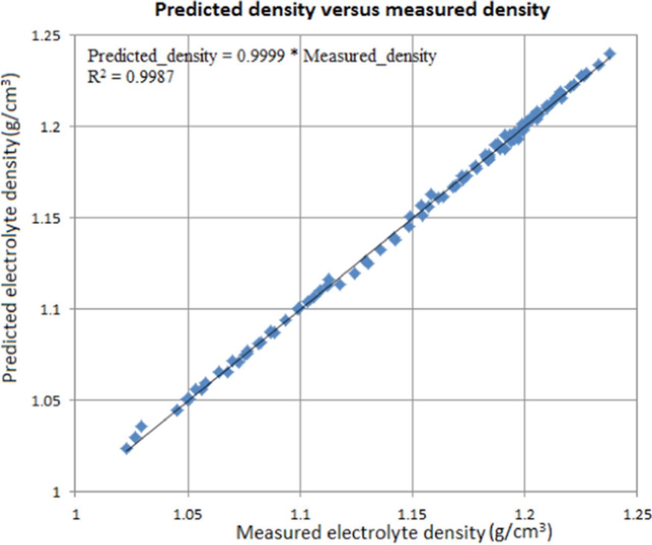
Figure 3. Fitting plot of predicted electrolyte density versus measured electrolyte density.
The volume force for the fluid was determined by multiplying Eq. 23 by the gravitational constant and applying it in the negative z direction.
![Equation ([24])](https://content.cld.iop.org/journals/1945-7111/162/14/E338/revision1/d0024.gif)
where Fz is the volume force in the z direction, ρ is the fluid density, and g is the gravitational constant.
The dynamic viscosity of the fluid was estimated by the following empirical equation, which is based on the experimental data from Price and Davenport:22
![Equation ([25])](https://content.cld.iop.org/journals/1945-7111/162/14/E338/revision1/d0025.gif)
where μ is the dynamic viscosity in Pa*s, [Cu] is the localized cupric ion concentration in mol/m3, CH2SO4 is the initial H2SO4 concentration in Kg/m3, and T is the absolute temperature in Kelvin. The fitting plot for the dynamic viscosity is shown in Figure 4.

Figure 4. Fitting plot of predicted dynamic viscosity versus measured dynamic viscosity.
The inner top face of the cell was set to have a wall slip boundary condition,18 due to the absence of a wall on the cell top.
![Equation ([26])](https://content.cld.iop.org/journals/1945-7111/162/14/E338/revision1/d0026.gif)
![Equation ([27])](https://content.cld.iop.org/journals/1945-7111/162/14/E338/revision1/d0027.gif)
where
v
is the fluid velocity vector,  is the unit normal vector to the inner top face, and μ is the dynamic viscosity.
The inlet face was set to have the flow rate in the designed boundary conditions (Table I), with the inflow electrolyte having the initial concentrations of cupric ion, sulfate ion, and hydrogen ion.
Table I. Boundary conditions used in the simulation.
| Inlet Flow Rate (ml/min) | Temperature (°C) | Current Density (A/m2) |
|---|---|---|
| 3.5 | 50 | 225 |
| 11 | 50 | 225 |
| 11 | 50 | 375 |
| 11 | 70 | 225 |
The outlet conditions were specified by prescribing a pressure on the outlet face without viscous stress:18
![Equation ([28])](https://content.cld.iop.org/journals/1945-7111/162/14/E338/revision1/d0028.gif)
![Equation ([29])](https://content.cld.iop.org/journals/1945-7111/162/14/E338/revision1/d0029.gif)
where μ is the dynamic viscosity, v is the fluid velocity vector, I is the identity tensor,  is the unit normal vector to the outlet face, and po is the pressure at the outlet.
All other faces were set to have a no slip wall boundary condition:18
![Equation ([30])](https://content.cld.iop.org/journals/1945-7111/162/14/E338/revision1/d0030.gif)
where v is the fluid velocity vector.
The drag force on an impurity particle was set to follow Stokes' law:
![Equation ([31])](https://content.cld.iop.org/journals/1945-7111/162/14/E338/revision1/d0031.gif)
where F is the drag force vector, mp, ρp, dp,  are the mass, density, diameter, velocity vector of thparticle,. is the velocity vector of the fluid, and μ is the dynamic viscosity.18
The gravity force and the buoyancy force on a particle is expressed as:
![Equation ([32])](https://content.cld.iop.org/journals/1945-7111/162/14/E338/revision1/d0032.gif)
where Fz is the sum of the two forces in the z direction, ρp and Vp are the density and volume of the particle, and ρf is the density of the fluid.
The inlet and outlet of particles are the same as the fluid flow. From the inlet plane, 10000 particles were unifory released at each step from t = 0 s to t = 18000 s with a step interval of 500 s. Their initial velocities are set to be governed by the fluid flow velocity field.
Particles that strike a wall would have a "freeze" condition, which means that they would be frozen at the posre they hit the wall with their final velocities equal to the particle velocities when striking the wall.
The electrorefining process was simulated under four different boundary condition combinations with varying inlet flow rate, temperature, and current density to understand the effects of inlet flow rate, temperature, and current density on impurity particle behavior in electrolyte. Table I shows the 4 different boundary conditions set in the simulations. Table II shows the main parameters used in the model, including key parameters for electrodepositionfluid flow, and impurity particle properties.
Mesh setting
The Model in this study discretized the domains (including the electrorefining cell and pipes) into tetrahedral mesh elements as shown in Figures 5a–5b. The maximum element size in the model was 0.0053 m, the minimum element size was 0.001 m, and the maximum element growth rate was set to be 1.13, as shown in Figure 5a.
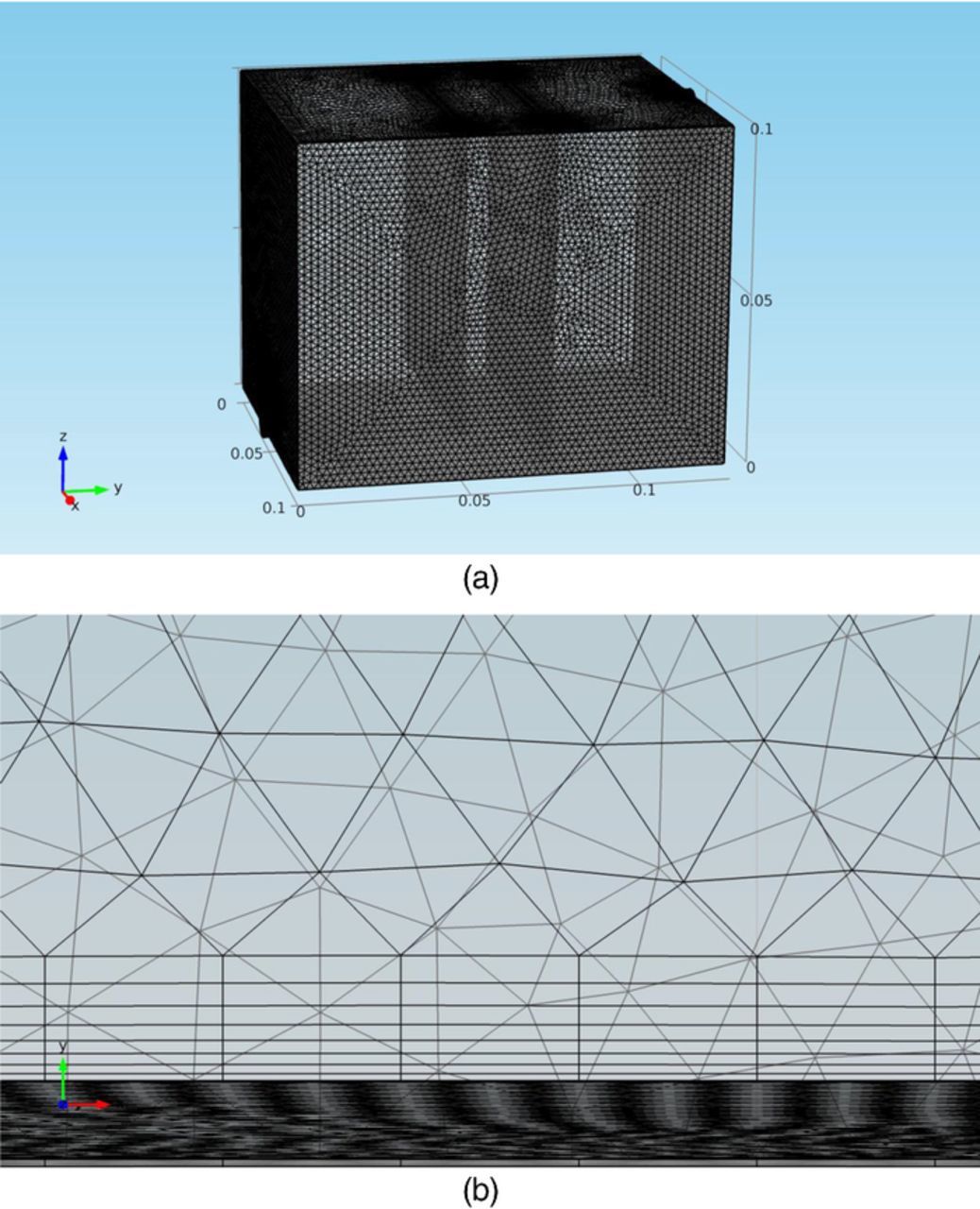
Figure 5. (a) Model mesh for the copper electrorefining cell defined in Model geometry section. (b) Boundary layer meshes at the anode surface boundary in the copper electrorefining cell defined in Model geometry section.
There were finer structured layers of elements along all surface boundaries. These layers of finer elements were integrated into the existing tetrahedral mesh elements in the 3D model. There were two boundary layers over each boundary, with the first layer thickness set at 0.00129 m and the second layer thickness to be 0.00155 m. Along surface boundaries of the anode and cathode front side faces (shown in Figure 5b), there were eight even finer layers of elements, with the first layer thickness to be 0.0001 m and a boundary layer stretching factor of 1.2 (the thickness increases by 20% from one layer to the next).
These geometry boundaries are discretized into triangular boundary elements. On all the boundaries in the model, these triangular boundary elements had a maximum element size of 0.0023 m, a minimum element size of 0.00015 m, and a maximum element growth rate of 1.08. The edges and vertices in the geometry are discretized into edge elements and vertex elements respectively.
The current cell meshes are the result of several mesh refinement through the development of the model and the simulation results from the current meshes do not show appreciable difference from those from the last meshes of coarser quality.
Simulation Results and Discussion
The electrodeposition, fluid flow, and impurity particle transportation processes were simulated in the model and the following results were obtained in the forms of line plots and three dimensional plots. The time-dependent simulations of current distribution and fluid flow field from 0 s to 18000 s had results almost at steady state with tiny changes after t = 5000 s. The further stationary simulations of current distribution and fluid flow field gave the steady state solutions for different boundary conditions, which are presented below. The simulations of impurity particle motions in the flowing electrolyte were time dependent from 0 s to 18000 s and the results of particle distributions in front of the cathode at 18000 s for different boundary conditions are presented.
First of all, the copper concentration distribution in the cell and the associated copper concentration profile between the electrodes at steady state under 11 ml/min, 50°C, and 225 A/m2 are shown in Figure 6a as an example and selected concentration/concentration difference statistics among the four boundary condition sets are shown in Figure 6b.
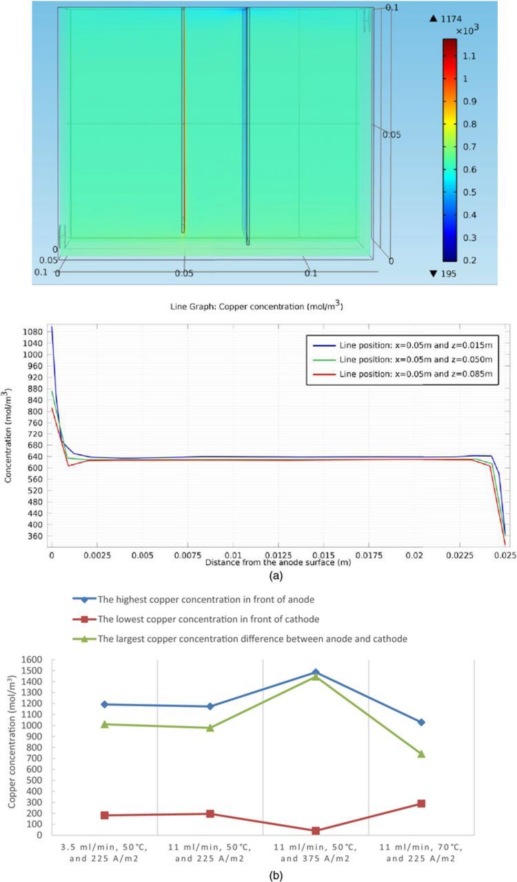
Figure 6. (a) Cu2+ concentration profile at steady state under conditions of 11 ml/min, 50°C, and 225 A/m2, in the copper electrorefining cell defined in Model geometry section (the color expresses the magnitude of localized Cu2+ concentration) and the associated copper concentration profile between the anode (the left side) and the cathode (the right side). (b) Selected copper concentration/concentration difference statistics at steady state under four sets of boundary conditions, in the copper electrorefining cell defined in Model geometry section.
As shown in the plots, the cupric ion concentration levels near anodes are much higher than that near cathodes, which results from the fact that copper is dissolved at the anode and recovered at the cathode. Among four sets of boundary conditions, there are some differences in the resulting copper concentrations. The general difference between the copper concentration near the anode and copper concentration near the cathode is highest under the condition of 11 ml/min, 50°C, and 375 A/m2, followed by 3.5 ml/min, 50°C, and 225 A/m2; 11 ml/min, 50°C, and 225 A/m2; and 11 ml/min, 70°C, and 225 A/m2.
During the electrorefining process, cupric ions are liberated from the anode and recovered along the cathode, but the diffusion rate is not high enough to transport cupric ions away from the anode diffusion layer and into the cathode diffusion layer. As a result, the cupric ions will be accumulated near the anode and depleted near the cathode, leading to the concentration differences between the electrodes. It is apparent that the higher the current density, the larger the concentration differences. When the inlet flow rate is raised from 3.5 ml/min to 11 ml/min, the convection between the electrodes is larger, resulting in smaller concentration differences. When the temperature is increased to 70°C, the diffusivity coefficient is larger according to Eq. 21, resulting in a higher diffusion rate and smaller concentration differences between the electrodes.
The fluid density profile in the cell is directly determined by the cupric ion concentration distribution and the density distribution on a slice 100 microns away from the front surface of the cathode is shown, which is important in this study. The density profiles in front of the cathode can significantly influence the fluid flow near the cathode front surface, which then affects the motion of impurity particles. Figure 7a shows the fluid density results at steady state and the associated quantified fluid density profile between the left and right edges of the cathode at the top and bottom of the slice for the boundary condition of 11 ml/min, 50°C, and 225 A/m2 as a representative. Figure 7b shows the selected electrolyte density/density gradient statistics among different boundary conditions.
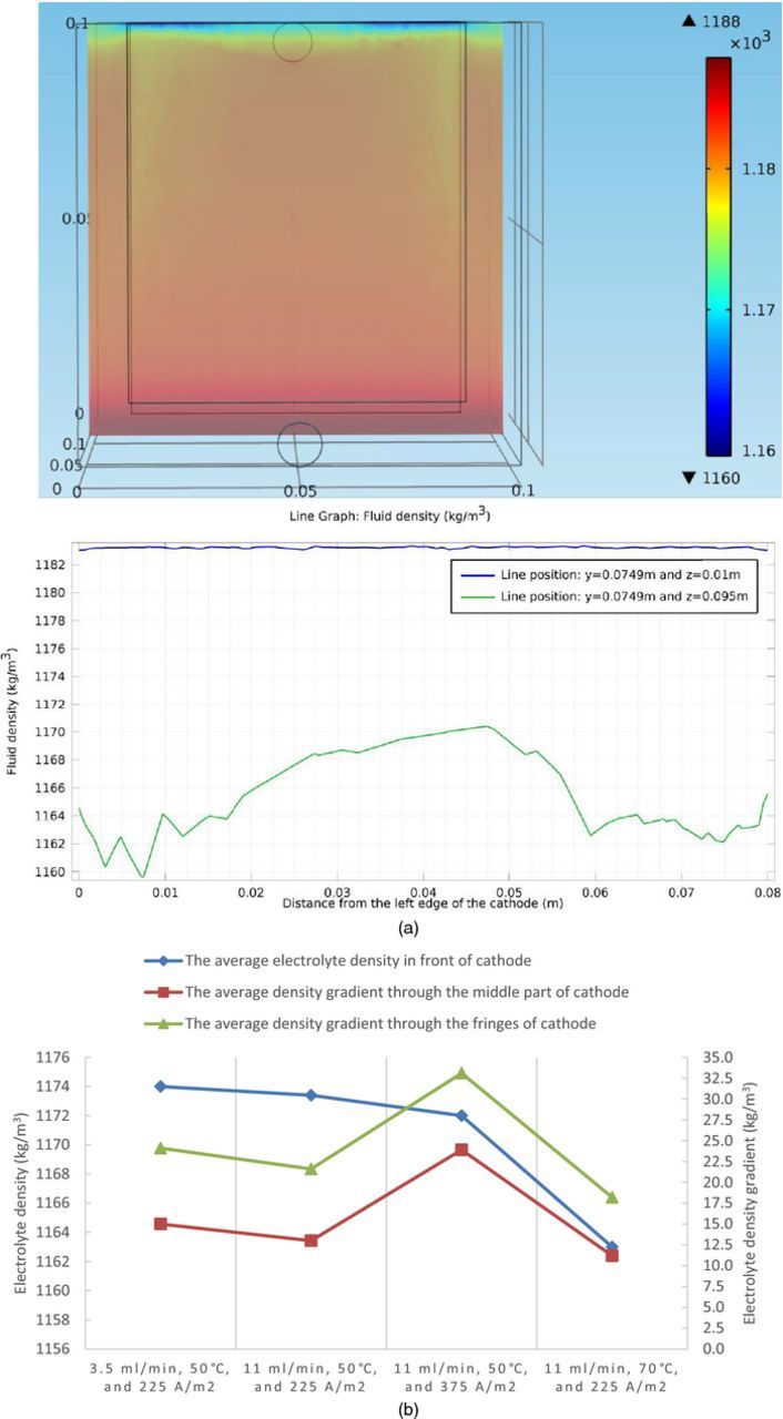
Figure 7. (a) Fluid density distribution on a slice 100 microns away from the front surface of the cathode at steady state under conditions of 11 ml/min, 50°C, and 225 A/m2, in the copper electrorefining cell defined in Model geometry section (the color expresses the magnitude of localized electrolyte density) and the associated quantified fluid density profile between the left and right edges of the cathode at the top and bottom of the slice. (b) Selected electrolyte density/density gradient statistics at steady state under four sets of boundary conditions, in the copper electrorefining cell defined in Model geometry section (the average electrolyte densities in front of cathode are plotted using the left Y-axis and the average density gradients through the middle part and the fringes of the cathode are plotted using the right Y-axis).
Notice that there are gaps between the cathode and the cell walls on the left, right, and bottom parts of the slices. Note that there are two rectangles with black borders, with the smaller one representing the anode and the larger one representing the cathode. Furthermore, there are major density gradients between the anode and the cathode (not shown in the graphs), which are obvious and can be deduced from the concentration profiles in the cell. It is the density gradients between the electrodes that drive the loop-shaped convection (Figure 8a). The density profiles above show that there are density gradients along the z direction in front of the cathode. It is important to point out that the density gradients in front of the fringes of the cathode are larger than those in front of the middle part of the cathode under all four sets of boundary conditions. The same case applies for the anode (not shown in the graphs), except the opposite density gradients direction. This means that the looping flow between the electrodes driven by density gradients is very likely to be faster through the two sides than through the middle part of the electrodes.
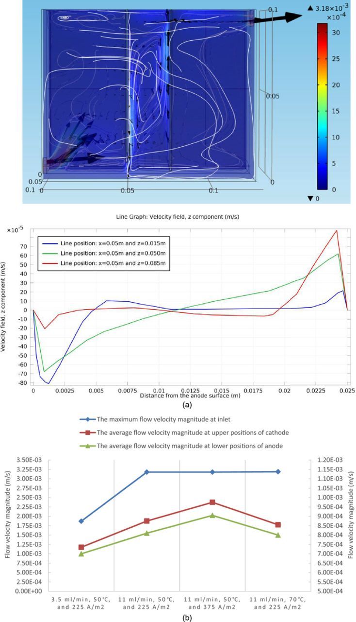
Figure 8. (a) Fluid flow velocity field at steady state under conditions of 11 ml/min, 50°C, and 225 A/m2, in the copper electrorefining cell defined in Model geometry section (the color expresses the magnitude of fluid velocity, the black arrows represent velocity vectors, and the white lines are streamlines) and the associated z component of fluid velocity profile between the anode (the left side) and the cathode (the right side). (b) Selected flow velocity magnitude statistics at steady state under four sets of boundary conditions, in the copper electrorefining cell defined in Model geometry section (the inlet maximum flow velocity magnitudes are plotted using the left Y-axis and the average flow velocity magnitudes at upper positions of cathode and lower positions of anode are plotted using the right Y-axis).
The density distributions are slightly different among four different sets of boundary conditions. As discussed before, higher inlet flow rate will intensify convection between the electrodes and therefore help abate the concentration differences, resulting in smaller density gradients. This is why the electrolyte density gradients under conditions of 11 ml/min, 50°C, and 225 A/m2 is smaller than that under conditions of 3.5 ml/min, 50°C, and 225 A/m2.
When the current density is increased from 225 A/m2 to 375 A/m2 as shown in Fig. 7b, it is obvious that density gradients in front of the cathode increase due to the intensified accumulation of cupric ions in the diffusion layer in front of the anode and the depletion of cupric ions in front of the cathode.
When the temperature is increased from 50°C to 70°C as shown in Fig. 7b, the electrolyte densities decrease as the temperature goes up. Moreover, the diffusivity coefficient for each ion, especially the cupric ion, is significantly increased, according to Eq. 21. Consequently, the diffusion rate is much higher removing more accumulated cupric ions in front of the anode and replenishing more cupric ions to the diffusion layer in front of the cathode, which makes the density distribution of the depletion region more uniform. As a result, the density gradients are smaller under higher temperature as shown in Fig. 7b.
The fluid velocity field in the cell is driven by both the inlet inflow and the density gradients between the electrodes. Figure 8a shows the fluid velocity field at steady state in the entire cell and the associated z component of fluid velocity profile between the electrodes for the boundary condition of 11 ml/min, 50°C, and 225 A/m2 as a representative. Figure 8b presents the selected fluid flow velocity magnitude statistics among different boundary condition sets.
As shown in Figure 8a, the fluid comes from the inlet, goes into the cell with a set velocity, and then encounters the anode. Part of the fluid goes up along the left side of the anode and forms loops in the left part of the cell. Another part of the fluid flows through the gaps between the side edges of the electrodes and the cell walls, and enter into the right part of the cell. The rest of the fluid enters the domain between the electrodes from the bottom and side gaps between the edges of the anode and the cell walls. The electrolyte in between the electrodes flows along loop-shaped paths influenced by both the density gradients and the inlet inflow. Then some of it exits the loops at the bottom and enters the right part of the cell. Finally, the fluid flows out of the cell through the outlet by pressure. This is the general fluid velocity pattern observed in all boundary condition sets. However, as conditions vary, the fluid flow velocity field changes accordingly.
Several observations can be made from the Figures 8a–8b. Firstly, the electrolyte comes with larger velocities through the inlet, when the inlet flow rate is increased from 3.5 ml/min to 11 ml/min. Secondly, velocity magnitudes of the flow field between the electrodes (the looping flow) are affected by both the density gradients between the plates and the inlet flow rate. At the low flow rate condition (3.5 ml/min), the flow velocities are comparatively small. While at the high flow rate condition (11 ml/min), the fluid flow in the cell is intensified and the flow between the electrodes is more influenced by the incoming flow from the bottom and side gaps. According to Figure 8b, this results in flow with larger velocities between the electrodes, though the density gradients decrease a little. Furthermore, at higher current density condition (375 A/m2), since the density gradients between the electrodes are larger, the flow field generated has larger velocities. Finally, when the temperature is increased from 50°C to 70°C, the flow velocities will increase due to lower fluid viscosity, but the density gradient, which turns out to be the dominant factor, becomes smaller, due to significantly increased diffusivity of cupric ion. Therefore, the velocities of the flow field are decreased.
Since the flow velocity field near the cathode is not shown in detail in Figure 8a, which is presented to mainly show general flow pattern in the cell, a slice of velocity field 100 microns away from the front surface of the cathode, which determines the motion of impurity particles near the cathode front surface, is shown for the boundary condition set of 11 ml/min, 50°C, and 225 A/m2 as a representative (Figure 9a), as a complement to Figure 8a. Figure 9b presents the variation of the average z component velocity magnitude in front of cathode among four boundary condition sets.
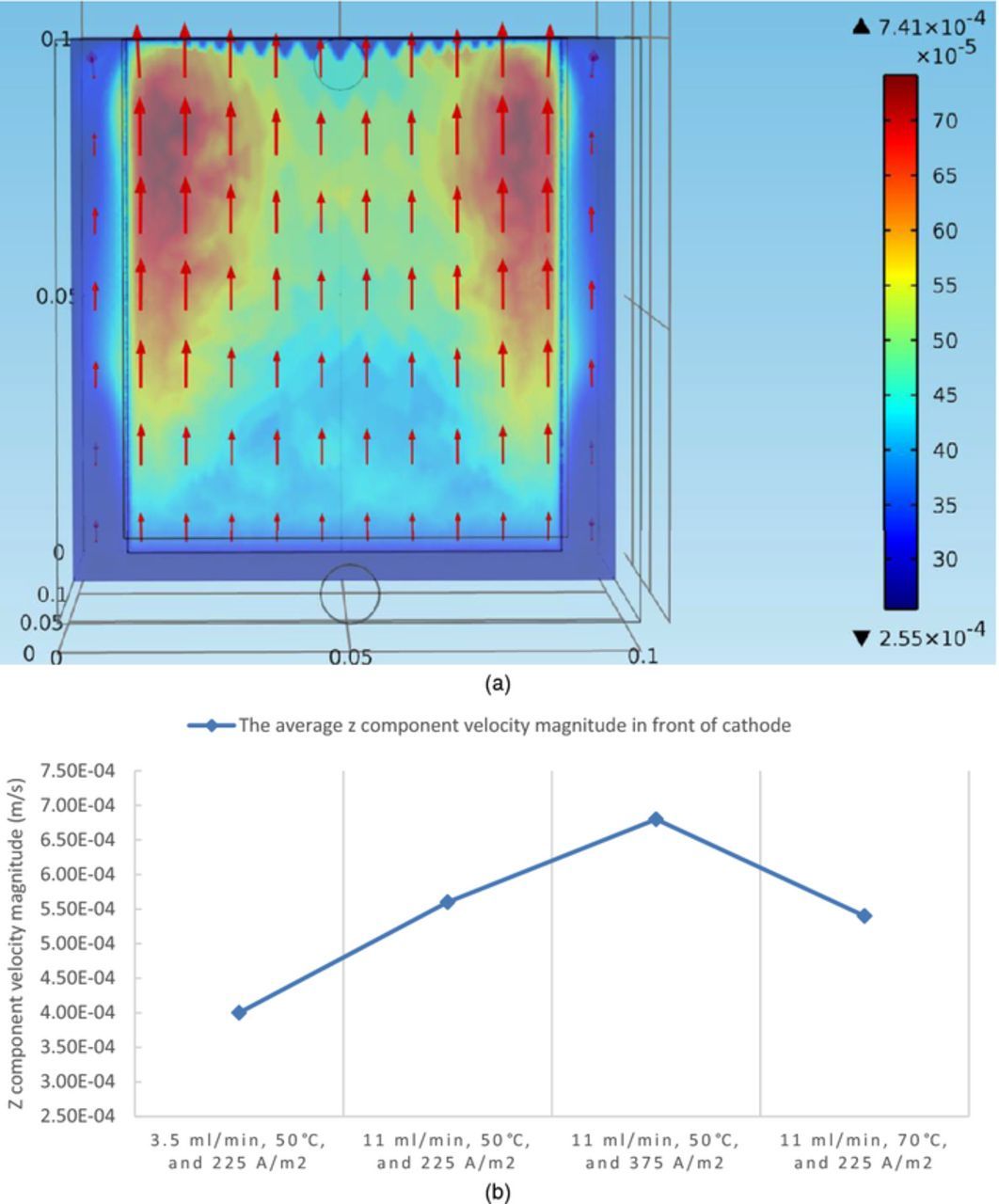
Figure 9. (a) The fluid velocity field on a slice 100 microns away from the front surface of the cathode at steady state under conditions of 11 ml/min, 50°C, and 225 A/m2, in the copper electrorefining cell defined in Model geometry section (the arrows represent velocity vectors and the color expresses the magnitude of the z component of fluid velocity). (b) The average z component velocity magnitude in front of cathode at steady state under four sets of boundary conditions, in the copper electrorefining cell defined in Model geometry section.
Similarly to the fluid density distribution figures, in Figure 9a, there are gaps between the cathode and the cell walls on the left, right, and bottom parts of the slices, where the z components of fluid velocities are relatively small.
It is apparent that most fluid velocity vectors are almost vertical, which means they are nearly along the z direction and have almost no x and y components. Another significant finding is that the z components of fluid velocities are almost all in the positive direction and their magnitudes are larger in front of the fringes of the cathode, than in front of the middle part of the cathode. This should result from the density gradients difference between the two areas. Furthermore, the z components of fluid velocities become larger gradually along the positive z direction, resulting from the density gradients along that direction.
As shown in Figure 9b, the z components of fluid velocities near the cathode are generally the smallest under conditions of 3.5 ml/min, 50°C, and 225 A/m2, and are higher when the inlet flow rate is increased to 11 ml/min, due to the intensification of the flow. When the current density is raised from 225 A/m2 to 375 A/m2, they are increased, due to the larger density gradients. When the temperature is increased from 50°C to 70°C, they are decreased, because of the smaller density gradients due to significantly increased diffusivity of cupric ion, despite lower viscosities.
The motion of impurity particles in front of the cathode needs to be discussed. In order to understand this, how the particles are transported to the cathode needs to be understood. Figures 10a–10d show the general motion of the particles in the cell from four moments in the electrorefining simulation process. Notice that the particles were injected from the inlet every 500 seconds. As a result, Figure 10a shows only the position distribution of the first group of particles injected in the burst at t = 0 s; Figure 10b shows the position distributions of two groups of particles (one injected at t = 0 s and the other one injected at t = 500 s); Figure 10c shows three superimposed groups of particles, injected at t = 0 s, t = 500 s, and t = 1000 s, respectively; and four superimposed groups of impurity particles injected at t = 0 s, t = 500 s, t = 1000 s, and t = 1500 s, respectively are shown in Figure 10d. Due to the relatively large time interval between injection bursts, each group of particles can be distinguished clearly in the plots. Note that the motions of each group of particles in the cell are almost identical and the position distribution of one group of particles virtually represents the position distribution of the previous group of particles at the time point 500 seconds ago. Thus the position distributions of four groups of particles in Figure 10d can be considered as the particle trajectories of the first group of particles injected at t = 0 s.
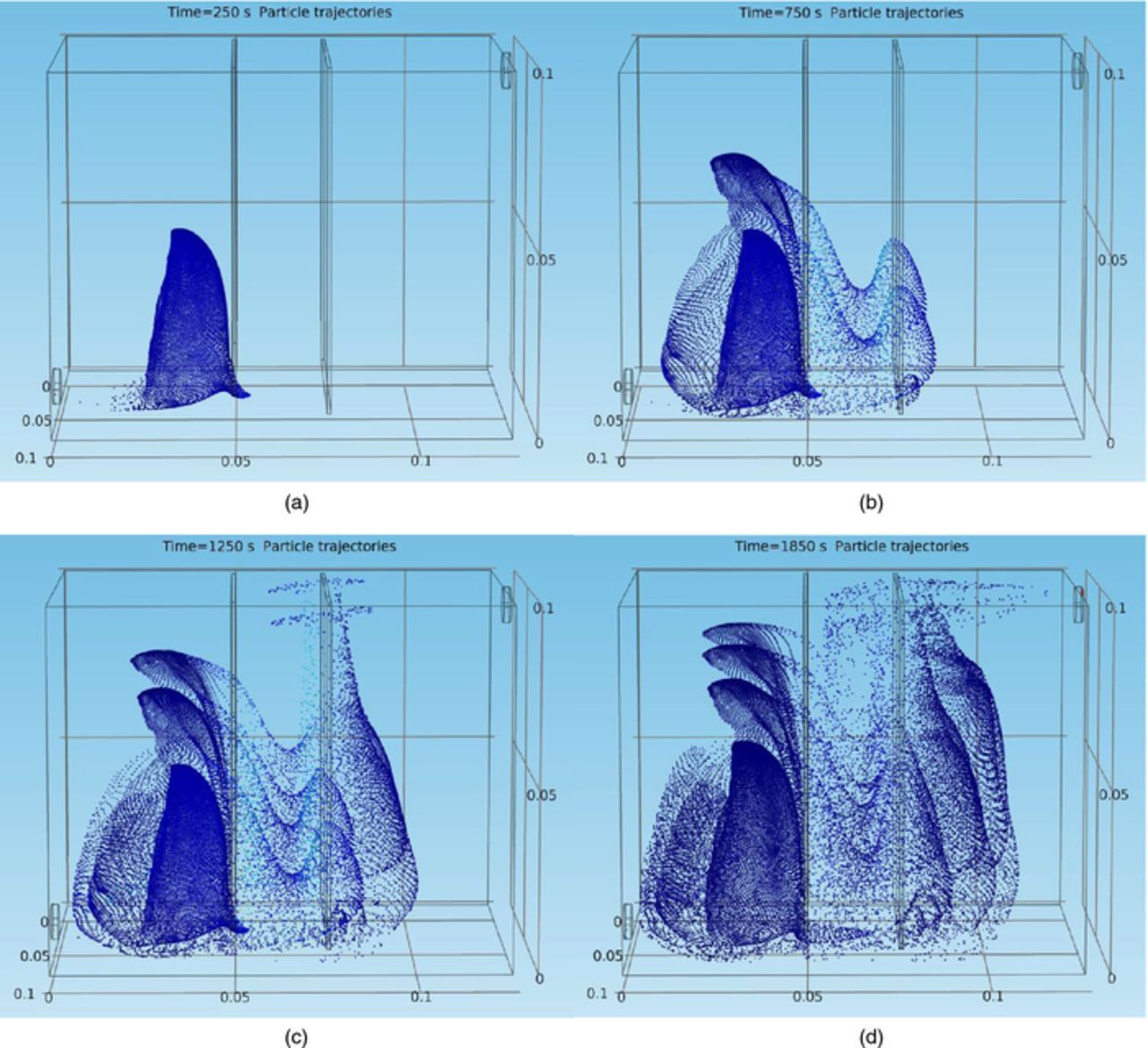
Figure 10. (a) & (b) Instantaneous particle (uniform size of 14.5 μm) position distributions at t = 250 s (left) and t = 750 s (right), under conditions of 11 ml/min, 50°C, and 225 A/m2, in the copper electrorefining cell defined in Model geometry section. (c) & (d) Instantaneous particle (uniform size of 14.5 μm) position distributions at t = 1250 s (left) and t = 1850 s (right), under conditions of 11 ml/min, 50°C, and 225 A/m2, in the copper electrorefining cell defined in Model geometry section.
The motion of these particles is determined by Newton's second law and is driven by both drag force based on Stokes' law and the gravity force. Therefore, the electrolyte flow velocity field exerts great effect on their motion. As a result, after the particles enter the cell from the inlet, some of the particles move along similar loops in the left part of the cell as the fluid flow. Some of them flow into the domain between the electrodes and approach the cathode through the gaps between the side edges of the anode and the cell walls, while another part of them flow over the domain and enter into the right part of the cell through the gaps between the side edges of the cathode and the cell walls. The rest of the particles go into this middle domain and come close to the cathode through the gap between the bottom edge of the anode and the cell bottom wall. As some of these particles approach the cathode, some of them will settle down and the other of them will go up along the cathode surface and suspend in the electrolyte. Particles suspended in the middle domain would move along loops between the electrodes. Some of these particles exit the loops at the bottom of the domain and enter into the right part of the cell, eventually leaving the cell through the outlet. Whether a particle in a position close to the cathode will suspend or settle down depends on the superposition of the settling velocity of the particle and the z component of the localized flow velocity. Since the concentration of the particles is extremely low compared to other species, we can assume that the motion of each particle is not influenced by other particles. Thus, for dilute suspensions and laminar flow, Stokes' law predicts the settling velocity of small spheres in fluid. Based on Stokes' law, the settling velocity is given by:
![Equation ([33])](https://content.cld.iop.org/journals/1945-7111/162/14/E338/revision1/d0033.gif)
where V is the settling velocity, ρ is density (the subscripts p and f indicate particle and fluid respectively), g is the acceleration due to gravity, d is the diameter of the particle and μ is the kinematic viscosity of the fluid.23
In this equation, the density and the diameter of the impurity particle are known parameters (4200 kg/m3 and 14.5 μm, respectively in this study, as shown in Table II). According to Figure 7b, the average density of the electrolyte on the cross section 100 microns away from the front surface of the cathode varies from 1163 kg/m3 to 1174 kg/m3, so we can assume the electrolyte density is 1170 kg/m3. The dynamic viscosity of the fluid can be estimated by the empirical equation based on our laboratory measurements:
![Equation ([34])](https://content.cld.iop.org/journals/1945-7111/162/14/E338/revision1/d0034.gif)
where μ is the dynamic viscosity in centipoise, and T is the temperature in degree C.
Therefore, the settling velocity for the impurity particles can be calculated for both temperature conditions. Table III shows the results.
Table III. Calculated settling velocity for high and low temperatures.
| Temperature | Settling Velocity (m/s) |
|---|---|
| High Temperature (70°C) | 4.18E-04 |
| Low temperature (50°C) | 3.03E-04 |
The z components of fluid velocities in positions close to the cathode for four sets of boundary conditions were computed through the model and are shown in Figures 9a–9b. Then the net z direction velocities of the impurity particles at steady state on a slice 100 microns away from the front surface of the cathode can be computed, which are shown in Figure 11a for the boundary condition of 11 ml/min, 50°C, and 225 A/m2 as a representative. Particles with positive net z direction velocities tend to suspend in the electrolytic solution, while particles with negative net z direction velocities have the tendency to settle down to the bottom of the cell.
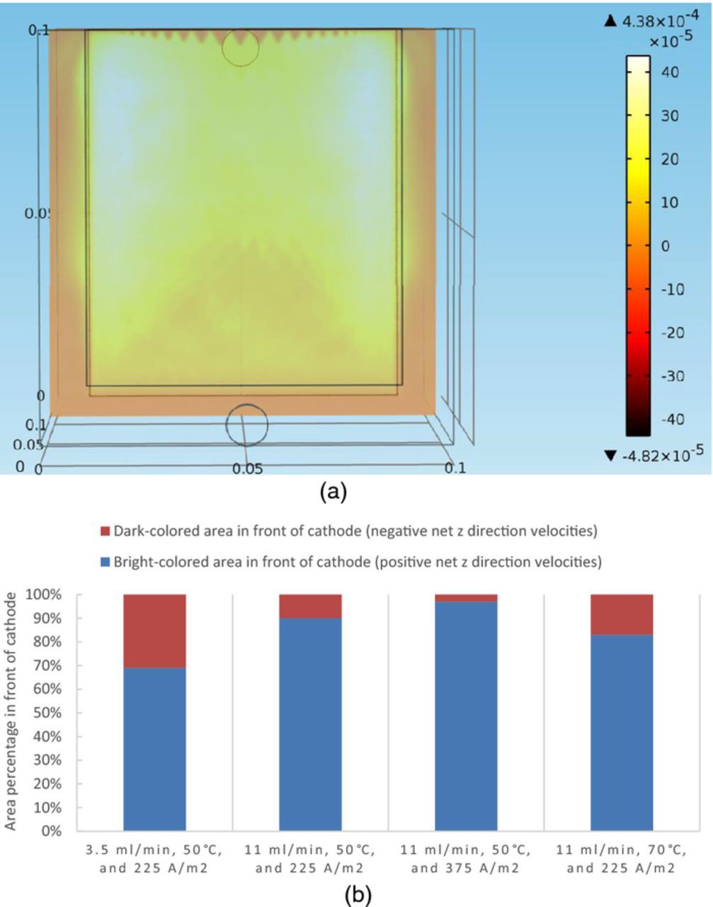
Figure 11. (a) The net z direction velocities of impurity particles at steady state on a slice 100 microns away from the front surface of the cathode under conditions of 11 ml/min, 50°C, and 225 A/m2, in the copper electrorefining cell defined in Model geometry section. (b) Percentages of dark-colored and bright-colored areas in front of cathode at steady state under four sets of boundary conditions, in the copper electrorefining cell defined in Model geometry section.
Similarly to previous figures, there are gaps between the cathode and the cell walls on the left, right, and bottom parts of the slices, where the net z direction velocities of impurity particles are not pertinent to the electrode surface contamination.
Because of the symmetric color range setting in the figure, it is clear that a dark-colored area representing negative net z direction velocities is in front of the lower middle area of the cathode. While in front of the fringes of the cathode, there is a bright-colored area representing positive net z direction velocities. The brighter the color, the larger the net z direction velocities of impurity particles; and the darker the color, the smaller the net z direction velocities. Figure 11b presents the percentages of bright-colored and dark-colored areas under each set of boundary conditions. When the inlet flow rate is raised from 3.5 ml/min to 11 ml/min, the dark-colored area shrinks and the bright-colored area expands from the fringes to the middle. Also, when the current density is increased from 225 A/m2 to 375 A/m2, the net z direction velocities on the slice increase. When the temperature is raised from 50°C to 70°C, the dark-colored area expands from the lower middle area to the fringes and the net z direction velocities on the slice decrease.
The proposed theory is that larger particles with higher settling velocities settle to the bottom of the cell, but smaller particles with lower settling velocities remain in suspension, providing them with more opportunities to be incorporated into the cathodic deposit. Conversely, larger particles with a higher settling velocity will be removed from suspension more rapidly, and hence be less likely to be co-deposited. In this simulation, although the particle size is fixed, temperature has significant effect on the settling velocities of the particles and thus affects the net z direction velocities of the particles. Besides, inlet flow rate, current density, and temperature together influence the fluid velocity field in front of the cathode, and therefore play key roles in determining the net z direction velocities of the particles.
When impurity particles get close to the cathode, those with positive net z direction velocities have the tendency to go up and remain in suspension, while those with negative net z direction velocities tend to fall down and settle to the bottom of the cell. Consequently, at the condition of 3.5 ml/min, 50°C, and 225 A/m2, the number of particles suspended would be the smallest and should be correlated with the highest cathode purity. At the condition of 11 ml/min, 50°C, and 375 A/m2, the number of particles remaining in suspension would be the largest and should be correlated with the most contaminated cathode, followed by the condition of 11 ml/min, 50°C, and 225 A/m2, and then the condition of 11 ml/min, 70°C, and 225 A/m2.
At last, the impurity particle distribution maps on a slice with the identical area as the cathode, 100 microns away from the front surface of the cathode at t = 18000 s, are shown for four sets of boundary conditions in Figures 12a–12d. The number of impurity particles was counted from the simulation results by COMSOL for the four corner positions and the center position, which are shown in Table IV.
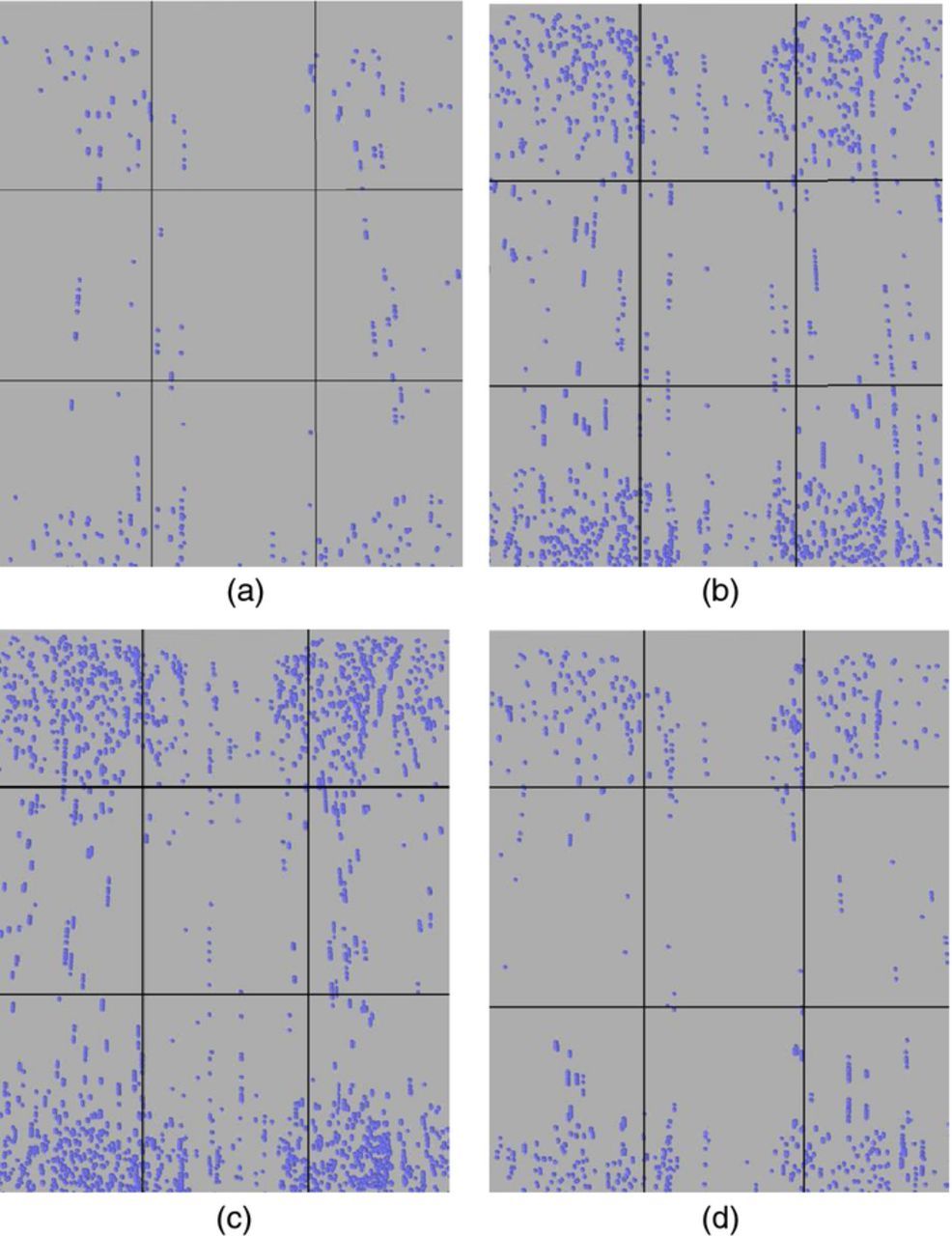
Figure 12. (a) – (d) Impurity particle distribution maps on a slice 100 microns away from the front surface of the cathode at t = 18000 s, divided into 9 sections. (a) 3.5 ml/min, 50 °C, 225 A/m2 (b) 11 ml/min, 50 °C, 225 A/m2 (c) 11 ml/min, 50 °C, 375 A/m2 (d) 11 ml/min, 70 °C, 225 A/m2.
Table IV. Impurity particle counts at certain sections for each set of conditions.
| Section | Left up corner | Right up corner | Center | Left down corner | Right down corner |
|---|---|---|---|---|---|
| 3.5 ml/min, 50°C, 225 A/m2 | 39 | 31 | 9 | 43 | 50 |
| 11 ml/min, 50°C, 225 A/m2 | 273 | 278 | 48 | 291 | 302 |
| 11 ml/min, 50°C, 375 A/m2 | 446 | 423 | 51 | 486 | 494 |
| 11 ml/min, 70°C, 225 A/m2 | 156 | 145 | 21 | 160 | 166 |
The calculated impurity densities are in accordance with the trends observed in the results of the net z direction velocities of impurity particles at steady state shown in Figures 11a–11b. The total number of particles on the map is the smallest at the condition of 3.5 ml/min, 50°C, and 225 A/m2, and is the largest at the condition of 11 ml/min, 50°C, and 375 A/m2. The total number of particles at the condition of 11 ml/min, 50°C, and 225 A/m2 is the second largest, corresponding to the second largest bright-colored area shown in Figure 11b. Similarly, since the bright-colored area under conditions of 11 ml/min, 70°C, and 225 A/m2 is the third largest, the total number of impurity particles under this set of conditions is also the third largest. Another reason why there are more particles under the condition of high inlet flow rate, than under the condition of low inlet flow rate, is that larger inlet flow can transport more particles to the bottom of the domain between the electrodes and therefore increase the number of suspended particles there. These particles can then be picked up by the recirculation between the plates.
It is noteworthy that, the number of particles at center section is much smaller than that at corner sections. This is partly because of the smaller net z direction velocities of particles at the center section and larger net z direction velocities at corners, according to Figure 11a. More importantly, the number of impurity particles on a position also depends on whether or not there is a high velocity pathway to that particular position. In an approximate way, from Figure 9a and Figure 11a, it can be deduced that there are high velocity upward pathways to corner positions and low velocity upward pathways to center positions. The relatively smaller number of particles in the edge-middle sections results from higher particle velocities and therefore shorter particle residence time in these two sections. In fact, the particle distribution maps are essentially cross-sections from the particle trajectories. At some positions in the maps, there are particles in lines, which show the effects of upward flow that drives particles moving upward in lines.
Figures 13a–13b show high/low velocity pathways in a more accurate way by directly showing particles' z components of velocities and the z direction positions (distance from bottom of the cell). More particles move into the inter-electrode domain through the gaps between the side edges of the anode and the cell walls, than through the gap between the bottom edge of the anode and the cell bottom wall as seen in the graphs. Note that this set of figures shows the particle distribution in the inter-electrode domain at an early stage (t = 3000 s) when particles do not have enough time to flow into the middle part of the domain. As shown in the graphs, there are much more particles moving along the loops in the two side parts of the domain between the electrodes than in the middle part of the domain. Most of the impurity particles moving in the middle part of the domain have settled to the bottom of the cell, and only a small portion of these particles still flow along the loops between the electrodes. As seen in Figure 13a, in the two side parts of the domain, most particles are moving upward (yellow and orange color) along the cathode, then flowing horizontally (green color) from the cathode to the anode, then moving downward (blue color) along the anode, finally flowing horizontally (green color) back to the cathode. Nevertheless, for particles in the middle part of the domain, most of them are green/yellow, indicating that they do not move in loops. From Figure 13b, it is apparent that most of the particles in the middle part of the domain are resting on the bottom of the cell (dark blue color), with only a small portion of them still flowing between the electrodes above the bottom cell wall. This shows that most particles in the middle part settle to the bottom and only a few of them remain in suspension. On the other hand, for particles in the two side parts of the domain, most of them are suspended above the bottom of the cell and only a small portion of them settle to the bottom. This demonstrates that there are much less opportunities for particles to deposit on the cathode in the middle part of the domain than in the side parts of the domain at early stages and explains partly why there are more particles distributed at corner sections than at the center section in Figures 12a–12d. This also demonstrates smaller net z direction velocities of particles in front of the middle part of the cathode and lower velocity upward pathways through the middle part of the cathode. However, this only analyzes the situation at early stages and the particle distribution in the inter-electrode domain at later stages (such as 9000 s, 15000s, 18000 s) also needs to be examined to see if there are still less opportunities for particles to deposit at the center than at the corners of the cathode.
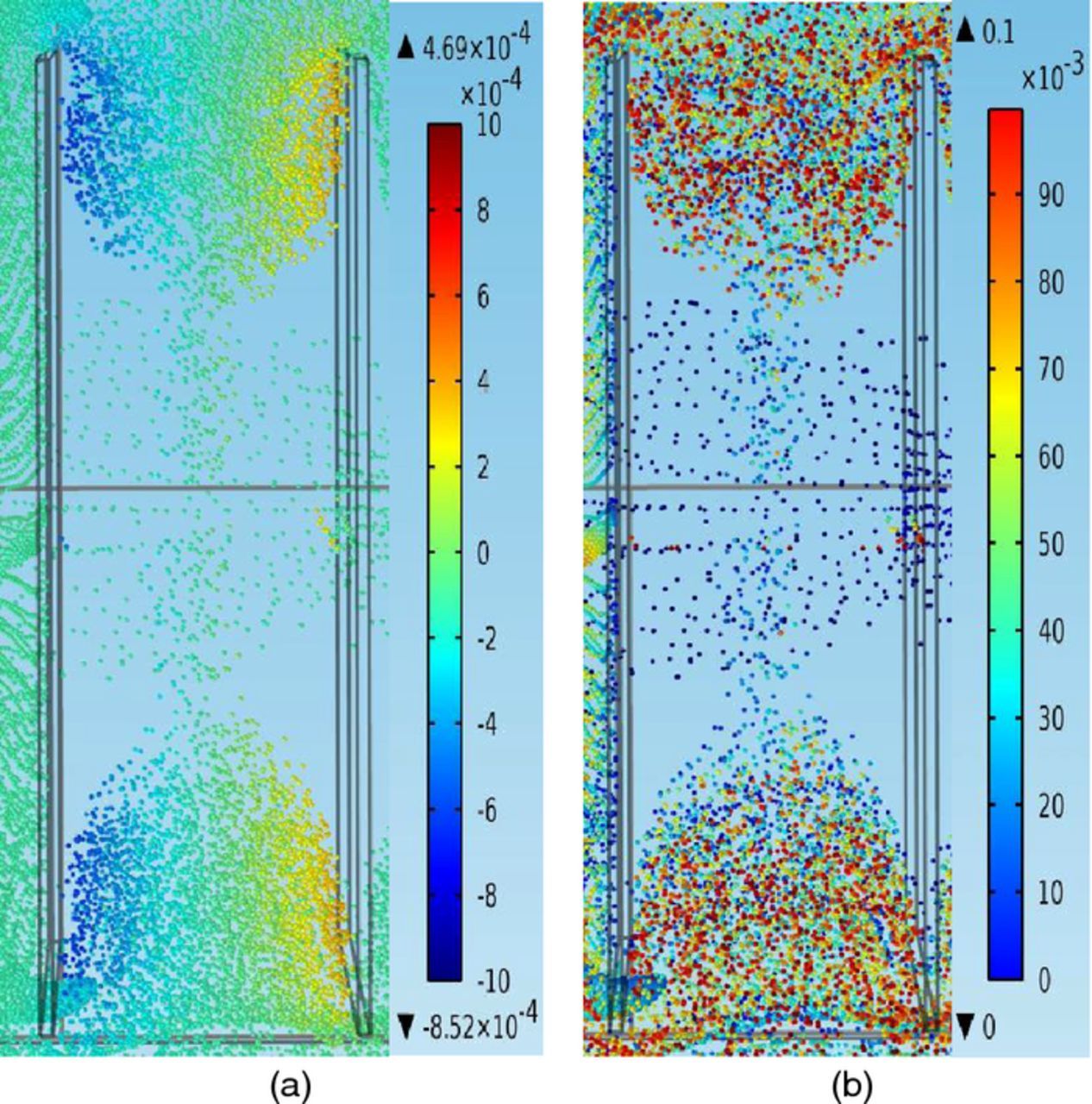
Figure 13. (a) – (b) Velocities and positions of impurity particles between the anode (left cuboid) and the cathode (right cuboid), from a bird's-eye top view, at t = 3000 s, under conditions of 11 ml/min, 50°C, and 225 A/m2, in the copper electrorefining cell defined in Model geometry section (the color expresses the magnitude of the z component of particle velocity for the left graph and expresses the magnitude of the z direction position of particle for the right graph). (a) The z components of particles velocities (m/s) (b) The z direction positions of particles (m).
As seen in Figures 14a–14b, much more impurity particles flow to the middle part of the domain at later stages. It is important to notice that there are two small vacancies between the particles and the front side surfaces of the electrodes, which indicates that particles at the middle part of the domain flow in loops with a larger distance from the electrodes than particles at the side parts of the domain. The closer to the middle line of the domain, the larger the distance from the electrodes and the less opportunities for particles to deposit on the cathode. As a result, it is still difficult for particles to deposit at the center part of the cathode. Similarly, this phenomenon is due to the smaller net z direction velocities of particles in front of the middle part than in front of the edge parts of the cathode and lower velocity upward pathways through the middle part than through the edge parts of the cathode. Consequently, particles in the middle part of the inter-electrode domain tend to flow in loops with certain distances away from the cathode so that larger net z direction velocities of particles and higher velocity upward pathways exist. Thus at later stages there are still less opportunities for particles to deposit at the center part than at the edge parts of the cathode and this also explains why there are more particles distributed at corner sections than at the center section in Figures 12a–12d.
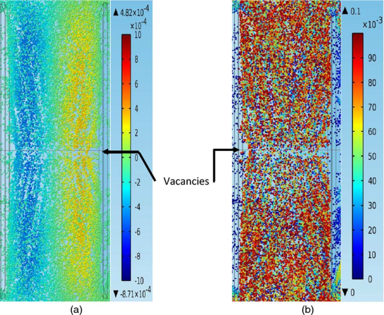
Figure 14. (a) – (b) Velocities and positions of impurity particles between the anode (left cuboid) and the cathode (right cuboid), from a bird's-eye top view, at t = 18000 s, under conditions of 11 ml/min, 50°C, and 225 A/m2, in the copper electrorefining cell defined in Model geometry section (the color expresses the magnitude of the z component of particle velocity for the left graph and expresses the magnitude of the z direction position of particle for the right graph). (a) The z components of particles velocities (m/s) (b) The z direction positions of particles (m).
When the impurity particles move into the range of 0.0001 m or shorter distance from the cathode, they are more likely to be transported and attached to the cathode surface and become co-deposited with copper as impurities in the final product. No matter what plays the key role in moving the particles to the cathode, their distribution on the cathode should be very close to that on the slice 100 microns away from the front surface of the cathode, due to this limited distance. Therefore, a basic idea of how impurity particles will be distributed on the cathode, as well as the impurity concentration distribution on the cathode, could be acquired from the impurity particle distribution maps in Figures 12a–12d.
In order to experimentally validate the simulation results from COMSOL, copper electrorefining experiments were performed twice under each of the four sets of conditions in the simulations.24 Titanium dioxide particles were added to the electrorefining cell from the inlet at a rate of 500 mg/l TiO2, to act as impurity particles. The particles have a density of 4200 kg/m3, with their sizes mostly distributed at 14.5 μm, as shown in Figure 15. All other parameters of the copper electrorefining experiments were the same as the simulation (Table II). After five hours (18000 s) of electrorefining tests, cathodes were harvested and the surface concentration of titanium dioxide impurity was analyzed at the corners and center of each cathode for comparison with the modeling. Laser-Induced Breakdown Spectroscopy (LIBS) was utilized to analyze the surface impurity concentration.25,26 The experimental results, corresponding with the results of the simulation, are shown in Table V.
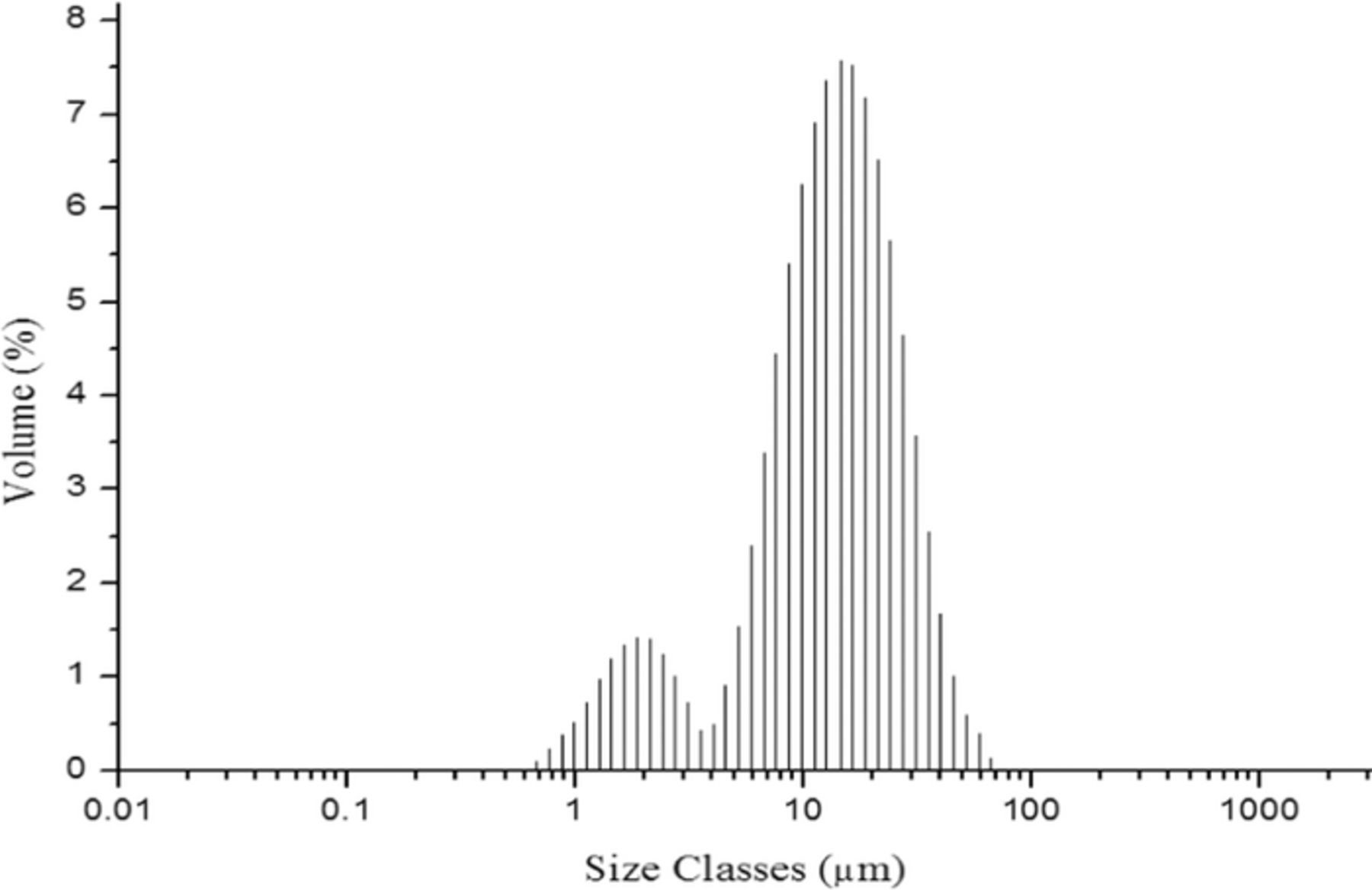
Figure 15. Particle size distribution (after 1 minute sonication) of TiO2 particles used in the copper electrorefining experimental tests (1 minute sonication of the particles was applied because the particles were sonicated before they were added to the electrorefining cell from the inlet).
Table V. Experimental and simulation results for each set of boundary conditions.
| Condition | Up corners average | Center | Down corners average | |
|---|---|---|---|---|
| 3.5 ml/min, 50°C, 225 A/m2 | Simulation (counts) | 35 | 9 | 46.5 |
| Experiment (concentration, weight percent) | 1.39% | 0.39% | 1.71% | |
| 11 ml/min, 50°C, 225 A/m2 | Simulation (counts) | 275.5 | 48 | 296.5 |
| Experiment (concentration, weight percent) | 7.72% | 3.73% | 8.00% | |
| 11 ml/min, 50°C, 375 A/m2 | Simulation (counts) | 434.5 | 51 | 490 |
| Experiment (concentration, weight percent) | 13.33% | 6.16% | 17.85% | |
| 11 ml/min, 70°C, 225 A/m2 | Simulation (counts) | 150.5 | 21 | 163 |
| Experiment (concentration, weight percent) | 5.69% | 1.43% | 6.33% |
To validate the simulation results, the impurity particle distribution maps on the slice 100 microns away from the front surface of the cathode were compared and correlated with experimental impurity data as shown in Figure 16, based on the data in Table V.
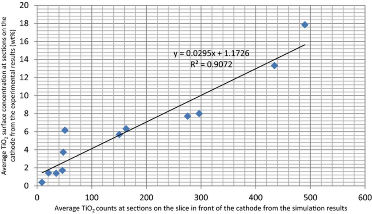
Figure 16. Correlation between the simulation results (impurity particle counts) and the experimental results (surface impurity concentration).
It can be seen that most points are close to the fitting line and thus the simulation results correlate with the experimental results well. Since the simulation results show a very good correlation, the impurity particle distribution maps on the slice in front of the cathode can be used to predict the impurity concentration distribution on the cathode in future copper electrorefining experiments with different process parameters by simply changing the boundary conditions in the model. Errors in the simulation may result from incomplete description of the experimental conditions, errors in determining the process parameters in the simulation, and errors in the approximation of the cathode to the slice in front of it, and etc.
Conclusions
According to the COMSOL simulation results, the copper concentration distribution, the electrolyte density distribution, the fluid velocity field, the impurity particle trajectories, and the impurity particle distribution, were influenced significantly by boundary conditions of inlet flow rate, temperature and current density. The impurity particle distribution maps on the slice 100 microns away from the front surface of the cathode are validated to a good extent, by the experimental data of the titanium dioxide impurity concentration on sections of the cathode. As a result, the simulation results of the particle distribution maps could be utilized to predict the impurity concentration distribution on the cathode obtained in copper electrorefining cell.
The z components of fluid velocities and the settling velocities of impurity particles, which are influenced by inlet flow rate, temperature, and current density, are believed to be the main factors that determine whether or not the particles settle or remain in suspension. Particles with a positive net z direction velocity (upward in the z direction) will suspend in the electrolyte, providing them with more opportunities to be incorporated into the cathodic deposit. Conversely, particles with a negative net z direction velocity (downward in the z direction) will settle and be removed from suspension more rapidly, and hence be less likely to be co-deposited. In addition, the number of impurity particles on a position is also dependent on whether or not there is a high velocity pathway to that particular position. These have been proven by the correlation of the simulation results of the net z direction velocities of particles, impurity particle distribution maps, and particle trajectories between the electrodes.
From the validated simulation results, process parameters in copper electrorefining can be optimized accordingly. Firstly, the inlet flow rate should be decreased as much as possible, although the minimum flow rate will be limited by the replenishment of additives such as thiourea and glue. If the flow rate is too low, the residence time of electrolyte becomes too long, leading to inadequate replenishment of additives. However, this may be solved by increasing the concentration of additives in the inflow electrolyte. Secondly, the cell temperature should be increased to higher values, though this will be limited by the tankhouse facility ability and high temperatures may raise other problems. Thirdly, the current density should be set as low as possible, though this is limited by the requirement of production. Lastly, cathode blanks should be made with a larger width to height ratio to decrease the effects of more contaminated fringes on the overall purity of copper cathode.
The effects of inlet flow rate, temperature, and current density on the impurity particles behavior in the electrolyte and their distribution on the slice, can be concluded as follows:
- (1)The inlet flow rate has the most influential effect on the particles behavior and their distribution. It has a positive correlation with the number of particles on the slice. Therefore the inlet flow rate should be set as low as possible, with higher additive concentrations in the inflow electrolyte.
- (2)The current density exerts a positive effect on the impurity particle counts on the slice 100 microns away from the front surface of the cathode. Thus it should be decreased to as low as possible with acceptable production rate.
- (3)There exists a negative correlation between the temperature and the number of particles on the slice, so the temperature should be raised to higher values.
- (4)The number of impurity particles at corner sections is apparently much larger than that at the center section, regardless of the boundary conditions. Therefore cathode blanks should be made with a larger width to height ratio.