


Abstract
The Galactic Plane Infrared Polarization Survey (GPIPS) seeks to characterize the magnetic field in the dusty Galactic disk using near-infrared stellar polarimetry. All GPIPS observations were completed using the 1.83 m Perkins telescope and Mimir instrument. GPIPS observations surveyed 76 deg2 of the northern Galactic plane, from Galactic longitudes 18°–56° and latitudes −1° to +1°, in the H band (1.6 μm). Surveyed stars span 7th–16th mag, resulting in nearly 10 million stars with measured linear polarizations. Of these stars, ones with mH < 12.5 mag and polarization percentage uncertainties under 2% were judged to be high quality and number over one million. GPIPS data reveal plane-of-sky magnetic field orientations for numerous interstellar clouds for AV values to ∼30 mag. The average sky separation of stars with mH < 12.5 mag is about 30'', or about 60 per Planck polarization resolution element. Matching to Gaia DR2 showed the brightest GPIPS stars are red giants with distances in the 0.6–7.5 kpc range. Polarization orientations are mostly parallel to the Galactic disk, with some zones showing significant orientation departures. Changes in orientations are stronger as a function of Galactic longitude than of latitude. Considered at 10' angular scales, directions that show the greatest polarization fractions and narrowest polarization position angle distributions are confined to about 10 large, coherent structures that are not correlated with star-forming clouds. The GPIPS polarimetric and photometric data products (Data Release 4 catalogs and images) are publicly available for over 13 million stars.
Export citation and abstract BibTeX RIS
1. Introduction
The magnetic field in the cool, dusty, star-forming interstellar medium (ISM) of the Milky Way has not been well described, and the roles played by the magnetic field in cloud, clump/core, star, and planet formation and evolution are rather poorly understood. This is mostly due to a lack of high-quality, high-resolution data that can reveal the magnetic field in such settings and can be used to characterize the importance of the magnetic field. Yet knowledge of the field properties, especially strength and orientation, is vital to assessing the relative roles of gravity, turbulence, and magnetic fields in star formation (see review by Crutcher 2012).
Magnetic fields associated with the Milky Way were first revealed in the optical starlight linear polarization studies of Hiltner (1949a, 1949b) and Hall (1949), and the later surveys of Mathewson & Ford (1970) and Klare & Neckel (1977), who found strong associations of starlight polarization orientations with the Galactic plane orientation. Linear polarization of the light from background stars occurs because the intervening ISM contains spinning dust grains that are aligned with local magnetic field directions via the radiative aligned torques (RATs) mechanism (Lazarian & Hoang 2007; Andersson et al. 2015). This results in anisotropic absorption (dichroism) of the isotropically emitted starlight. Sky-projected magnetic field orientations are revealed as the linear polarization orientations of the electric field vector amplitudes of the stellar radiation. Published optical polarization studies were collected in the compendium of Heiles (2000) and studied by Fosalba et al. (2002). However, as shown by the latter, the stars in the Heiles (2000) collection predominantly had distances out to only ∼1 kpc and exhibited only up to a few magnitudes of visual extinction AV. Additionally, the average sky sampling of the stars measured for polarization was about one star per 2 deg2, much too sparse to permit study of all but the closest, largest, and least-extincted molecular clouds.
Studies of radio synchrotron emission intensity and polarization have revealed much about the magnetic field in the hot, plasma phase of the Milky Way and in other galaxies (e.g., reviews by Beck et al. 1996; Noutsos 2012; Beck 2015; Haverkorn 2015; Han 2017; Akahori et al. 2018). Faraday rotation measurements of linear polarization from Galactic pulsars and distant active galactic nuclei have been used to explore the symmetry of the Milky Way's halo magnetic field and to provide a glimpse of the nature of the disk magnetic field (e.g., Rand & Kulkarni 1989; Han et al. 1999, 2006, 2018; Brown et al. 2007; van Eck et al. 2011). However, cold molecular clouds contain little of the hot plasma traced by radio-wavelength polarization rotation measures (RMs), leaving the magnetic field in the star-forming ISM component inadequately explored.
Complex models of the Galactic magnetic field have been developed based on these radio continuum techniques (e.g., Ferrière & Schmitt 2000; Brown et al. 2007; Jaffe et al. 2010; Moss et al. 2010; van Eck et al. 2011; Jansson & Farrar 2012; Han et al. 2018), with large numbers of model parameters used to characterize the halo and disk fields and including spiral arms. Yet agreement as to the number, pitch angles, and magnetic field directions along and between spiral arms has remained elusive for the Milky Way. This is partially due to our location within the Galactic disk and partially due to the lack of adequate magnetic field probes of the cool, star-forming molecular gas and dust that dominate the mass of the diffuse matter in the ISM.
This situation improved with the release of the Planck (Planck Collaboration et al. 2011) polarization maps (Planck Collaboration et al. 2015), which sampled the full sky at angular resolutions as fine as 5' for 353 GHz (850 μm) observations of the Galactic plane. Polarization at these wavelengths is due to modified thermal emission from anisotropic, spinning dust grains, which tend to align their long axes perpendicular to the local magnetic field orientation through the same RATs mechanism that produces optical and infrared starlight polarization. For emission polarimetry, the result is a linearly polarized submillimeter intensity whose maximum electric field amplitude orientation appears perpendicular to the sky-projected magnetic field orientation. These data still suffer from low angular resolution and line-of-sight confusion, however, as the optically thin submillimeter wavelengths lead to the collection and averaging of signals from all emitting structures along the line of sight. This is especially problematic in the Galactic midplane, where the Planck lines of sight can extend to many tens of kiloparsecs, but the spiral arms and individual clouds whose magnetic properties are sought only span tiny fractions of these distances (Planck Collaboration et al. 2015). Planck data have been particularly effective for the study of larger, relatively nearby clouds and filaments that are located away from the confusion presented by the Galactic plane (Planck Collaboration et al. 2016a, 2016b; Soler et al. 2016). These studies find that the dust grain alignment, which is associated with magnetic field orientation, changes depending on the observed values of the gas and dust column densities, traced using the histograms of relative orientation method (Soler et al. 2013; Planck Collaboration et al. 2016a, 2016b) and other techniques (Planck Collaboration et al. 2018).
On smaller angular scales, linearly polarized thermal dust emission from the high-column-density regions associated with massive star-forming cloud cores has been probed at millimeter, submillimeter, and/or far-infrared (FIR) wave bands from the ground (Barvainis et al. 1988), from balloons (Cudlip et al. 1982; Hu et al. 2019), and from airborne platforms (KAO: Hildebrand et al. 1984; SOFIA: Chuss et al. 2019). At these wavelengths, the magnetic field has been characterized over angular scales as fine as about 10'', but only for the small regions that are bright enough (many MJ sr−1) to permit polarization detection. Recently, the POL-2 instrument on JCMT has been used by the BISTRO team (see Ward-Thompson et al. 2017) to map and study thermal dust emission polarization across a number of star-forming cloud cores (e.g., Coudé et al. 2019; Wang et al. 2019) and to fainter surface brightness levels (Soam et al. 2018; Liu et al. 2019). Additionally, Zeeman effect circular-polarization spectroscopy of cool molecular gas in dark clouds (Crutcher et al. 2009) and in masers associated with high-mass star formation regions (Fish et al. 2003) has revealed magnetic properties within some molecular cloud environments, but at low angular resolution and sensitivity for the former and only in the special locations and conditions associated with high-mass star formation for the latter.
Millimeter and submillimeter interferometers have proven ideal for examining thermal dust emission polarimetry on the finest of size scales (e.g., Akeson & Carlstrom 1997; Rao et al. 1998; Girart et al. 2006; Hull et al. 2017), down to a few tens of astronomical units, though scattering of submillimeter emission by protoplanetary disks also yields strong polarization signals (Kataoka et al. 2015) and may greatly alter magnetic field interpretations. The physical extents of the regions studied are limited to less than a fraction of a parsec, typically, and so are inadequate to address the nature of magnetic fields affecting cloud and core/clump formation that takes place over larger size scales.
The Galactic Plane Infrared Polarization Survey (GPIPS: Clemens et al. 2012c, hereafter Paper I) was begun in 2006 to address the lack of data available for revealing magnetic field properties for the denser, star-forming material in the disk of the Milky Way. GPIPS was a ground-based survey covering 76 deg2 of the northern Galactic plane, including the majority of the star-forming portion of the midplane, and matching the zone covered by the molecular-gas-probing 13CO (J = 1 → 0) Galactic Ring Survey (Jackson et al. 2006). GPIPS observations were collected using the 1.83 m Perkins telescope located on Anderson Mesa outside Flagstaff, AZ, which was operated by Lowell Observatory until 2019 June and Boston University thereafter. The Mimir near-infrared (NIR) imaging polarimeter and spectrometer (Clemens et al. 2007) was used to acquire the GPIPS data, which were reduced, calibrated, and analyzed using custom IDL-based software. The GPIPS project recently completed all observations and data processing, leading to this fourth data release (DR44 ).
The observations comprising GPIPS are summarized in Section 2. The characteristics of the data and released data products in DR4 are presented in Section 3 and in the Appendices. The Galactic latitude and longitude dependencies of polarization properties are explored in Section 4. Findings regarding the nature of the magnetic field in the Galactic disk are described in Section 5. Section 6 summarizes key GPIPS characteristics and the general findings.
2. Observations, Data Processing, and Survey Quality Control
2.1. Observations and Basic Data Products
Descriptions of the motivation, design, and implementation of the data collection strategies for GPIPS are detailed in the survey introduction paper (Paper I), the survey calibration paper (Clemens et al. 2012b, Paper II), and the first data release (DR1) paper (Clemens et al. 2012a, Paper III). GPIPS was conducted over more than 400 nights on the 1.83 m Perkins telescope between 2006 and 2019. NIR polarimetric observations were obtained for overlapping sky fields spanning Galactic longitudes (GL) of 18°–56° and Galactic latitudes (GB) of −1° to +1° in the northern, inner Milky Way disk. Each equatorial-oriented sky field covered one 10 × 10 arcmin2 field of view (FOV) of the Mimir instrument, pointed toward 1 of 3237 centers on the 9' × 9' spaced grid making up GPIPS. The Mimir pixel size of 0.58 × 0.58 arcsec2 was designed to adequately sample the ∼1 5 average seeing at the Perkins telescope site. Each FOV was observed as 96 (or up to 119) individual images, each of 2.5 s exposure time. Each image was taken through 1 of 16 independent rotational orientations of an internal, cold, half-wave plate (HWP) in Mimir to modulate the incoming linear polarization for analysis by a fixed, internal, cold wire grid prior to detection by the 1024 × 1024 pixel InSb ALADDIN III array detector. Performing a six-position (or seven-position5
) sky dither, with typical offsets of 15''–18'', for each sky field allowed removal of the effects due to bad or missing detector pixels, boosted the signal-to-noise ratio (S/N), and provided robustness against a variety of observing, data, or data-processing problems.
5 average seeing at the Perkins telescope site. Each FOV was observed as 96 (or up to 119) individual images, each of 2.5 s exposure time. Each image was taken through 1 of 16 independent rotational orientations of an internal, cold, half-wave plate (HWP) in Mimir to modulate the incoming linear polarization for analysis by a fixed, internal, cold wire grid prior to detection by the 1024 × 1024 pixel InSb ALADDIN III array detector. Performing a six-position (or seven-position5
) sky dither, with typical offsets of 15''–18'', for each sky field allowed removal of the effects due to bad or missing detector pixels, boosted the signal-to-noise ratio (S/N), and provided robustness against a variety of observing, data, or data-processing problems.
The six (or seven) dithered images of a sky field obtained through each unique HWP orientation angle were spatially registered, filtered of bad pixels, and summed to yield one HWP image. The resulting 16 HWP images were also summed to yield one deeper photometric image of the field. The brightnesses and positions of stars found in that deep image were measured and are listed in the photometry catalog (PHOTCAT: Paper III) data product. The positions of these stars served as a basis for the stellar photometry performed on each of the 16 HWP images for each field. The stellar brightness variations as a function of HWP angle (e.g., Figure 16 of Clemens et al. 2007) were calibrated and analyzed to quantify the linear polarization attributes, which are listed in the polarization catalog (POLCAT: Paper III) data product. Photometric in-band calibration and astrometry were performed using the ∼200 Two Micron All-Sky Survey (2MASS; Skrutskie et al. 2006) stars detected in each Mimir FOV (Paper I).
Stellar photometry was obtained using a method based on point-spread function (PSF) modeling and stellar neighbor removal followed by multi-aperture photometry, as described in Paper I. This method used stars in an image as the basis to create a detector-location-dependent variable-PSF model for the image. The model was used to fit and subtract the brightness contributions from all stars within about 15'' of each target star prior to the application of aperture photometry on the target star. This process was found to be necessary to achieve polarization S/N values similar to those expected from the photon noise of each target star (Paper I). The fitting and subtraction of nearest neighbors and subsequent aperture photometry of the target star were repeated for every PHOTCAT star appearing in each of the summed images.
Calibration of polarization efficiency, instrumental polarization contributions, and polarization position angle fiducials were based on observations of previously known polarized stars (Whittet et al. 1992) as well as (mostly unpolarized) globular cluster stars, particularly of globular clusters located far from the disk of the Milky Way. Both calibration procedures are described in the GPIPS calibration paper (Paper II). The stars in the globular cluster fields were used to map the instrumental polarization across the detector FOV of Mimir. This took the form of central (boresight) globular cluster placements as well as tens of placements of the globular clusters across the full Mimir FOV. The resulting polarization percentage calibration uncertainty was at, or under, 0.10% (Paper II). Subsequent checks of Whittet et al. (1992) standards and monitoring of instrumental polarization for each observation indicated a lack of temporal evolution of calibration values.
2.2. Survey Quality Control
The GPIPS introduction paper (Paper I) listed three principal quality goals that the data needed to meet in order to be included in public data releases. The first was a seeing goal, which required the combined deep photometric image for an observed field to have 2'' or smaller mean FWHM stellar PSF profiles. In DR4, 99.4% of the FOVs meet this goal, with no FOV exhibiting an FWHM exceeding 225. The second goal required the axis ratio of the PSF shape in the deep photometric image for each FOV to be smaller than 1.5, in order to prevent wind-driven telescope motion from corrupting PSF construction and photometry. All DR4 data products meet this goal. The final goal permitted rejection of no more than 5 images of the 96–119 images comprising the observation of a single field, due to poorly formed PSF shapes or bad detector readouts. This goal was met by 99.5% of the final DR4 FOVs, with all FOVs having at least 89 good images that sampled all 16 HWP orientations. Note that some faint stars might not be detected in all 16 HWP images. The number of independent HWP image detections for each star is contained in the DR4 data products.
Additional data quality goals were found to be necessary and led to many of the GPIPS fields being reobserved. New goals included upper limits on the true pointing accuracy of each FOV relative to its target grid center direction, the amplitude of slow time variations in sky transmission during the course of an observation, and the amplitude of fast time variations in sky transmission (sky noise). Goals also included an absence of zero-phase reset errors (Paper III) in the HWP rotation unit and a positive assessment of data quality with respect to the resulting polarization pattern as it appeared in each FOV. This latter set of tests was triggered by the discovery of artificial polarization patterns that sometimes appeared. The goal-identifying keywords and values for each FOV are listed in the Field Properties Summary Table in the DR4 distribution. These are described in Appendix A, with a shortened version of the Field Properties Summary Table presented as Table A1.
The overall high quality of the DR4 data, with respect to the many quality control checks and characterizations, was judged to have met the GPIPS project goals, leading to cessation of new observations on 2019 June 27.
3. GPIPS DR4 Data Products and Characterizations
The data-processing steps involved in transforming the 96–119 raw instrument images that comprise an observation of a single FOV to the final photometry, polarimetry, and combined deep photometric image for that FOV are described in Paper I. No significant deviations from these steps occurred for DR4, with the exception of the inclusion of improved 2MASS and GLIMPSE (Benjamin et al. 2003) stellar matching, as noted in Appendix B.
The resulting data products released as DR4 take the form of a set of FOV-based products, a single data file containing unique star entries, supporting metadata files, and the Summary Table. Because of the overlapping FOV design of GPIPS, many stars appear in more than one FOV (Paper III). Duplicate stars were identified, their polarization properties averaged, and a single data file (Clemens et al. 2020) with unique star entries was developed from these self-matches and from the non-overlapping stars. Both forms of these data products, FOV based and unique star based, are described below.
3.1. FOV-based DR4 Data Products
The FOV-based data products follow the DR1 forms described in Paper III. They are, for each of the 3237 FOVs, a file of stellar polarimetry (a POLCAT), a file of stellar photometry (a PHOTCAT), the deep photometric image (a FITS file), and printable image files (in PDF and postscript) showing the deep image of the stars in an FOV overlaid with the UF1 (see Section 3.3 and Appendix C) high-reliability linear polarization orientation lines. The GPIPS stars were also matched to 2MASS stars and to GLIMPSE stars, as described in Paper III (but modified as described in Appendix B), and updated photometry from those data sets was included in the POLCAT and PHOTCAT files. The characterizing properties of stars in each of the Gaia DR2 (Gaia Collaboration et al. 2016, 2018b), 2MASS, GLIMPSE, and WISE (Wright et al. 2010) data sets that positionally matched to PHOTCAT and POLCAT stars, as described in Appendix B, are contained in additional DR4 files for each GPIPS FOV. In addition, copies of the handwritten observing logs for each night, the Field Properties Summary Table (shown in short form as Table A1), and a text file of explanatory Data Release Notes are included in DR4.
Information in the FOV-based PHOTCAT files include metadata related to the observations and data calibration as well as entries reporting the in-band photometric properties measured for each star. Similar information, augmented by the H-band polarization data for each star in the field, is contained in the POLCAT files. The set of data values for each star include an R.A.-ordered serial number, an equatorial-coordinate-based designation, the X (column) and Y (row) pixel locations where the star appears in the registered and combined deep photometric image, the mean X and Y pixel location of the star as it appears in detector coordinates (used for instrumental polarization correction), the J2000 R.A. and decl., the H-band magnitude (calibrated to the 2MASS H-band magnitudes for the stars in the FOV, but not corrected for color effects), internal and external uncertainties in the H-band magnitude, sky count level, debiased linear polarization percentage6 P' and its uncertainty σP, the equatorial polarization position angle (EPA, or PA), the Galactic polarization position angle (GPA), the uncertainty in position angle (σPA), and the Stokes Q and U fractional values and uncertainties (as normalized by Stokes I).
3.2. Unique Star DR4 Data Products
The FOV-based PHOTCATs were examined to find duplicate stars appearing in neighboring FOVs. A master catalog of unique stars was constructed from the stars that had no duplicates plus the duplicate stars. For each set of duplicates, their polarization properties were averaged using inverse variance weighting of their Stokes U and Q values, followed by computation of the raw polarization percentage, its uncertainty, the debiased polarization percentage, the polarization position angle, and its uncertainty. The usage flag (UF) designation (see Section 3.3 below) was redetermined and could differ from the FOV-based designations due to lowered uncertainties in σP.
The total number of PHOTCAT stars, after resolving duplicates, is nearly 14 million. The difference in the numbers of FOV-based star counts and unique star counts is 10.6% of the former. This indicates that the effective Mimir FOV size, accounting for dithering and field-to-field overlap, is about 9.5 × 9.5 arcmin2. Analysis performed using the unique star file will be more accurate in terms of accounting for the actual numbers of stars.
The unique star data file also contains photometric and parallax information based on cross-matching GPIPS to Gaia DR2, 2MASS, GLIMPSE, and WISE. The matching process and statistics of the match results are described in Appendix B, as are the contents and formats of the entries in the unique star data file (Clemens et al. 2020).
3.3. Stellar Usage Flag Designations
As described in Paper III and shown in Figure 16 there, a measure of reliability may be obtained from the values of polarization percentage uncertainty and H-band magnitude for each star. GPIPS stars that have mH < 12.5 mag and σP < 2% were identified as being of high quality and were classified as UF1 (Usage Flag = 1) stars. Additionally, those UF1 stars with debiased polarization S/N (P'S/N ≡ P'/σP) exceeding 3, corresponding to σPA < 9 6, became the UF0 subset. Outside of the values defining UF1, stars were classified as UF2 if they had 12.5 ≤ mH < 14 mag and 2% ≤ σP < 10%. The remainder of the stars in the POLCATs were classified as UF3. The UF designation for each star is included in the FOV-based POLCAT files and in the unique star file. Note that the particular mH and σP values that define the three UF types are tied to GPIPS observing details. Other data sets require different boundary values to invoke their UF classifications.
As explored in Paper III, the UF1 stars generally are of sufficient quality to yield polarization position angle uncertainties low enough for independent use to reveal magnetic field orientations. The UF2 and UF3 stars are generally only useful for probing magnetic field properties when grouped and averaged by sky zone and/or magnitude. The S/N distributions of the stars, binned by UF value, are explored in more detail in Appendix C.
Table 1 lists the numbers of stars in these UF designations in the FOV-based POLCATs and in the unique star data file. UF1 stars account for 10%–11% of all POLCAT stars. When averaged over the 76 deg2 survey region, these imply average sampling of about one per 0.27–0.29 arcmin2, or a mean separation of 31''–33'' between UF1 stars. This exceeds the GPIPS requirement (Paper I) of one star per 45'' and meets the GPIPS goal of 1 pc mean sampling of dusty molecular clouds out to 6 kpc distance. UF0 values are listed in italics to highlight that it is a subset of UF1. The total number of stars in the photometrically deeper PHOTCAT files is over 15 million for the FOV-based sample and nearly 14 million for the unique star sample.
Table 1. GPIPS DR4 Stars and Polarization Quality
| Usage Flag | mH Range | σP Range | Number of Stars | |
|---|---|---|---|---|
| Designation | (mag) | (%) | FOV based | Unique |
| (1) | (2) | (3) | (4) | (5) |
| UF1 | mH < 12.5 | σP < 2.0 | 1,021,274 | 932,131 |
| UF0 | adds 
|
238,955 | 234,530 | |
| UF2 | 12.5 ≤ mH < 14.0 | 2.0 ≤ σP < 10.0 | 2,876,808 | 2,538,898 |
| UF3 | 14.0 ≤ mH | 10.0 ≤ σP | 5,809,074 | 5,014,999 |
| POLCAT Total | 9,707,156 | 8,486,028 | ||
| PHOTCAT Total | 15,512,486 | 13,861,329 | ||
Download table as: ASCIITypeset image
3.4. Multiscale Near-infrared Polarization Overview
Figure 1 presents a visual summary of GPIPS data, spanning angular scales from arcseconds to the tens of degrees characterizing the full survey region. The upper-left, panel A displays one Mimir FOV of data, after processing. This field (number 1619) is located at the center of the GPIPS survey, at (GL, GB) = (370, 00). Shown in the reversed, gray-scale background is the deep photometric image constructed from the sum of the 96 individual images. Overlaid on the gray-scale image are lines indicating the polarization properties of the starlight. Line lengths are proportional to H-band debiased linear polarization percentages. Line orientations indicate equatorial polarization position angles (EPA—measured east from north). Lines colored red represent polarization properties for stars classified as UF1. Lines colored blue are for UF2 stars. Most of the line orientations, both red and blue, point along a direction from southwest to northeast, revealing that the dominant magnetic field orientation in this FOV is somewhat parallel to the Galactic plane. There is a wide range in polarization percentage values, from below 1% to well beyond 5%. Some lines, mostly for UF2 stars (in blue), exhibit position angles nearly perpendicular to the dominant orientation. These may represent real magnetic field direction changes along some lines of sight or their deviations may be due to their lower S/N values. In the FOV covered by panel A, the total number of polarization-measured stars (UF1+UF2+UF3) is 1926 while the stars without measured polarization (PHOTCAT entries minus POLCAT entries for this field) number 1481.
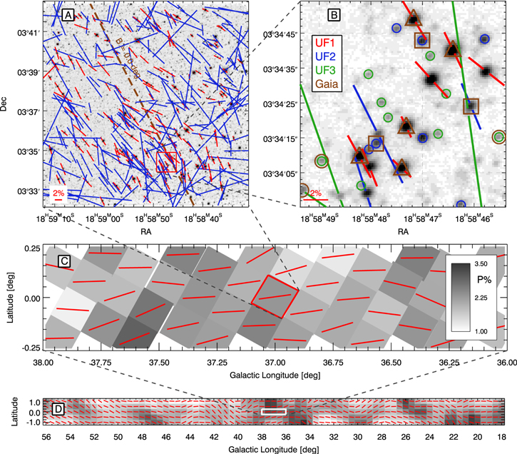
Figure 1. Multiscale overview of GPIPS data products and derived quantities. (Upper left, panel A): equatorial, reversed gray-scale representation of the deep photometric image for field number 1619. Colored lines through stars encode UF1 and UF2 P' and EPA. UF3 information is suppressed in this panel. A red 2% P' reference scale appears in the lower-left corner. The Galactic equator is identified by the brown, dashed, diagonal line and the "B = 00" label. (Upper right, panel B): enlargement of selected portion of panel A. Colored lines identify polarization detections and circles identify P' upper limits. Gaia DR2 star matches are shown as the brown symbols. (Middle, panel C): a 2 × 05 portion of the northern Galactic midplane, shown in Galactic coordinates. Individual GPIPS FOVs are shown as rotated gray squares, aligned to Galactic orientations. Gray-scale shade encodes median percentage polarization, ranging from 1% (white) to 3.5% (black). Red lines (of uniform length) represent the median Galactic polarization position angle of the UF1 stars in each FOV. They reveal a mostly disk-parallel magnetic field, but also some departures from uniformity. (Bottom, panel D): low-resolution representation of the median polarization percentage and median polarization position angles across the full GPIPS survey region. The gray scale encodes median polarization percentage, from 1.1% (white) to 2.4% (black).
Download figure:
Standard image High-resolution imageIn Figure 1, upper right, panel B, shows a zoomed-in view of a 60 × 60 arcsec2 region drawn from the upper left, panel A. In panel B, the inverse gray-scale shows the presence of many tens of stars. The mean PSF FWHM is 18, which is only somewhat greater than the average for the entire GPIPS data set. Lines and circles indicate stellar polarization detections (P' > 0%) and upper limits (P' = 0%), respectively: red for UF1 stars (eight detections, no upper limits), blue for UF2 stars (three detections, seven upper limits), and green for UF3 stars (three detections, eight upper limits). Orientation line lengths encode debiased linear polarization percentage in H band. Line orientations encode polarization equatorial position angles. Nearly all of the stars in panel B have been measured for polarization, as noted by their hosting either an associated orientation line or a circle.
In panel B, Gaia DR2 stars are indicated as brown symbols. All stars that appear in Gaia DR2 are matched to POLCAT entries for this 1 × 1 arcmin2 field. Yet, the natures of the Gaia-matched stars are complex. Only five of the eight UF1 stars have Gaia matches, with a couple of the most NIR-bright UF1 stars not matched to Gaia stars. These nonmatches are strongly reddened (mean H − K ∼ 1.2 mag, or AV ∼ 17 mag), which affects Gaia g-band, optical magnitudes more than GPIPS H-band magnitudes. The effects of reddening on the ability of Gaia to provide distances to GPIPS POLCAT stars are explored in greater detail in Section 4.1.
The middle, panel C, of Figure 1 spans 2° of Galactic longitude and presents each plotted GPIPS FOV as a single, gray-scale, rotated square with an inset red orientation line. The rotation of the field from panel A to panel C is due to the relative orientations of the equatorial orientation of Mimir and the Galactic plane. Each of the 41 FOVs shown in panel C is shaded to represent a single representative polarization percentage. These were computed as the medians of the UF1 star values for each FOV and are encoded as gray-scale values, where black represents the greatest polarization percentage. A single red orientation line is oriented in each FOV to display the similarly computed mean polarization position angle, in Galactic coordinates.
These representative values were obtained from the median values of the polarization percentage and Galactic position angle (GPA) for the UF1 stars in each FOV, as described in Section 4. They represent a single, coarse characterization of the polarization properties for each FOV. Across panel C, the mean H-band polarization fraction is seen to vary from a low of 1% to a high of 3%, with the panel-A field exhibiting a value of 2.3%. The red lines show that the magnetic field being traced (at 10' resolution) is mostly parallel to the Galactic plane, but some FOVs also exhibit significant, coherent deviations of polarization position angle.
The bottom, panel D, of Figure 1 encompasses the entire GPIPS region with representations of polarization percentage and position angle that relate to those shown in the previous panels. The single-FOV median properties of P' and GPA of the UF1 stars were smoothed, using Gaussian distance weighting (FWHM = 075) onto a 0.5 × 0.5 deg2 grid. The red position angle orientation lines are mostly parallel to the Galactic plane, but again show significant deviations, notably near Galactic longitudes 22°, 29°, 34°, 41°, 44°, and 52°–56°. The averages shown are coarse representations, as no Stokes U, Q averaging was performed—instead, straight averages of the FOV median values were used.
GPIPS data reveal a generally disk-parallel magnetic field, with some departures likely due to interactions with the gas dynamics present in the thin, molecular disk of the Milky Way.
4. Analyses
This section begins with an analysis of the natures of the GPIPS stars that match, and do not match, to Gaia DR2 stars. The details of the matching algorithm and the resulting match statistics may be found in Appendix B. In Section 4.2, characterizations of the data products from the same central FOV of the GPIPS survey (number 1619; Figure 1(A)) are described and evaluated to introduce the FOV-based stellar polarization characterizations employed throughout the subsequent analyses. These single-FOV evaluations provide physical insight into the nature of the region being probed and the magnetic field properties sampled along the sight lines contained in each FOV. These characterizations were then applied to the entire set of GPIPS FOVs, as described in Section 4.3, to establish general distribution functions (i.e., marginalized over GL and GB, so zero dimensional), one-dimensional (1D) Galactic longitude and latitude distributions of the polarization properties, tests for correlations among the properties, and two-dimensional Galactic directional distributions of the polarization properties.
4.1. The Natures of the GPIPS-to-Gaia Matching, and Nonmatching, Stars
The utility of GPIPS data products for revealing magnetic field properties depends on the characteristics of the stars observed, as well as the natures of the dust and gas distributed along the lines of sight to the stars. The GPIPS observations were designed (Paper I) to ensure that most of the stars that would have polarization detections would be moderately extincted (1 ≤ AV ≤ 30 mag), and thereby polarized, distant giants. The analysis of the first 17% of GPIPS data (DR1; Paper III) confirmed the expected excess of giants over nearby dwarfs. Stellar reddening excesses  as great as 2 mag were found in DR1. Such excesses implied that extinctions were being probed to about 30 mag of AV.
However, accurate distances to the GPIPS stars remained elusive until the release of Gaia DR2. One important distance to establish is the minimum needed through the diffuse ISM to develop detectable NIR polarization signatures to GPIPS levels. This "near horizon" for GPIPS is likely beyond the extent of the Local Bubble (Lallement et al. 2003), but is it close enough to reveal magnetic fields for dark molecular clouds at 300–400 pc? The "far horizon" would be the distance limit beyond which GPIPS stars are too faint or too extincted to be detected. Both distances are needed to estimate the range of line-of-sight distances over which GPIPS data offer the most useful magnetic field information.
The matching of Gaia and GPIPS stars, described in Appendix B, led to the creation of FOV-based files of Gaia star information and their corresponding GPIPS star match identifiers. Examination of the characteristics of the stars with GPIPS–Gaia matches, and those without such matches, was performed to establish stellar characterizations and to reveal the GPIPS near and far horizons.
Figure 2 displays contour representations of the stellar count density distributions of selected Gaia stars matched to subsets of GPIPS stars, as functions of the optical, g-band (Gaia Collaboration et al. 2018b) apparent magnitude and the base 10 log of the Gaia parallax π (in mas) to each star. Gaia stars included in this plot had g-band magnitude uncertainties less than 0.66 mag, parallax S/Ns (≡π/σπ) ≥ 0.5, and parallaxes π > −2 mas. These liberal limits were chosen to avoid introducing parallax bias (Bailer-Jones et al. 2018; Luri et al. 2018) to the sample population characteristics. These criteria selected for just over 40% of all Gaia stars appearing in the GPIPS FOVs.
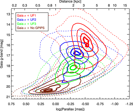
Figure 2. Comparison of Gaia g-band apparent magnitudes vs. Gaia parallax for stars matched and not matched to GPIPS POLCAT entries. Bottom horizontal axis presents base 10 logarithm of the parallax in milliarcseconds. Upper horizontal axis shows corresponding distances. Densities of star counts in this plane are indicated by the colored contours, with values of 10% and 25% (dashed lines) and 50%, 75%, 90%, and 97.5% (solid lines) of the peak value for each of the four subsamples of stars. Red contours show the distribution of Gaia stars that match to UF1 stars in POLCATs. Blue contours represent Gaia stars matched to UF2 stars, and green contours represent UF3 stars. The brown contours show the distribution of Gaia stars with parallaxes that have no matching stellar entries in the GPIPS POLCATs. The POLCAT-matching stars tend to be brighter and more distant than the nonmatching stars.
Download figure:
Standard image High-resolution imageIn Figure 2, contours shown in red represent the stellar count density of the selected Gaia stars in the magnitude–parallax plane that matched to POLCAT UF1 stars ("Gaia π + UF1" in the legend). These matched stars account for only 3.4% of all Gaia stars but 46% of all POLCAT UF1 stars. The portion of the figure exhibiting 50% of the peak density of counts of Gaia parallax stars ("Gaia π" hereafter) matched to UF1 stars (marked by the outermost solid red contour) spans g-band apparent magnitudes of about 14th–18th and log parallaxes of −0.26 to −0.85, or distances of 1.8–7.1 kpc.
The blue contours in Figure 2 represent the density of counts of Gaia π stars matched to POLCAT UF2 stars, and the green contours represent the same for UF3 stars. They both span correspondingly fainter apparent magnitudes at somewhat closer distances than do the UF1 stars (red contours). Ignoring extinction (but see the discussion regarding Figure 4 below), the g-band absolute magnitudes of the peaks of the UF1 (red), UF2 (blue), and UF3 (green) distributions, after correcting for the distance moduli implied in the parallaxes, are about 3.1, 5.0, and 6.7 mag at inferred mean distances of about 3.2, 2.3, and 2.0 kpc, respectively. (These and other values are collected in Table 2).
Table 2. Summary of UF Sample Stellar Distributions Properties
| Sample | ||||
|---|---|---|---|---|
| Property | UF1 | UF2 | UF3 | Gaia, No POLCAT |
| (1) | (2) | (3) | (4) | |
| Figure 2 based: Locations of distribution peaks, no AV corrections applied | ||||
| mg (mag) | 15.6 | 16.8 | 18.2 | 20.4 |
| log π (mas) | −0.50 | −0.36 | −0.30 | +0.11 |
| Distance (kpc) | 3.2 | 2.3 | 2.0 | 0.78 |
| Mg (mag) | 3.1 | 5.0 | 6.7 | 10.9 |
| Figure 3 based: Sample fractions of GPIPS POLCAT stars | ||||
| No 2MASS (σ(H − K) > 0.5 mag) (%) | 8.2 | 27.3 | 69.4 | ... |
| No Gaia Match (%) | 14.0 | 24.2 | 17.5 | ... |
| Gaia Match, no π (%) | 31.9 | 22.5 | 5.4 | ... |
| Gaia Match, π (%) | 45.9 | 26.0 | 7.6 | ... |
| Figure 4 based: Distribution properties for Gaia π subsamples | ||||
| Distance, in kpc, to cumulative percentage of subsample: | ||||
| 0.5% | 0.35 | 0.35 | 0.33 | ... |
| 10% | 0.91 | 0.72 | 0.71 | ... |
| 50% | 2.63 | 1.95 | 1.78 | ... |
| 90% | 6.17 | 4.90 | 4.22 | ... |
| 99.5% | 11.89 | 10.59 | 9.44 | ... |
| Av at distrib. peak (mag) | 3.2 | 1.6 | 2.2 | ∼0 |
| Derived properties, with AV corrections applied | ||||
| Mg (mag) | −0.1 | 3.4 | 4.5 | ∼11 |
| Gaia colors (GBP–GRP) (mag) and approx. spectral types | ||||
| Lum. Class III | +1.04 to +1.46 | +1.07 to +1.20 | ... | ... |
| G7–K2.5 III | G7–K0 III | ... | ... | |
| Lum. Class V | −0.04 to +0.19 | +0.63 to +0.98 | +0.74 to +0.96 | +2.63 to +2.91 |
| A2–A7 V | F4–G8 V | F8–G7 V | M1.5–M3 V | |
| Lum. Class VII | ... | ... | ... | −0.27 to −0.11 |
| ... | ... | ... | DA(?)VII | |
Download table as: ASCIITypeset image
The brown contours in Figure 2 indicate the density of Gaia stars that meet the magnitude and parallax S/N selection criteria but for which no POLCAT star was matched. Again, ignoring extinction, the g-band absolute magnitude for the peak of this distribution is about 10.9 mag, at a distance of about 0.78 kpc. Hence, the Gaia π stars that match to POLCAT entries have brighter g-band apparent magnitudes and are at greater distances, and are thereby more luminous, than the Gaia π stars that do not match to POLCAT entries.
Establishing characteristic distances to the GPIPS stars (the near and far horizons) requires correcting the Gaia distances for the effects of dust extinction. This affects the optical, g-band magnitudes of Gaia more than it affects the NIR magnitudes of GPIPS. In Figure 3, contours of star counts in the (H − K) versus H-band color–magnitude plane have been color-coded to identify nine selected subsets of stars. Stars in POLCATs that had Gaia π matches are represented by the red, blue, and green contour distributions, based on their UF1, UF2, or UF3 designations, as was done in Figure 2. Stars in POLCATs with Gaia star matches that did not meet the parallax criteria ("Gaia no π"), are represented by the orange, purple, and cyan colored contour distributions, based on their UF1, 2, and 3 designations, respectively. GPIPS stars that did not match to any Gaia stars are shown by the yellow, magenta, and dark-green contours. All POLCAT NIR stellar magnitudes and colors included in the distributions were drawn from 2MASS (Skrutskie et al. 2006), subject to a (H − K) color uncertainty criterion of ≤0.5 mag. These 2MASS and Gaia selection criteria, taken together, tend to bias the distributions against faint and red stars. This is seen as the successively smaller fractions of the total POLCAT stars with increasing UF number in Table 2.
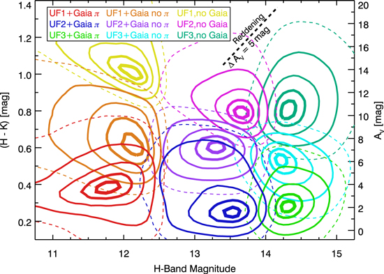
Figure 3. Comparison of 2MASS H-band magnitudes and (H − K) colors for matching GPIPS UF1 (mH ∼ 12), UF2 (mH ∼ 13–14), and UF3 (mH ∼ 14–15) stars. A scale for visual extinction, assuming average dust properties, is shown as the right axis. A reddening vector, corresponding to an AV change of 5 mag, is shown in black on the upper right. At each UF designation, three vertically offset colored sets of contours show subsets of stars for that designation that have different Gaia DR2 matching properties. A legend relating contour set color to Gaia DR2 matching properties is shown on the upper left. The lowest contour sets (red, blue, and light green), centered at the least red (H − K) (least AV) values, represent star count densities of GPIPS stars matching Gaia stars that have good parallax values (e.g., "UF1+Gaia π" in red in the legend). The middle contour sets (orange, purple, and cyan) represent GPIPS stars that match to Gaia stars, but for which there are no good parallax values. The highest contour sets (yellow, magenta, dark green) represent GPIPS stars that do not match to Gaia stars. All contour sets are drawn representing 25% (dashed) and 50%, 75%, 90%, and 97.5% (solid) of the peak stellar counts in each distribution.
Download figure:
Standard image High-resolution imageThe groupings in Figure 3 reveal the expected magnitude boundaries separating UF1, 2, and 3 stars. These boundaries are seen as the node-like vertical contours near mH = 12.5 and 14 mag, which are manifestations of the imposed UF definitions. The right axis indicates approximate values of AV, from 0 to 20 mag, using the NIR Color Excess method (NICE; Lada et al. 1994).
GPIPS stars with Gaia π matches tend to be less extincted than GPIPS stars of similar H-band brightnesses, but for which the Gaia matches yielded no parallaxes. The GPIPS stars not matching to Gaia stars are the most extincted of all, as already noted in the Figure 1(B) discussion. For the POLCAT stars matched to Gaia π stars (the red, blue, and green contours), the UF1 distribution peak exhibits AV about 2 mag greater than seen at the UF2 and UF3 peaks. The UF2+Gaia π distribution shows a bifurcation in AV, with components near 2 and 6 AV mag. The POLCAT stars matched to Gaia no π stars show distribution peaks offset from the Gaia π stars distribution peaks by 3.5, 5.5, and 4.0 AV mag for UF1, 2, and 3, respectively. The POLCAT stars not matched to Gaia stars show distribution peaks offset from the Gaia π stars distribution peaks by 10, 8.5, and 8.5 AV mag, respectively. The AV steps within each UF vertical group, of about 4 mag for Gaia π to Gaia no π and another 4 mag to the no-Gaia stars, show that Gaia selects the lowest extinctions while GPIPS without Gaia stars selects the most extincted stars.
The UF1 stars with Gaia π matches represent 45.9% of all UF1 stars (FOV-based). The unmatched and no parallax subsets contain 14.0% and 31.9% of all UF1 stars, respectively. The remaining 8.2% of UF1 stars fails to meet the 2MASS color uncertainty criterion applied. Moving to the fainter, UF2 stars, those with Gaia matches and parallaxes account for 26.0% of all UF2 stars (FOV based), the Gaia-unmatched and no parallax subsets account for 24.2% and 22.5%, respectively, and the remaining 27.3% fails the color uncertainty selection criterion. The faintest, UF3, stars with Gaia matches and parallaxes account for only 7.6% of UF3 stars, while only another 17.5% and 5.4% are in the Gaia-unmatched and no parallax subsets. The high fraction of UF3 stars failing the 2MASS color uncertainty selection criterion, 69.4%, is because GPIPS probed stars fainter and/or redder than stars in the 2MASS catalog.
In Figure 4, extinctions and parallaxes for Gaia π stars matched to POLCAT entries are represented as the red-, blue-, and green-colored contours of stellar density for UF1-, UF2-, and UF3-matched stars, respectively, in the central panel A . The stars contributing to Figure 4 were required to have the same (H − K) color uncertainty ≤0.5 mag, parallax S/N ≥ 0.5, and parallax greater than −2 mas as for the previous figure. POLCAT stars matched to Gaia π stars tend to have extinctions ranging from 0 to >6 mag of AV, and span distances of <0.5 to about 15 kpc. The distances corresponding to the locations of peaks in the contour distributions are similar to those described for Figure 2, for each of the three subsets of stars.
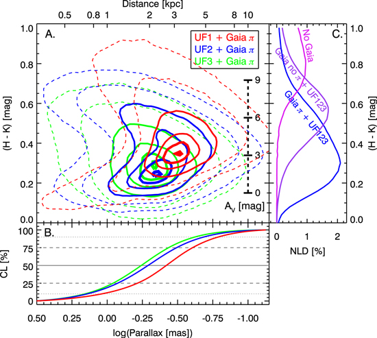
Figure 4. Comparison of 2MASS (H − K) colors with Gaia parallaxes for DR4 POLCAT stars. (Central, panel A): contours of normalized star count density for Gaia stars with parallaxes matched to POLCAT stars. Contours represent 10% and 25% (dashed) and 50%, 75%, 90%, and 99% (solid) of the peak star count density in each sample. Extinction scale is shown inset at right; distance scale is shown along the top axis. (Bottom, panel B): cumulative likelihood (CL) for the Gaia π-matching POLCAT stars. Gray dotted, dashed, and solid lines are drawn at 10%, 25%, 50%, 75%, and 90% cumulative probabilities. (Right, panel C): normalized likelihood distributions (NLD) histograms of (H − K) colors for POLCAT stars matched to Gaia π stars (blue curve), POLCAT stars matched to Gaia no π stars (purple), and POLCAT stars not matched to Gaia stars (magenta). The POLCAT stars without Gaia matches tend to exhibit greater values of extinction than the stars with Gaia matches.
Download figure:
Standard image High-resolution imageThe lower panel B of Figure 4 shows the marginalization over NIR color as cumulative likelihoods (CL) of star count density with log parallax for each of the UF1, UF2, and UF3 samples that match to Gaia π stars and also satisfy the selection criteria applied to the 2MASS values. The UF1 CL (red) curve crosses the 10% and 90% horizontal dotted gray lines at about 0.91 kpc and 6.3 kpc, respectively. That CL curve also shows quartile boundaries at 1.6, 2.63, and 4.1 kpc. The UF2 CL (blue) curve shows a median of about 1.95 kpc, with 10% and 90% limits of 0.72 and 4.0 kpc. UF3 stars (green CL curve) have a median distance of 1.78 kpc, with 10% and 90% limits of 0.71 and 4.22 kpc. The 2MASS selection criterion on color uncertainty added some bias against fainter stars, so the distance values quoted here should be considered upper and lower limits, respectively, for the 10% and 90% values, though they are reasonably characteristic of the samples.
In the right panel C of Figure 4, the central panel distributions have been marginalized over the parallax to create histograms of (H − K) colors of stars in the Gaia π, Gaia no π, and no-Gaia groups, shown as the blue, purple, and magenta curves, respectively. The histograms have been normalized by the sum of the stars contained in the 0.02 mag wide bins in both histograms. These histograms reveal similar extinction offsets between the ∼1.6 million Gaia π matched, the ∼1.1 million Gaia no π matched, and the 0.6 million Gaia-unmatched samples of about 4.5 mag of AV between each successive group, similar to what was seen in Figure 3.
The more distant UF1 stars with Gaia π matches were also found to be somewhat more extincted than the fainter UF2 and UF3 subsets, at least for the contours near the peak regions of the star count distributions. As shown in panel C of Figure 4, the stars without Gaia matches are even more extincted, on average, than the Gaia π- and Gaia no π-matched UF1 stars. Correcting for the extinctions corresponding to the peaks of the colored contour distributions in Figure 4(A) (see Table 2), the g-band apparent magnitudes found in Figure 2 become g-band absolute magnitudes Mg of about −0.1, 3.4, and 4.5 mag, for the UF1, UF2, and UF3 samples, respectively.
Table 2 provides a summary of key characteristics of the different samples of stars analyzed in this section. The columns identify the UF designation of the sample, or for the case of Gaia stars that do not match to POLCAT stars, a "Gaia, No POLCAT" column. The rows list the source of the properties in the preceding text, mostly derived from the Figures 2–4 plots of the two-dimensional distributions of stars that match among the POLCATs, Gaia, and 2MASS. The locations of the peak stellar densities in Figure 2 are listed but have not been corrected for extinction effects. In Figure 3–based rows, the UF1+Gaia π subsample is seen to account for about 46% of all UF1 stars, while the fainter UF2 and UF3 stars are less well represented by matches to the 2MASS and Gaia π archival catalog data and so the propertied derived might not be as accurately characterized for these stars. In the Figure 4–based rows, the Gaia π match subset estimates for the near, far, and mean distances for each sample are listed for multiple population percentage steps in the cumulative probability distributions.
To estimate the spectral types of the POLCAT stars, the Gaia H-R diagram for low-extinction stars presented as Figure 5 in Gaia Collaboration et al. (2018a) was employed. For each of the AV-corrected Mg values noted above, the range of Gaia colors (GBP–GRP) spanned by the majority of stars was identified for the three main luminosity classes (III, V, VII) and these values are reported near the bottom of Table 2. These colors were converted to Johnson−Cousins (V − I) using the analysis of Gaia colors reported in Evans et al. (2018). The (V − I) colors were used to retrieve spectral types for the associated luminosity classes using the tables published in Ducati et al. (2001), except the white dwarfs. In the absence of characterizing spectra, these were assigned DA(?) types.
These spectral-type ranges are based on the g-band apparent magnitudes, Gaia parallaxes, 2MASS colors, and standard NICE conversions to AV drawn from values at the peaks of each distribution in Figures 2–4. The contoured distributions shown in these figures also span ranges of all those quantities, so the derived spectral types should be viewed as notional characterizations, not quantitatively limited ones.
In Table 2, the UF1+Gaia π matched stars span spectral types of G7–K2.5 in the giant luminosity class and A2–A7 in the dwarf class. However, the former is more likely to represent the stars in the UF1 subset, as A-type stars are rare in Figure 5 of Gaia Collaboration et al. (2018a), whereas that giant range takes in much of the highly populated Red Clump (e.g., Pavel 2014). For the UF2 stars, both giant and dwarf branches are likely, with a slight dominance by the dwarfs. This luminosity class bifurcation might be a partial cause of the AV bifurcation of the UF2+Gaia π distribution (blue contours) in Figure 3. The UF3 stars show a distribution of peak Mg values that only slice through the dwarf sequence of Figure 5 in Gaia Collaboration et al. (2018a) and only do so for spectral types somewhat later than those of UF2 and quite distinct from the ones for UF1.
The Gaia stars not matched to POLCAT stars were already shown to be much closer than the UF1, 2, or 3 stars. Given the proximity of these Gaia-only stars, extinctions are likely much less than one magnitude of AV. As such, their inferred Mg values slice through both the white dwarf and dwarf sequences in Figure 5 of Gaia Collaboration et al. (2018a). Given the high space density of red dwarf stars, it is likely they dominate this POLCAT-unmatched subset of stars.
It is more difficult to assign distances and spectral types to POLCAT stars in the no-Gaia and Gaia no π subsamples. Figure 3 includes a reddening line that can aid in interpreting the nature of the stars in these subsamples. For example, the slope of the reddening line is such that the UF1+Gaia no π (orange contours) subset could be deextincted by about 4 AV mag to fall closely over the UF1+Gaia π (red) subset. If this is the case, then both subsets would have nearly identical spectral types and distances, with the Gaia no π subset merely suffering additional extinction, likely associated with denser molecular cloud directions. Interestingly, the UF1 no-Gaia (yellow contours) subset, if deextincted by 10 mag to the UF1+Gaia π value of about 4 AV mag, would have brighter apparent magnitudes than the UF1+Gaia π subsample. This could be caused by the UF1 no-Gaia stars being closer or by having greater luminosities, perhaps caused by supergiants located at much greater distances. The very red (H − K) colors for the UF1, no Gaia stars, of 1.0 mag and beyond, cannot be due to nearby red dwarfs, however, as shown in the relative color–color diagram of Figure 19 in Paper III. Simulations of stellar types, distance, and extinctions with GPIPS and Gaia detection limits imposed as priors are beyond this present treatment. Yet, it does appear likely that all of the UF1 stars, across all Gaia-based subsets, are similar enough as to be recognized as red giants, many in the Red Clump, with various degrees of foreground reddening and extinction. The extinctions could be associated with individual dark clouds, with spiral arms that lie between 1 and 7 kpc such as Sagittarius and Scutum, or even with the central Galactic Bar.
Figures 2–4, taken together, provide the information necessary for identifying the near- and far-side GPIPS "horizons." As listed in Table 2, 99% of UF1 stars are located between distances of 0.35 and 11.9 kpc, with 90% between 0.63 and 7.5 kpc. Thus, there are sufficient UF1 and UF2 stars to conduct limited angular resolution polarization probes of molecular clouds as close as 350–400 pc as well as to characterize magnetic fields in spiral arms in the Galactic midplane.
Having established the bases and representative values for the GPIPS horizons, an exploration of the NIR GPIPS linear polarization properties for one FOV is described in the following.
4.2. Methods and Characterizations for One Field, GPIPS-1619
The data from the GPIPS-1619 field, shown in Figure 1(A), were used to explore methods of analyzing and characterizing the polarization properties of the stars for one FOV. This began with plots of basic data properties and proceeded to analyses of distributions of those properties.
Figure 5 displays, for the stars in the GPIPS-1619 FOV, the dependence of polarization position angle relative to the Galactic frame of reference (GPA) on the stellar H-band magnitude (upper left, panel A) and on debiased polarization percentage (upper center, panel C). The 197 UF1, 557 UF2, and 1172 UF3 stars in the POLCAT for GP1619 were trimmed to remove polarization upper limits (σP ≥ PRAW), as they contribute no meaningful GPA values. The remaining 179 UF1, 352 UF2, and 563 UF3 stars are plotted as the red, blue, and green symbols, respectively. The 129 member subset of UF1 stars that exhibit P'S/N (P'/σP) ≥ 3 (equivalent to σPA < 96), and designated UF0, are plotted as filled light-brown squares, which appear within most of the red UF1 star location circles.
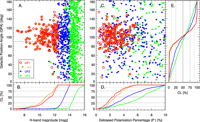
Figure 5. Polarization position angle in Galactic coordinates (GPA) vs. H-band stellar magnitude (left, top, panel A) and vs. debiased polarization percentage P' (center, top, panel C) for GPIPS FOV number 1619. Symbol colors identify stellar classification by UF number, as shown in the legend in the lower-left corner of panel A. The dashed horizontal gray lines at 90° in panels A and C indicate the Milky Way disk-parallel GPA value. The brighter, UF1 stars (red open circles), most of which are also members of the UF0 subset (light-brown filled squares), exhibit lower polarization percentages and a smaller spread in GPA values, compared to the moderately fainter UF2 (blue) and much fainter UF3 (green) stars, though the non-UF1 stars retain some information concerning the B fields they trace. Panels B, D, and E present cumulative likelihood (CL) distributions, after marginalizing over the other dimension, for each UF stellar subset. Panel B (left, bottom) reveals median H-band magnitudes of 10.8, 11.5, 13.3, and 14.6 for the UF0, UF1, UF2, and UF3 subsets. Panel D (center, bottom) CL distributions do not include polarization upper limits or P' values in excess of 10%. The UF2 and UF3 distributions are shifted to higher P' values due to bias from their uncertainty contributions. Panel E (rightmost) shows CL distributions with a strong concentration near 100° (UF0, UF1) or much weaker concentrations closer to 90° (UF2, UF3).
Download figure:
Standard image High-resolution imageThe UF1 (and UF0) stars, and many UF2 stars, exhibit GPA values in the 70°–130° range (panel A) and P' values in the 0.5%–5% range (panel C). The UF2 stars tend to exhibit higher P' values than do the UF1 stars, and this tendency is even stronger for the fainter, UF3 stars. Some of these higher polarization percentages could be real and could correlate with higher dust column densities and coherent magnetic field orientations, traceable through extinction. However, these fainter stars are more likely to exhibit higher P' values due to noise bias and those values should be treated with caution (Paper III). Lower limits on P'S/N alone are not sufficient to select high-confidence stellar polarizations, unless the limit values are quite high (e.g., greater than 3–5; Simmons & Steward 1985).
In Figure 5, the upper-left panel A exhibits the expected delineations into the UF designations of stars as a function of H-band magnitude. These boundaries are sharpest at the faint limits of UF1 (mH = 12.5 mag) and UF2 (mH = 14 mag). However, because the UF definitions are based on both magnitude and polarization uncertainty, the minority presence of some UF2 and UF3 stars across the magnitude boundaries is to be expected. The main conclusion from the distribution of stars in panel A is that the UF1 (and UF0 subset) stars appear near, but not completely on, the GPA = 90° disk-parallel line. The UF2 stars have a similar though much weaker correlation with the same orientation, and the UF3 stars are only weakly constrained in their GPA values.
In Figure 5, panels B, D, and E present cumulative likelihoods of the marginalized distributions, color-coded by UF designation in the same fashion as for the plotted symbols in panels A and C. Panel B (lower left) shows how the UF subsets are distributed with H-band magnitude. Median magnitudes are 10.8, 11.5, 13.3, and 14.6 mag for the UF0, UF1, UF2, and UF3 samples, respectively. Panel D (center-bottom) shows the CL curves of P' after being marginalized over GPA. However, the likelihood accumulation window was truncated at 10% of P', which affects the UF2 and UF3 CLs, as some of those stars have P' values in excess of that limit. In that panel D , the P' medians of 2.4% and 2.7% for UF1 and UF0 are accurate, but the UF2 and UF3 medians of 4.4% and 6.5% represent only lower limits because of the truncation.
The GPA CLs, marginalized over  , but including the truncation at 10%, are shown in panel E (rightmost) of Figure 5. The medians for UF0 and UF1 are both 102°, while UF2 shows 98° and UF3 shows 94°. The UF0 and UF1 CL curves show the least separations between their first and third quartiles at 25°, UF2 is intermediate at 52°, while UF3 is the widest at 80°, a value close to the 90° expected for a random distribution.
The GPA distributions of Figure 5 were used to compute a mean value of GPA and its standard deviation (ΔGPA) for each UF subset of stars. These values were computed both in an unweighted fashion, without respect to individual GPA uncertainties, and using variance weighting by those uncertainties. (Note that Stokes U and Q averaging was not performed—the analyses used GPA values only.) The resulting values appear in Table 3. The first column in the table indicates the UF star subset, with UF0 entries shown in italics to highlight that it is a subset of UF1. The numbers of GPIPS-1619 stars with detected debiased polarizations used in each UF sample is in the second column. The remaining columns list the unweighted GPA means, the unweighted GPA standard deviations, the weighted GPA means (with propagated uncertainties in parentheses), and the weighted GPA standard deviations (and uncertainties).
Table 3. GPIPS-1619 Average Galactic Position Angles
| UF | Num. | Unweighted | Weighted | ||
|---|---|---|---|---|---|
| Subset | P' > 0% |

|
ΔGPA |

|
ΔGPA |
| (deg) | (deg) | (deg) | (deg) | ||
| (1) | (2) | (3) | (4) | (5) | (6) |
| UF1 | 179 | 100.8 | 16.1 | 102.88 (0.32) | 14.69 (0.32) |
| UF0 | 129 | 101.4 | 15.9 | 102.94 (0.33) | 14.62 (0.33) |
| UF2 | 352 | 95.2 | 39.7 | 97.5 (1.0) | 40.6 (1.0) |
| UF3 | 563 | 90.9 | 50.2 | 88.5 (0.9) | 51.3 (0.9) |
Download table as: ASCIITypeset image
The UF1 (and UF0) stars show the greatest mean GPA departure from the disk-parallel value of 90°, while the UF3 stars show the least such departure. The standard deviation progression with UF type is stronger, with the UF1 (and UF0) stars having a weighted ΔGPA of under 15°. The UF2 and UF3 samples, with ΔGPA values of 41° and 51°, respectively, are close to being completely uniform in their GPA spreads (for which ΔGPA would be 52°). There are no major differences in mean GPA or ΔGPA between the unweighted and weighted values, though the latter provide uncertainties that give context to the values.
4.2.1. Analyses Based on UF1 Stars
Characterizing the properties of the Galactic disk magnetic field using GPIPS data products can proceed along many different paths, invoking a wide variety of data selection criteria. This could include, for example, utilizing all of the GPIPS stellar Stokes U and Q measurements, or alternatively, selecting only the data corresponding to high P'S/N (e.g., ≥5). All choices of data selection schemes bring some type of bias, or focus, on a particular data range or ISM characteristic. High P'S/N cutoffs select the highest-quality polarization measurements, but reduce the number and spatial sampling that could reveal magnetic field properties with adequate confidence levels. Low P'S/N cutoffs introduce excessive noise and false positives. In Appendix C, the UF1 stellar subset is shown to reveal similar properties to those found in the high-P'S/N UF0 subset. This reduces the need to restrict further analyses to the smaller UF0 subset, as the larger UF1 set is adequate for establishing overall magnetic field properties and correlations. The UF1 stars suffer less noise-biasing effects than fainter stars and thus enable higher-significance differential comparisons of polarization properties between GPIPS FOVs than would be possible using UF2 and/or UF3 stars.
For those reasons, the analyses presented in the remainder of this section and in all of the following sections were performed by focusing on the properties of the stars classified as UF1 in each of the 3237 GPIPS FOVs. Future studies utilizing other subsets of the GPIPS stars, with other selection criteria and with different weighting schemes, could reveal additional magnetic field behavior that may be missed in the current analyses. Indeed, Bayesian analyses (e.g., Clemens et al. 2018) have already shown great promise for combining a wide range of P'S/N stellar polarization values with Gaia distance information.
4.2.2. Polarization Properties of the UF1 Stars
Figure 6 shows histograms of the debiased polarization percentage P' (left, panel A) and GPA (right, panel B) for the 179 UF1 stars that have P' > 0% in the GPIPS-1619 FOV. These histograms were constructed in a manner designed to account for the uncertainties in the individual measured P' and GPA values via accumulation of representative Gaussian probability distributions (described in the Appendix of Clemens et al. 2013). This process results in smoother histograms than if the P' and GPA values were directly binned and more accurately reflects the likelihood functions for these quantities. The P' histogram (panel A) peaks at just under 2%, and the GPA histogram7 is centered near 100°.
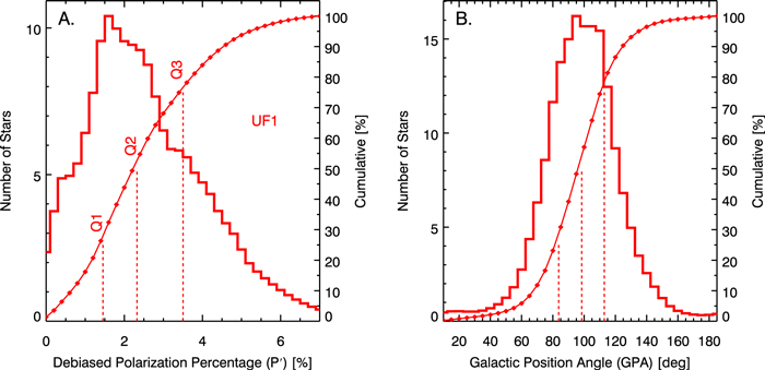
Figure 6. Histograms of debiased polarization percentage P' (left, panel A) and Galactic position angle GPA (right, panel B) for UF1 stars in GPIPS-1619. The histograms were constructed using accumulated Gaussian distribution representations for the properties of each star, as noted in the text. Cumulative probability distributions are shown as the smooth curves that connect points centered in each bin and are referenced to the right axis labels. Vertical red dashed lines and labels identify the locations of the three quartile boundaries of the cumulative distributions.
Download figure:
Standard image High-resolution imageAcross the full set of GPIPS FOVs, many of the resulting histogram probability functions were asymmetric and sometimes double peaked. Hence, simple representative functions or fits, such as Gaussians, cannot accurately characterize the actual distributions.
Accordingly, cumulative probability distributions were computed for the UF1 subset for each histogram and are overlaid as thin red lines in Figure 6. These were analyzed to find the quartile boundaries (Q1 = 25%, Q2 = median, and Q3 = 75% cumulative probability). The resulting median P' (hereafter P50) for this field is 2.32%, while the median GPA (hereafter GPA50) is 985. The combination of GPA50 in Figure 6(B) being 985 for UF1 stars while the weighted mean for the same stars in Table 3 is 1029 ± 03 is evidence that the Figure 6(B) UF1 distribution has some non-Gaussian nature, despite its Gaussian appearance. The values for the first and third UF1 quartile boundaries are 1.45% and 3.50% for P' and 837 and 1129 for GPA, as indicated on Figure 6.
In order to obtain robust measures of the widths of the GPA distributions, the interquartile ranges, computed from the differences between the x-axis locations of the first and third quartiles (Q3–Q1), were adopted. For the GPIPS-1619 GPA histogram, this width difference, designated WGPA, is 292 for the UF1 stars. If the GPA distributions were perfectly Gaussian, the Gaussian width parameters would be 42.5% of the WGPA values, or about 124 for the GPIPS-1619 FOV. This value is somewhat less than the standard deviations reported in Table 3, again indicating that some non-Gaussian nature characterizes the GPIPS-1619 UF1 GPA values.
Similar histogram analyses were performed using the UF1 stars contained in the POLCATs for each of the GPIPS FOVs. The four key characterizing values extracted for each FOV included the numbers of UF1 stars in each field, their median P' values (P50), their median GPA (GPA50), and their interquartile range of the GPA histograms (WGPA), all of which are evaluated in the following.
4.3. FOV-based GPIPS Characterization of Polarization and Magnetic Field Properties
In this section, histograms of these four key characterizing quantities are presented, as are their distributions as functions of Galactic longitude and latitude, at the 10' angular resolution corresponding to the Mimir FOV size. This selection enables the generation of high-significance values by quantifying the behavior of the properties of the many UF1 stars in each FOV; doing so reveals both large-scale trends and moderate-scale departures from those trends. Detailed examination of properties on finer angular scales and across overlapping FOVs is needed, for example, to establish the magnetic field properties associated with resolved molecular clouds (e.g., Marchwinski et al. 2012; Hoq et al. 2017), but is beyond the scope of this paper.
The large-scale, FOV-based characterizations begin with histogram analyses of the numbers of UF1 stars measured for polarization in each FOV, the median polarizations, the median GPAs, and GPA widths, followed by representations of the sky distributions of these same quantities.
4.3.1. Histograms of FOV-based Properties
Figure 7 presents histograms of the values for the four FOV-based properties, as determined from the distributions of properties for the UF1 stars in each of the 3237 GPIPS FOVs. Table 4 lists the quartile boundaries for the distribution functions for each quantity.
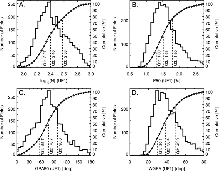
Figure 7. Histograms of the four key quantities measured for the UF1 stars in each of the GPIPS FOVs. Curves connecting diamonds are the cumulative probability distributions, with downward dashed lines locating the distribution quartile boundaries. (Top left, panel A): histogram of the base 10 logarithm of the number of UF1 stars in each GPIPS FOV. The median number of UF1 stars per Mimir FOV is 252. (Top right, panel B): distribution of median percentage polarizations (P50) for UF1 stars in each FOV. The median of this distribution is 1.53% at the H band. (Bottom left, panel C): distribution of median Galactic polarization position angle (GPA50) of the UF1 stars in each GPIPS FOV, where 90° represents a disk-parallel orientation. (Bottom right, panel D): distribution of interquartile ranges (WGPA) of the GPA distributions of the UF1 stars in each GPIPS FOV.
Download figure:
Standard image High-resolution imageTable 4. GPIPS FOV-based UF1 Polarization Distribution Properties
| Quantity | Quartile Boundary | ||
|---|---|---|---|
| First | Second | Third | |
| (1) | (2) | (3) | (4) |
| log10 N | 2.27 | 2.40 | 2.58 |
| P50 [%] | 1.30 | 1.53 | 1.80 |
| GPA50 [°] | 55.7 | 76.7 | 98.6 |
| WGPA [°] | 30.1 | 38.4 | 49.0 |
Download table as: ASCIITypeset image
The upper-left panel A in Figure 7 shows the distribution of numbers of UF1 stars in each FOV, binned by the base 10 logarithm of the number of star counts. The cumulative probability distribution is overplotted. As was done for the distributions in the GPIPS-1619 FOV, this cumulative distribution was analyzed to identify the quartile boundaries. The median number of UF1 stars in a GPIPS FOV is 252, while less than 25% of the FOVs have fewer than 188 stars and less than 25% have more than 378 stars.
The upper-right panel B of Figure 7 displays the histogram of the P50 (median debiased polarization percentage P') for UF1 stars in each of the GPIPS FOVs. The median of this distribution is 1.53%, with quartile boundaries at 1.30% and 1.80%. This median is only 1.06 times greater than the value found in an analysis of the first 18% of the GPIPS FOVs (DR1—Paper III). These polarization percentages are smaller than the optical wavelength values, which average closer to 5%–7% in the ISM (Hall 1949; Hiltner 1949a, 1949b). This difference is expected due to the wavelength dependence of starlight polarization (Serkowski 1973; Serkowski et al. 1975; Wilking et al. 1980).
The lower-left panel C of Figure 7 displays the distribution of median Galactic polarization position angles (GPA50) for the UF1 stars in each GPIPS FOV. As found in Paper III, the distribution is centrally peaked, though offset by 133 from the expected, disk-parallel value of GPA = 90° that characterizes most magnetic field models (e.g., Ferrière & Schmitt 2000). Over the region of the Galactic midplane surveyed by GPIPS in the first Galactic quadrant, the median magnetic field orientation is not purely parallel to the Galactic disk. It also exhibits broad orientation deviation wings that extend to both Galactic pole directions.
The lower-right panel D of Figure 7 shows the distribution of interquartile ranges (WGPA) of the UF1 GPAs of each individual GPIPS FOV. The distribution peaks near 30°–40°, with quartiles at 301, 384, and 490. These WGPA distributions in the GPIPS FOVs indicate that uniformly parallel magnetic fields are rare across 10' FOVs in the Galactic disk. This result has implications for assessments of the degree of magnetic or hydrodynamic turbulence and the ratios of energy density in the random and uniform magnetic field components (e.g., Jones 1989).
The offset of the median GPA from being purely disk parallel and the wide range of position angles present in each GPIPS FOV indicate that magnetic field models dominated by strongly uniform, disk-parallel behavior may not be adequate to describe these characterizations. In order to ascertain how these key properties vary with location in the Galactic disk, their one-dimensional (1D) and two-dimensional (2D) distributions were examined next.
4.3.2. Galactic Latitude and Longitude 1D Behavior of FOV-based Properties
The same four, FOV-based quantities for each GPIPS FOV, derived from the UF1 stars, are plotted versus Galactic latitude in Figure 8 and versus Galactic longitude in Figure 9. In both Figures, stacked plots are shown that display log N, P50, GPA50, and WGPA, respectively, from top to bottom. Black dots mark the values of each quantity measured for each of the GPIPS FOVs.
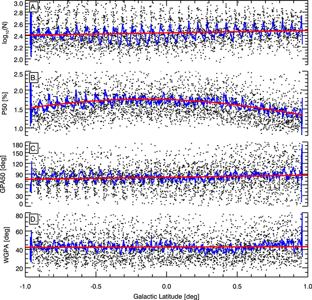
Figure 8. Galactic latitude variations of the four characterizing quantities measured for the UF1 stars in each of the GPIPS FOVs (black dots), running averages (10 point; blue lines), and best-fit lines or Gaussian (red lines—see the text). (Top, panel A) Base 10 log of the number of UF1 stars in each FOV. (Middle top, panel B) P50. (Middle bottom, panel C) GPA50. (Bottom, panel D) WGPA.
Download figure:
Standard image High-resolution image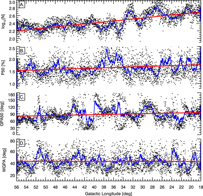
Figure 9. Galactic longitude variations of the four characterizing quantities measured in each GPIPS FOV (black dots), running averages (10 point; blue lines), and best-fit lines (red). (Top, panel A) Base 10 logarithm of the number of UF1 stars in each FOV—the Galactic bulge may contribute equal numbers of stars as does the Galactic disk from longitude 18° to about 34°, but there are strong variations on few-degree size scales. (Middle-top, panel B) P50. There are regions of coherent, high-percentage polarizations and a slow trend toward weaker percentage polarization as longitude increases (to the left). (Middle-bottom, panel C) GPA50. Regions of coherent, significant departures from the best-fit line, which itself swings from 95° to 80° for low to high longitudes, are present. (Bottom, panel D) WGPA shows no significant trend with longitude, though it has zonal departures.
Download figure:
Standard image High-resolution imageGalactic Latitude 1D Behaviors—In Figure 8, in addition to showing the black points for the FOV-based values, a 10 point running average is shown as the blue curve, a linear fit with latitude is shown in red for three of the four quantities, and a Gaussian fit with latitude is shown in red for the P50 plot. The top panel A shows that log N displays a strong, high-angular-frequency modulation (30 cycles over 2°) that is most easily seen in the blue running-average curve. This modulation is likely due to the slight variation of FOV Galactic longitude with latitude, related to the equatorial grid used to conduct the GPIPS observations (e.g., Figures 12–15, below). The modulation suggests that the log N dependence on longitude will be more pronounced than it is on latitude. Ignoring this modulation, the overall log N dependence on latitude appears to show a slight depression in star counts from about B = −06 to +01 (depicted by the blue, running-average means falling below the red linear fit), coupled with a weak rise in counts for positive latitude values (or a decrease in star counts for negative latitude values). The midplane decrease in counts is likely due to extinction by distant dust cloud complexes in the disk, which are expected to have small angular scale heights. The decrease in counts for negative latitude may be caused by extinction from more nearby clouds with larger angular offsets. The red line shows the linear fit, namely log10 N = (2.445 ± 0.004) + (0.041 ± 0.007) × GB, where GB represents Galactic latitude, in degrees.
The middle-top, panel B of Figure 8 that presents P50 also exhibits some of the same effects of the longitude beating. In addition, it also shows a weak rise in value, by about 0.2%–0.3%, centered near the midplane and falling toward the survey latitude limits. The data were fit with a Gaussian, returning an amplitude of 1.760% ± 0.011%, a Gaussian width of 153 ± 006, and center at GB = −0160 ± 0022. This polarization rise near the Galactic equator may be due to polarization contributed by more distant dust cloud complexes or ones with higher dust column densities.
The fitted Gaussian latitude width corresponds to a 36 FWHM, which, if associated with the 2.6 kpc median distance inferred for the UF1 stellar count density in the Figure 4 Gaia–GPIPS comparisons described earlier, implies an NIR polarization Galactic disk thickness FWHM of 160 pc, only ∼30% thicker than the 120 pc FWHM for the CO-traced gas layer (Clemens et al. 1988). A more realistic estimate might use half the distance to the UF1 star distribution as better representing the effective mean polarizing dust distance, resulting in an even thinner dust layer thickness and one in agreement with the CO layer thickness. Both estimates are thinner than the 400 ± 30 pc exponential scale height found for the Galactic magnetic field model developed by Jansson & Farrar (2012), based primarily on synchrotron RMs of extragalactic radio sources. For this GPIPS analysis, the apparently smaller NIR polarization scale height likely results from the combined effects of a larger magnetic field scale height and a smaller dust layer scale height.
The middle-bottom panel C of Figure 8, showing GPA50, also exhibits longitude beating, though with beat frequencies and amplitudes that change with latitude, suggesting complex longitude and latitude dependencies. The blue, running-average line segments and the red linear fit both exhibit means similar to the median in the histogram analysis described in Section 4.3.1. The linear fit gave a GPA50 value at GB = −1° of 754 ± 13, which rises to 867 ± 13 by GB = +1°. Hence, the median magnetic field orientation exhibits a weak mean dependence (5.7% ± 1.1% per deg) on latitude over the 2° sampled by GPIPS.
Finally, the bottom panel D of Figure 8 shows that WGPA exhibits weak longitude beating and almost no systematic variation with latitude. A linear fit returned a mean WPGA of 4263 ± 026 and a slope of 041 ± 047 of WGPA per degree of latitude. This result indicates that the significantly dispersed magnetic field orientation angles associated with WGPA values of 40° or more are common and do not disappear at any latitude within the GPIPS region. The black points at all latitudes do distribute along WGPA with the same pileup at low values and greater spread at high values characterizing the panel-D WGPA histogram of Figure 7. Thus, to first order, the relative incidences of coherent polarizations (low WGPA) and disordered polarizations are independent of Galactic latitude (but see Section 5.2.1, below).
Galactic Longitude 1D Behaviors—Figure 9 presents the same four FOV-based quantities versus Galactic longitude L, along with the same 10 point running averages as blue lines and linear fits as red lines. In all four of the panels in this figure, the quantities vary strongly and more coherently than they do with latitude GB (Figure 8).
The top panel A of log N in Figure 9 shows a rise in average numbers of UF1 stars per FOV toward lower Galactic longitudes, mostly for GL < 34°. This result was attributed in Paper III to the appearance of the Galactic bulge stars for these longitudes. Here, the ∼0.3 dex offset, between FOVs with GL > 34° and FOVs with GL < 34°, may indicate that the Galactic bulge contributes about the same number of stars to the GPIPS FOVs as are contributed by the Galactic disk, for FOVs with GL < 34°. The predominance of red giants in the bulge makes many of them detectable at the UF1 GPIPS sensitivity level, as predicted in Paper I and shown earlier in Section 4.1. This finding is another indication that UF1 stars probe to distances well into the bulge along these longitudes, likely in the 5–7 kpc range. In Figure 9(A), there are also some significant decreases in UF1 star counts, especially near longitudes 24°, 30°, 35°, 38°, and 51° and some apparent increases in star counts (e.g., near 21°, 27°, and 32°). The decreases span 05–2° of longitude and may be due to large complexes of dust (and gas) foreground to the bulk of the background stars seen in the neighboring fields. They could also represent interarm regions with fewer stars between richer spiral arms. A more detailed comparison of GPIPS star counts to star counts for Gaia and GLIMPSE as well as to 2MASS (H − K) colors is described in Section 4.3.3 below.
The middle-top panel B in Figure 9 shows a linear rise of P50 with decreasing longitude, though only by 0.24% ± 0.05% over the mean value of 1.53% ± 0.05%. Individual departures to higher and lower values far exceed this weak gradient. Some longitudes exhibit P50 decreases (e.g., 19°, 22°, 235, 27°, 33°, 405, 44°, 51°, and 55°) while others appear to have P50 increases (185, 205, 227, 25°, 35°, 38°, 48°, 53°). Whether P50 departures correlate with log N departures is examined in Section 4.4.1.
The middle-bottom panel C in Figure 9 shows that GPA50 exhibits the most dramatic variations with longitude. Defining any low-order polynomial trend was difficult. The red line, representing a linear fit, traces changes in the mean GPA50, from 951 ± 26 at longitude 18°, to 794 ± 41 at longitude 56°. However, the GPA50 values swing by 90° or more over longitude intervals as short as 2°–4°. The blue, 10 point moving averages also show that some GPA50 swings span nearly 180° over a few degrees of longitude, especially near longitudes 35°, 40°, and 52°. In contrast to the generally uniform behavior of GPA50 with Galactic latitude (Figure 8), the GPA50 longitude behavior is strongly nonuniform. Quantitatively, the 10 point moving averages deviate by more than 30° from disk-parallel orientations for over 30% of the longitude range surveyed (when averaged over latitude), compared to no such deviations for the latitude range survey (when averaged over all longitudes). Magnetic field orientation deviations in the disk midplane zone are mostly dominated by longitude effects and are nearly unaffected by purely latitude effects.
The bottom panel D in Figure 9 shows that WGPA exhibits the same lack of overall change with longitude that it exhibited with latitude in Figure 8(D). However, as for the previous three quantities, there are short intervals of longitude over which WGPA strongly deviates from the mean value, especially near longitudes 21°, 24°, 37°, 43°, and 52°. Two of these positive WGPA deviations, at 24° and 52°, correspond to longitude zones where large changes in GPA50 take place. Such rapid GPA changes could help drive WGPA to larger than average values. There also appear to be additional two- or three-way correlations, especially for longitude ranges 20°–21°, 36°–38°, 47°–49°, and 525–54°, where GPA50s are nearly disk parallel, P50 values are greater than average, and WGPA values are lower than average. These behaviors could be signaling the existence of regions of uniform, strong magnetic fields that are oriented parallel to the Galactic disk, an aspect explored further in Section 5.2.1.
These variations and correlations are intriguing and likely can help constrain models of the Galactic disk magnetic field. However, the lines of sight to individual GPIPS stars in each field can span quite different path lengths and encounter a variety of distinct dusty molecular clouds and/or spans of diffuse ISM. Interpretation of the variations must account for these line-of-sight differences.
4.3.3. Comparisons of Star Counts and Colors versus Longitude
Figure 10 shows the Galactic longitude behavior of the base 10 logarithm of the star counts in the Gaia g-band (top, panel A), Mimir POLCAT H band (middle top, panel B), and GLIMPSE 3.6 μm band ("L band"; middle bottom, panel C) as well as mean (H − K) colors from 2MASS (bottom, panel D) in 02 wide longitude bins. For the star count panels, stars were included if they appeared in the GPIPS FOVs and had photometric uncertainties under 0.33 mag. For the color panel, stars from 2MASS were included if their H and K magnitudes had uncertainties under 0.5 mag and the propagated (H − K) uncertainty was under 0.33 mag. The colors of the 2MASS stars meeting these criteria in each longitude bin were averaged without weighting to produce mean color values. The green dashed line in each panel indicates an unweighted fit to the values. The resulting slopes suggest e-folding (decrements by 0.43 dex) longitude spans of 84° for the g band and 36° for the H and L bands. These imply that Gaia star counts do not include many stars that are as distant as the Galactic bulge, while the GLIMPSE L-band counts do. The Mimir H-band POLCAT star counts exhibit the same slope as does the GLIMPSE L band, indicating that POLCATs include bulge stars.
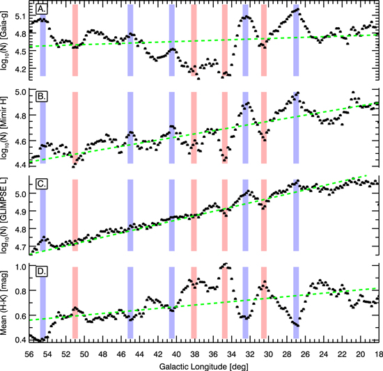
Figure 10. Comparison of star counts and colors for Gaia, Mimir, GLIMPSE, and 2MASS. In all panels, binned data points are shown as black symbols, unweighted fits with longitude are shown as dashed green lines, and local regions with changes in properties are identified by vertical light-red or light-blue rectangles. The top, panel A, presents the base 10 logarithm of the numbers of Gaia stars found in the GPIPS FOVs and having g-band magnitude uncertainties under 0.33 mag. The middle top, panel B, presents similar star counts for Mimir H-band DR4 POLCAT stars. The middle bottom, panel C, shows the star counts for GLIMPSE 3.6 μm ("L"-band) stars. The bottom, panel D, shows the run of unweighted mean (H − K) stellar colors, from 2MASS. The photometric tracers show decreases in star counts with increasing longitude, while the colors become less reddened with increasing longitude. The light-red vertical rectangles show the correlation of localized redder star colors with star count decrements. The light-blue rectangles show where less-reddened stellar colors correspond to local increases in star counts.
Download figure:
Standard image High-resolution imageVertical light-red and light-blue rectangles identify longitudes where color and star count changes are correlated. Light-red rectangles at longitudes 305, 3475, 38°, and 51° are where the (H − K) colors become redder and the star counts in the photometric bands strongly decrease. Light-blue rectangles at longitudes 27°, 325, 405, 47°, and 545 show where the (H − K) colors become less red and the star counts correspondingly increase. Strong color changes due to changes in spatially distributed stellar populations (e.g., disk versus bulge stars) are not expected. Instead, where the colors become redder, more dust extinction must be present along the line of sight to the stars, likely associated with molecular cloud complexes and/or Galactic spiral arms. Interestingly, where the colors are less red, there must be a corresponding relative deficit of extinction along these sight lines, resulting in more stars being revealed and perhaps seen to greater distances. These modulations are strongest for longitudes between 25° and 40° and beyond 54°, with all tracers participating. Outside of these regions, the GLIMPSE L-band star counts, in particular, show only smooth bin-to-bin behavior.
4.4. Correlated Behaviors of FOV-based Properties
To explore the nature of possible correlations among the four key characterizing quantities, a corner-plot representation was developed, using the median-value characterizations for each of the GPIPS FOVs, and is shown in Figure 11. For each of the six panels in the figure, their 2D spans were gridded uniformly into 31 × 31 bins and the number density of GPIPS FOV values in each bin was found. Where the FOV counts in bins were high, open and filled contours were added to convey isodensity locations and changes.
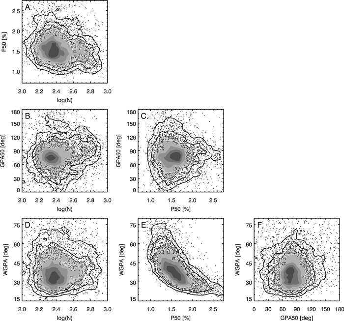
Figure 11. Corner-plot comparisons of key polarization properties for the FOV-based, median-value quantities in the GPIPS FOVs. In each panel, individual FOV values are shown as black dots until the density of dots becomes high. Thereafter, open and filled contours continue the density representation, stepped linearly with point density by 12.5% of the peak value, starting at that 12.5% value. (Upper left, panel A): P50 vs. log N. (Middle left, panel B): GPA50 vs. log N. (Middle center, panel C): GPA50 vs. P50. (Lower left, panel D): WGPA vs. log N. (Lower center, panel E): WGPA vs. P50. (Lower right, panel F): WGPA vs. GPA50.
Download figure:
Standard image High-resolution imageThe upper-left panel A in Figure 11 shows how P50 and the log of the number of UF1 stars in each field are related. There is a peak likelihood at about 1.5% for P50 and 240 stars per field (log N ∼ 2.37) with Gaussian-like decays away from the peak. There is a weaker, secondary peak at 1.5% in P50 and log N ∼ 2.7, which comes from the longitude range less than 34°, as it is only in that range that such high UF1 star counts are seen in Figure 9. This local increase could be due to distant bulge stars. There is also a minor tertiary peak at 1.25% for P50 and 2.8 for log N, which corresponds to the L = 27° count increase and polarization dip seen in Figure 9.
The middle-left panel B in Figure 11 compares GPA50 with log N, revealing the likelihood peak at 75° of GPA50 and 210 stars per field. The secondary and tertiary peaks noted appear to blend into one weaker peak near GPA50 = 90° and log N = 2.7.
The middle-right panel C in Figure 11 compares GPA50 with P50, showing a likelihood peak at about 1.7% and 77°, respectively. Near 1.4% of P50, the GPA50 values extend from 0° to 180°, suggesting that angle aliasing may be present. As the P50 values increase beyond 1.5%, the GPA50 range decreases and GPA50 values appear to move closer to a disk-parallel (GPA = 90°) orientation. There are few fields with P50 values below 1%, as was already shown in Figure 7(B), and this could be a consequence of the UF1 selection criteria.
The lower-left panel D in Figure 11 examines how the widths of the GPA histograms in each FOV, WGPA, depend on the numbers of UF1 stars in those FOVs. The likelihood maximum is at about 240 stars per FOV and 33° of WGPA. The number of UF1 stars in an FOV does not appear to constrain WGPA, as the latter shows values extending to 75° or beyond for log N values similar to those at the peak. The weak secondary and tertiary log N peaks from panel A appear here with slightly higher WGPA values than for the main peak, perhaps as high as 40°–45°.
The lower-center panel E in Figure 11 shows a strong anticorrelation of WGPA and P50, which was suggested in the discussion of the previous section. While there does appear to be a likelihood peak near 1.7% and 35°, the overall curved shape of the contours indicate some degree of correlation. For GPIPS FOVs exhibiting high median polarization fractions, the widths of their polarization position angle distributions are narrow, as small as 15°–20°. On the other hand, the fields showing the widest GPA distributions exhibit the weakest P50 values, as small as 1%–1.25%. Such anticorrelations of polarization with dispersion in position angle have been seen elsewhere (Planck Collaboration et al. 2015, 2018) and are examined in more detail in Section 5.2.
The lower-right panel F in Figure 11 compares WGPA to GPA50. The likelihood maximum has a center near 76° of GPA50 and 36° of WGPA. The contours appear mostly symmetric across GPA50 and not symmetric along WGPA. The lack of correlation between WGPA and GPA50 here and the lack of correlation between GPA50 and P50 (panel C) indicate that the anticorrelation of WGPA and P50 (panel E ) is the fundamental dependence. The mean orientation of the magnetic field in the plane of the sky has no bearing on the anticorrelation of polarization percentage with the width of the GPA distribution (or, equivalently, dispersion of PAs).
4.4.1. Latitude and Longitude 2D Behavior of FOV-based Properties
This section presents the 2D distributions of the FOV-based polarization properties of log N, P50, GPA50, and WGPA for the GPIPS UF1 stars. Due to the large aspect ratio of longitude coverage to latitude coverage of GPIPS, the 2D representations are shown as stacked longitude slices with aspect ratios chosen to retain sky-true shapes and orientations. In all cases, color look-up rectangles are shown, labeled with limiting values, and have gray bars indicating the corresponding values of the contours that are overlaid on the images. Each of the GPIPS FOVs is shown as a rotated square to emphasize the equatorial orientation of the Mimir instrument. Each is placed at the equatorial grid center used for the GPIPS observations. Appendix D presents alternative representations of the same figures, using color look-up tables better suited to individuals with color vision deficiency (CVD).
Log N versus Galactic longitude and latitude—Figure 12 presents a false-color representation of the log N counts of UF1 stars in each GPIPS FOV as functions of Galactic latitude and longitude, for four stacked longitude slices. Each longitude slice spans 10°, starting with the lowest longitude surveyed (18°) at the rightmost limit of the lowest slice in Figure 12, and proceeding from right to left and then up to the next slice until the final survey longitude of 56° is reached. Each longitude slice presents the full 2° latitude extent of the survey. The color-table look-up rectangle in the uppermost slice indicates that the least populous FOVs, shown in the darkest blue colors, contain about 80 UF1 stars on average (log N = 1.9). The most populous FOVs, shown in red colors, contain 1000 or more UF1 stars. The general increase in the number of UF1 stars for GL < 34° is likely due to the contribution of bulge red giant stars in addition to the disk stars sampled at all longitudes, as noted earlier.
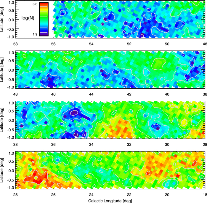
Figure 12. False-color representation of the base 10 log of the number of UF1 stars in each of the GPIPS FOVs, vs. Galactic longitude and latitude, as four longitude slices. Color look-up rectangle, with six nearly equally spaced gray contours, corresponding to 100, 150, 225, 340, 500, and 750 UF1 stars per FOV, is shown in the top slice. The smallest number of UF1 stars in any FOV is 64, the largest is 1112. Note that extinction and the Galactic bulge both likely play roles in the variations in the numbers of detected stars with direction. (Also shown as Figure D1 for CVD individuals.)
Download figure:
Standard image High-resolution imageIn Figure 12, three extended zones of enhanced numbers of UF1 stars in the FOVs are apparent. These span Galactic longitudes 18°–215 for positive latitudes down to midplane ones, longitudes 24°–29° for mostly negative latitudes (though with a small secondary peak to positive latitudes at longitude 275), and from longitudes 319–332 for only negative latitudes. These three zones appear to account for the three peaks in the run of log N versus longitude in the lowest panel of Figure 9 and in the photometric panels (A, B, C) of Figure 10. Similarly, reductions in the numbers of stars per FOV for large, resolved regions near longitudes 305, 35°, 375–39°, 42°–44°, 46°, and 51° correspond to specific dips in the log N versus longitude curve in Figures 9 and 10. The patterns of high and low numbers of UF1 stars seen in the different GPIPS FOVs are likely due to the extinction effects described earlier regarding Figure 10, but here they are resolved in longitude and latitude.
P50 versus Galactic longitude and latitude—The Galactic longitude and latitude distribution of UF1 median percentage polarization P50 is shown for the GPIPS FOVs in Figure 13. The false-color mapping scheme spans from about 0.8% to 3.0%, though the maximum value across the map is closer to 5% and the average is about 1.5% (Figure 7(B)). Regions of polarization percentage greater than that average (light-blue to green colors) tend to be found closer to the midplane. Comparing Figures 12 and 13, the zones of higher star counts in Figure 12 are seen in Figure 13 to exhibit lower median polarization percentages (e.g., longitudes 32°–33°, latitudes ≤0°). The reverse is also true—lower star count regions tend to exhibit higher polarization percentages (e.g., longitude 306, latitude −04), likely the signature of dust along those latter sight lines both extincting and polarizing the background starlight. This trend is more pronounced in Figure 13 than in Figure 11(A), so seeing the trend in Figure 13 helps reveal the weak anticorrelation of log N with P50 that is present in Figure 11(A).
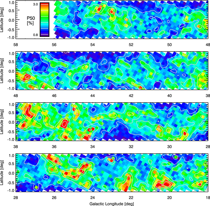
Figure 13. Galactic longitude and latitude distribution of the median percentage polarization P50 in each GPIPS FOV. Polarization medians range from around 0.8% to over 3% in the H band, with a weak tendency to be higher along the disk midplane. Six gray contour levels corresponding to P50 values of 0.9%, 1.3%, 1.7%, 2.1%, 2.5%, and 2.9% are drawn over the false-color panels and inside the color look-up rectangle in the top panel. (Also shown as Figure D2 for CVD individuals.)
Download figure:
Standard image High-resolution imageThe roughly 25–30 regions showing the greatest polarization percentages (red colors) in Figure 13 have small angular extents. They also tend to be surrounded by regions of higher than average polarization (green colors), which are themselves more extended. The natures of these high-P50 regions are explored further in Section 5.2.
GPA50 versus Galactic longitude and latitude—The Galactic midplane distribution of GPA50 values at 10' resolution is shown as Figure 14. There, the color look-up conversion has been modified so that GPA50 values of 0° and 180° are represented by the same false color in order to reduce display confusion caused by angle aliasing. The colors representing Galactic disk-parallel magnetic field orientations are close to the green-blue false-color boundary. A red contour, which corresponds to GPA 90°, is shown. Some large regions of the stack of longitude slices do appear dominated by colors that are mostly green to blue and so have GPA50 values similar to being disk parallel.
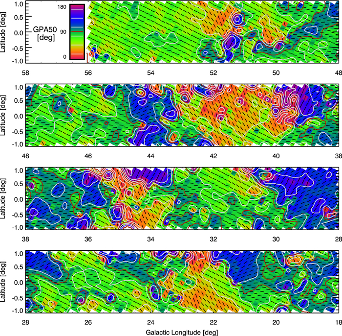
Figure 14. Galactic longitude and latitude distribution of GPA50 in each GPIPS FOV in the same four-slice presentation as in the previous figures. Note that the look-up table colors wrap around 0° and 180° to reduce the appearance of aliasing. Black lines within each FOV box indicate the GPA orientation. Six gray contour levels, corresponding to GPA50 values of 15°, 45°, 75°, 105°, 135°, and 165°, and one red contour, corresponding to the disk-parallel GPA50 value of 90°, are drawn over the false-color panels and inside the color look-up rectangle in the top panel. (Also shown as Figure D3 for CVD individuals.)
Download figure:
Standard image High-resolution imageHowever, there are also several regions that exhibit GPA50 values that are far from being disk parallel. The larger regions span longitudes of 21°–23°, 335–36°, 39°–43°, and 50°–525. The first two of these regions correspond to the two dips in GPA50 seen in Figure 9. The region near longitude 22° appears to be a fairly uniform zone showing GPA50 values of 40°–45° and could be due to the magnetic field characterizing a single molecular cloud or complex. The feature near longitude 34° is more complex, seemingly consisting of extended zones above and below the Galactic equator. The negative latitude zone is similar in characteristics to the longitude 22° zone, but the positive latitude zone is different in that it shows strong GPA50 variations across a ridge of nearly constant R.A.
WGPA versus Galactic longitude and latitude—Figure 15 presents the Galactic midplane distribution of the final key quantity, WGPA, the interquartile ranges of the UF1 star GPA distributions in each GPIPS FOV. In this figure, the color table is reversed to associate lesser WGPA values (those exhibiting greater GPA coherence) with red colors and greater WGPA values with darker, bluer colors. The Davis–Chandrasekhar–Fermi (DCF: Davis 1951; Chandrasekhar & Fermi 1953) method for estimating magnetic field strengths from linear polarization data has an inverse dependence on polarization position angle dispersion, a direct linear dependence on gas velocity dispersion, and a square root dependence on gas density. Assuming the latter two quantities exhibit roughly constant mean values across all FOVs (a weak, but useful first step), the red highlighted zones in Figure 15 could represent regions of locally stronger magnetic field strength. In Figure 15, the overall impression is one of a relatively uniform background of WGPA values near 31° (green colors; ΔGPA ∼ 13°), with many small regions and 9–10 larger regions of low-WGPA values, seen as red-colored zones. High-WGPA values are present in many small zones and a few larger zones, but in fewer numbers of regions, both small and large, than for the low-WGPA zones. Low-WGPA FOVs correlate with high-P50 FOVs, as already noted in the discussion related to Figure 11(E) and as examined in Section 5.2
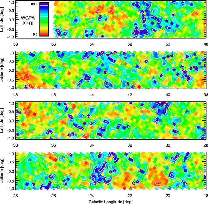
Figure 15. Galactic longitude and latitude distribution of WGPA, the interquartile ranges of the GPA distributions in each of the GPIPS FOVs. The color look-up rectangle in the uppermost panel indicates that WGPA values range from a low of about 15° (red colors) to a high of about 80° (dark blue colors). Six gray contour levels corresponding to WGPA values of 20°, 31°, 42°, 54°, 64°, and 75° are drawn over the false-color panels and inside the color look-up rectangle in the top panel. Note that the value to color mapping in this figure is inverted from previous figures to highlight the low-WGPA regions in red. (Also shown as Figure D4 for CVD individuals.)
Download figure:
Standard image High-resolution image5. Discussion and Applications
The types of studies made possible by GPIPS data will be different in nature and scope than those performed using other existing magnetic field probes. The data contained in GPIPS DR4 include more than 1 million measured stellar polarizations of high quality that have the potential for being used individually (UF1 type; Paper III). The UF2 and UF3 stars account for another nearly 9 million stars, but need careful distance selection and averaging to return magnetic field information. Planck polarization at 353 GHz, with its 5' resolution, yields about 6 million independent samples across the entire sky, but only 11 thousand across the GPIPS zone. The pulsar and extragalactic radio source list used by Han et al. (2018) for characterizing the magnetic field of the Galactic disk via RMs includes 4700 sources, but spans eight times the latitude range and 9.5 times the longitude range of GPIPS. If those sources were uniformly distributed in latitude and longitude (a poor, but serviceable assumption—see Han et al. 2018), then only about 60 of these sources probe lines of sight through the GPIPS region. Hence, whether compared to the sampling density of the radio continuum magnetic field RM studies (0.8 samples deg−2) or to Planck thermal dust emission from the Galactic plane (183 beams deg−2), GPIPS data achieve much finer angular sampling (14,400 UF1 stars deg−2) than any other technique.
The science applications of the GPIPS data will likely be many and are well beyond the scope of this introductory presentation. GPIPS data from earlier data releases have been used to create the first resolved map of the plane-of-sky magnetic field strength for a molecular cloud (Marchwinski et al. 2012) and used with deeper K-band (2.2 μm) Mimir polarimetry to map the magnetic field strength across an infrared dark cloud (Hoq et al. 2017).
In the following, example studies based on comparisons of GPIPS to Planck yielded some new findings and insights. The first comparison involved the plane-of-sky polarization position angle orientation distributions of Planck and GPIPS. The second was a deeper look at the anticorrelation of WGPA and P50.
5.1. Plane-of-sky Polarization Orientation Distributions Comparison
The histograms of the Galactic polarization position angle using GPIPS NIR background starlight polarimetry were shown in Figure 24 of Paper III and here in Figure 7(C). The first was constructed from values measured in the DR1 GPIPS release of 50,000 stars of UF1 type with the additional criterion of requiring P'/σP ≥ 2.5 to select higher-quality measurements. The resulting histogram of the numbers of such stars versus GPA revealed a single peak at about GPA = 75° with an FWHM width of about 50°.
Here, using GPIPS DR4, the distribution of the FOV-based median values derived from the GPA distributions for the UF1 stars in each of the GPIPS FOVs was presented in Figure 7(C). There, the median of the GPA50 distribution is 767, with an interquartile range of about 43°. So, while the distribution of GPA50 values appears to be somewhat narrower than the corresponding distribution of high-quality DR1 GPIPS star GPA values, the distribution centers are similar.
For Planck 353 GHz polarization, Planck Collaboration et al. (2015) showed, in their Figure 3, the distribution of GPAs with, and without, bandpass correction terms. When corrected using their favored approach, the GPA distribution for the first Galactic quadrant (longitudes 0°–90°, encompassing the GPIPS region) shows a peak at a GPA equivalent8 of about 95° and an FWHM of about 40°. Their PA distribution shows the same asymmetry of lower likelihoods for GPAs greater than 90° and higher likelihoods for GPAs less than 90°, as seen in the GPIPS distributions. Thus, the Planck results disagree in mean or median GPA values with respect to GPIPS by about one-half of the distribution widths, although the distribution shapes appear to be similar.
More recently, Planck Collaboration et al. (2018), in their Figure 6, reported a 353 GHz GPA histogram for the entire sky, computed for 80' resolution, that peaks at about 86° and has an FWHM of about 40°. This is closer to the ∼77° value found in GPIPS data, but still differs by 9°.
The exact reason for the difference in GPA distributions between GPIPS and Planck remains unknown. It could arise from differences in the effects of angular resolution and/or the line-of-sight distances probed. The GPIPS angular sampling is orders of magnitude finer than Planck achieves, so GPIPS could be resolving structures that are too small to be resolved by Planck. However, many of the features found here in the GPIPS 2D (e.g., Figure 14) and 1D (e.g., Figure 9) plots span angular sizes that are much larger than the Planck polarization resolution. Line-of-sight effects could be causing Planck beams to integrate dust emission over much longer distances than are probed using GPIPS, again leading to smoothing of GPIPS-resolved changes by the Planck observations and analyses. GPIPS findings, derived from polarizations of background stars, will necessarily be limited in the line-of-sight distances that can be probed, as stellar faintness and extinction both contribute to detection limitations (Paper I, and Section 4.1, above). However, the presence of the Galactic bulge in the GPIPS stellar distributions (Figures 9 and 12) shows that the GPIPS far horizon must extend to at least 5–7 kpc from the Sun.
The question of exactly why GPIPS and Planck differ in their inferred GPA distributions remains unanswered and may have to wait until robust models of the Galactic magnetic field, at spatial and angular resolutions finer than currently exist, become available for testing.
5.2. The Anticorrelation of WGPA and P50
The anticorrelation of WGPA and P50 seen in Figure 11(E) has been seen previously in Planck polarization data (e.g., Figure 23 of Planck Collaboration et al. 2015) and perhaps in SCUBA submillimeter polarization data even earlier (Poidevin et al. 2010). More recent Planck analysis (Planck Collaboration et al. 2018) used a larger region of the sky over which to find a width–polarization relation they argued was of the form S × P = constant, where S is a measure of the polarization position angle dispersion and P is the fractional polarization measured at 353 GHz.
In Planck Collaboration et al. (2018), an analytic model was constructed using Gaussian fluctuations containing combinations of uniform and random (turbulent) magnetic fields for multiple zones along the line of sight to test the observed S × P relation, and a strong anticorrelation was found between S and P. They argue that this anticorrelation is a direct result of magnetic field topology and should be a general property of the Galactic magnetic field.
To examine whether GPIPS was also returning similar results, the plot of WGPA versus P50, which should be closely equivalent to the S versus P plots in the Planck papers, was recast in the log–log form used in the Planck papers and is presented as panel A of Figure 16. There, each black dot is plotted at the log-based location corresponding to the median UF1 polarization (P50) and the interquartile range (WGPA) for one GPIPS FOV. The red line represents the best-fit robust linear regression, resulting in a slope of −1.266 ± 0.014. This power-law index is similar to the −1 value dictated by the S × P relation. But, the measured index misses negative unity by almost 20 times its uncertainty. While the GPIPS data appear to be generally consistent with the Planck findings, there are key differences.
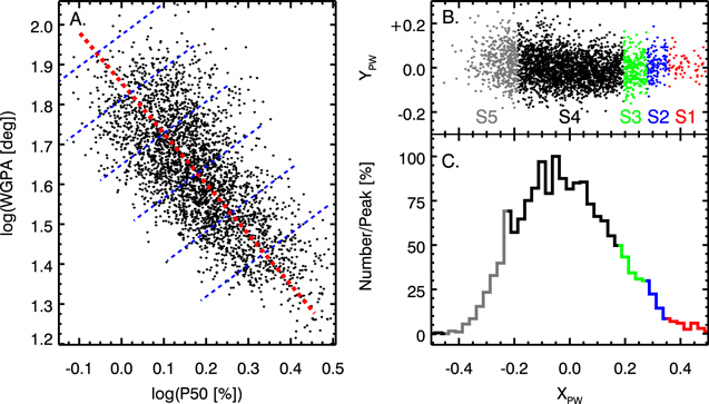
Figure 16. The WGPA-P50 anticorrelation and the five selected subsamples of GPIPS FOVs. (Left, panel A): distribution of GPIPS WGPA and P50 FOV-based data values, plotted in base 10 log–log format. Black dots correspond to the WGPA and P50 values of the individual GPIPS FOVs. The red dashed line represents the robust linear regressed line. Dashed blue lines oriented perpendicular to the red line indicate notional binning of data into bins spaced along the red line. (Right upper, panel B): same distribution of WGPA and P50 data points as for panel A, after rotating and shifting to make the regressed linear-fit line centered and horizontal (see text). Data points are colored red, blue, green, black, and gray to indicate the data subsample to which they were assigned—red for the S1 highest-P50/lowest-WGPA FOVs subset through the other colors to gray for S5, representing the lowest-P50/highest-WGPA FOVs subset. (Right lower, panel C): histogram of the numbers of GPIPS FOVs falling into 41 bins along the XPW-axis. Histogram colors are the same as for the data points in panel B.
Download figure:
Standard image High-resolution image5.2.1. Locating Strong and Weak Magnetic Field Regions
In Planck Collaboration et al. (2015), the highest PA-dispersed regions were argued to form boundaries between isolated segments characterized by high-P values and low-PA dispersions (their Figure 22(top)). These isolated segments could represent regions of greater magnetic field strength, or at least greater magnetic field orientation coherence. The sizes of the isolated Planck segments appear to be a few degrees. Because GPIPS data exhibit a similar anticorrelation of S and P, the question of whether similar isolated segments of low PA dispersion are surrounded by high PA-dispersion regions in GPIPS was examined to try to learn about these potentially magnetic-dominated zones.
The panel-A distribution in Figure 16 was divided into five subsamples of GPIPS FOVs that spanned low- to high-P50 values. This division was performed in a way that was equivalent to collecting the panel-A distribution into bins oriented perpendicular to the red line, as suggested by the dashed blue lines in that panel. Such binning respects the S × P anticorrelation while retaining sensitivity to differences in the magnetic field properties of the GPIPS FOVs along the correlation direction. The method involved rotating the distribution of panel A points to cause the red line of the correlation to become horizontal, resulting in the FOV distribution shown in panel B of Figure 16. Through this rotation, the new axes (XPW and YPW) became linear combinations of P50 and WGPA and thereby carried mixed units. In panel B, the GPIPS fields are mostly distributed horizontally without much coherent curvature of YPW on XPW. As a result, the GPIPS FOVs became primarily distributed along the new x-axis, which maximally separated FOVs with high-P/low-WGPA from FOVs with the opposite behavior. Figure 16 panel C shows a normalized histogram, after marginalizing over YPW, with the rotated axis XPW as the new indicator of likely magnetic field strength or coherence.
Five subsamples of the rotated GPIPS FOV values were selected. These probed the magnetic nature of the high-P50/low-WGPA FOVs using three of the subsamples, the low-P50/high-WGPA FOVs with one subsample, and collected the remaining (moderate-P50/moderate-WGPA) FOVs into one reference subsample. The most highly polarized, and least PA-dispersed, subsample of GPIPS FOVs was chosen to be the 64 FOVs (∼2% of the total in the full distribution) with the most positive XPW values in Figure 16(C). This subsample was designated S1 and those FOVs are colored red in panels B and C. The 129 next-most highly polarized GPIPS FOVs (∼4%) comprised the S2 subsample and are colored blue. The 258 GPIPS FOVs (∼8%) beyond S2 became the S3 subsample and are colored green. At the other end of the histogram, a subsample of 452 GPIPS FOVs (∼14%—equal in size to the the total of the S1, S2, and S3 subsamples) containing the least polarized and most PA-dispersed FOVs was designated S5 and its FOVs are indicated in gray. The remaining 2334 GPIPS FOVs (∼72%) in the middle of the distribution were designated S4 and are colored black to identify the non-extreme, more average behaviors of their FOVs.
Multidimensional Analysis of Coherent High-P/Low-WGPA Structures—Figure 17 offers a two-fold comparison of the relative locations of the S1, S2, and S3 high-P50/low-WGPA selected FOVs (red, green, and blue points, respectively) and the S5 low-P50/high-WGPA selected FOVs (gray points). The top, panel A, of Figure 17 presents the Galactic longitude and latitude distributions of those FOVs. There appear to be many distinct clumps of multiple GPIPS FOVs exhibiting high-P50/low-WGPA values. The largest of these clumps show central cores comprised of S1 (red) points surrounded, or bordered, by S2 (blue) and S3 (green) FOV points. Under the assumption of rough uniformity of gas velocity dispersion and density over FOV sizes, these could signify zones of high magnetic field strength being embedded in somewhat weaker field regions. Alternatively, they could signify zones where the magnetic field is purely in the plane of the sky and so maximizes P50 values and minimizes WGPA ones, while being surrounded by regions of more mixed, less uniform, magnetic field inclination angles.
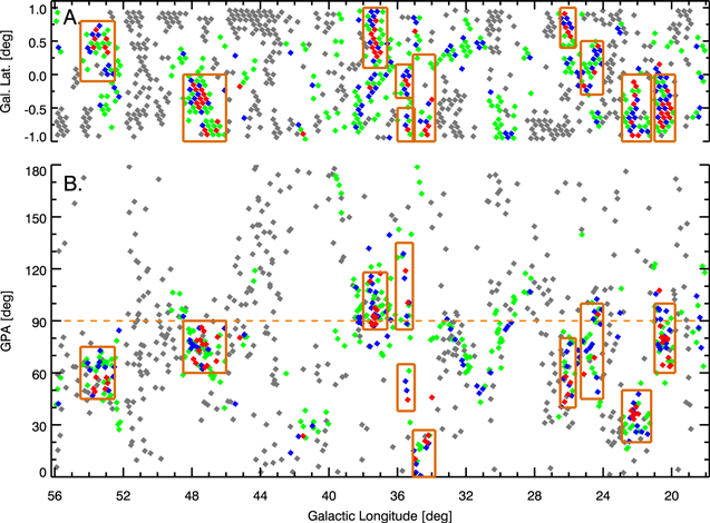
Figure 17. Multidimensional distributions of the (strong field) S1, S2, S3, and (weak field) S5 subsamples of GPIPS FOVs. (Top, panel A): Galactic longitude and latitude locations of the subsample FOVs. The S1, S2, and S3 (red, blue, and green) FOVs appear to group into distinct structures while the S5 (gray) FOVs mostly form structures at the latitude limits of GPIPS. (Middle, panel B): median GPA vs. Galactic longitude for the subsample FOVs. The spatial coherence seen for the S1, S2, and S3 FOVs in the top panel is also present as coherent GPA values for each distinct structure in the lower panel. This is not the case for the S5 (gray) FOVs, which show much less GPA clustering. Light-brown rectangles indicate the extents of the 10 groups described in the text and listed in Table 5.
Download figure:
Standard image High-resolution imageThe S5 (gray) FOV points also show multiple resolved regions, but these tend to be located mostly at the Galactic latitude limits of the survey region. As these zones contain somewhat fewer UF1 stars and lower P50 values, the S5 regions could represent either lower extinction zones, weaker magnetic field zones, or zones with more random magnetic field orientations and/or inclinations.
There does appear to be a rough anticorrelation of S5 fields with the S1, S2, and S3 fields in longitude and latitude space, but concluding that the high-WGPA S5 fields are defining boundaries around, or between, low-WGPA S1, S2, and S3 fields seems unsupported in these GPIPS data. Instead, the high-P zones appear to be surrounded by more average (e.g., S4—not shown in these plots for clarity) magnetic field strength (or orientation coherence) regions.
The bottom, Figure 17, panel B, shows GPA values versus Galactic longitude locations of the FOVs. Many of the same groupings of colors remain coherently located in this plot. Thus, these regions of higher-P50/lower-WGPA appear to be associated with resolved, coherent magnetic fields, at least locally, that have nearly constant plane of sky orientations (GPAs).
Resolved Strong-field Regions—In order to obtain some quantitative evaluation of this clustering behavior and to locate these potentially strong magnetic field regions, coherent groupings of points were identified visually in Figure 17. Groups needed to exhibit agreement in subsample designation (S number or plotted color), Galactic longitude and latitude, and GPA so as to remain identifiable as distinct clumps. Subjectively, there appear to be about 10 such large groups, each of which has multiple high-P50/low-WGPA (strong B-field) S1 (red) FOVs, many S2 (blue) FOVs, and many S3 (green) FOVs. There are also some lesser groups that have one or no S1 FOVs. The longitude and latitude center locations as well as angular and GPA spans for the 10 major groups are summarized in Table 5 and are shown as light-brown rectangles in Figure 17.
Table 5. High-P/Low-WGPA Groups of Potentially Strong Magnetic Fields
| Number | Designation | Galactic Ranges of | GPA Range | N(FOVs) | |
|---|---|---|---|---|---|
| Longitude | Latitude | (S1+S2) | |||
| (°) | (°) | (°) | |||
| (1) | (2) | (3) | (4) | (5) | (6) |
| 1 | L20.5 | [19.8, 21.0] | [−1.0, 0.0] | [60, 100] | 22 |
| 2 | L22.0 | [21.2, 22.9] | [−1.0, 0.0] | [20, 50] | 16 |
| 3 | L24.5 | [24.0, 25.3] | [−0.3, +0.5] | [45, 100] | 13 |
| 4 | L26.0 | [25.6, 26.5] | [+0.4, +1.0] | [40, 80] | 9 |
| 5 | L34.3 | [33.8, 35.1] | [−1.0, +0.3] | [0, 27] | 7 |
| 6 | L35.3A | [35.0, 36.0] | [−1.0, −0.5] | [38, 65] | 3 |
| 7 | L35.3B | [35.1, 36.1] | [−0.35, +0.15] | [85, 135] | 7 |
| 8 | L37.5 | [36.6, 38.0] | [+0.1, +1.0] | [85, 118] | 17 |
| 9 | L47.5 | [46.0, 48.5] | [−1.0, 0.0] | [60, 90] | 23 |
| 10 | L53.5 | [52.5, 54.5] | [−0.1, +0.8] | [45, 75] | 15 |
Download table as: ASCIITypeset image
In Table 5, the first column is a group sequence number, ordered by increasing Galactic longitude. The second column offers designations, based on the mean Galactic longitude of the group. The next column lists the longitude range spanned by each group, followed by the latitude range spanned. The fifth column lists the GPA range spanned. The sixth column lists the total number of the highest-P S1 (red) and S2 (blue) GPIPS FOVs contained within each group. These two extreme FOV types appear to be more clustered in panels A and B of Figure 17 than do the S3 (green) FOVs and so were chosen to define the group extents and contents.
The total number of S1 and S2 GPIPS FOVs contained within the 10 groups is 132. This is about 68% of the total number of S1+S2 FOVs. That is, the highest-P50/lowest-WGPA FOVs appear to be the most clustered class of FOVs. This would seem to argue that resolved regions with strong magnetic fields are not uniformly distributed but instead are localized to perhaps 10–12 major structures. The average S1+S2 FOV count per group is about 13. For circular groups, this is equivalent to a diameter projection spanning about 04, or 18 pc for an average assumed distance of 2.6 kpc (see Section 4.1). While it is possible that these groups represent just the highest-P50 centers of larger coherent structures, it is difficult to imagine that the groups found here also happen to be located within structures having sizes of several degrees, as the Planck analyses (Planck Collaboration et al. 2015) would suggest.
The remaining 2334 S4 GPIPS FOVs (72%), colored black in the right panel of Figure 16, were also plotted in the same form as for the high- and low-P50 fields shown in Figure 17. Those S4 fields, exhibiting more typical values of P50 and WGPA, were found to be mostly uniformly distributed in Galactic longitude and latitude, absent the regions already selected by the high- and low-P50 fields. The average fields were also distributed somewhat uniformly along the GPA plot, though following the trends seen in Figure 9(C), with no groupings as obvious as those listed in Table 5.
Thus, the S5 (gray; low P50) fields seem to mostly occupy the survey latitude boundaries, the S1, S2, and S3 high-P50 fields (red, blue, green) are mostly found in about 10 resolved groupings, and the more moderate-P50/WGPA FOVs are fairly uniformly distributed.
The positions and extents of the 10 high-P50 groups listed in Table 5 were compared to the positions and extents of previously cataloged star formation regions in the GPIPS zone to ascertain whether star formation correlates with high-P50/low-WGPA (strong magnetic field) conditions. The regions tabulated by Murray & Rahman (2010) that showed strong thermal free–free emission, as detected by WMAP and correlated with GLIMPSE and Midcourse Space Experiment MSX (Price et al. 2001) images, include 11 within the GPIPS zone. Similarly, the catalog of Red MSX Sources (RMS: Urquhart et al. 2014) lists 15 luminous, and presumably massive, young stars in the GPIPS region. The agreement with the GPIPS group list of Table 5 was weak—4 of 11 for the WMAP regions and only 2 of 15 for the RMS objects. Some of these massive star-forming regions are also likely at distances too great for GPIPS to have been able to probe. The generally poor matching of high-P/low-WGPA regions with zones of massive star formation may indicate that strong and/or uniform magnetic field conditions are not prevalent in such settings.
Are these high-P50/low-WGPA groups physical objects with strong magnetic field strengths, or are they regions where the magnetic field just happens to be well aligned and mostly in the plane of the sky? Establishing magnetic field strengths for the regions rests on application of the DCF method and thereby requires high-quality information for gas velocity dispersions and gas volume densities across the regions, or Zeeman effect high-resolution and high-sensitivity molecular line spectroscopy. These are beyond the scope of this paper, but should be pursued.
5.2.2. GPA Distribution Comparison
Do regions of strong (or uniform) magnetic fields, as delineated by the high-P50/low-WGPA FOVs in GPIPS, show mean Galactic polarization position angles that are distinct from the other, more typical, GPIPS FOVs? To try to answer this question, Figure 18 was created. Its upper-left, panel A shows the GPIPS FOV values of WGPA versus Galactic polarization position angle GPA50, color-coded into the same S1, S2, and S3 high-P50 (red, blue, green), S4 average-P50 (black), and S5 low-P50 (gray) GPIPS FOV classifications, as per the previous discussion. The overall impression is that the S1, S2, and S3 FOVs occupy lower values of WGPA compared to the S4 and S5 points, but this merely reflects the way the FOVs were chosen for type/color classification. There is a clear asymmetry of FOVs with GPA50, with all subsets of FOVs showing distribution centers less than GPA50 = 90°. The S5 low-P50 (gray) points seem to exhibit a GPA50 spread with the least central concentration—that is, they have the most uniform distribution of GPA50 values.
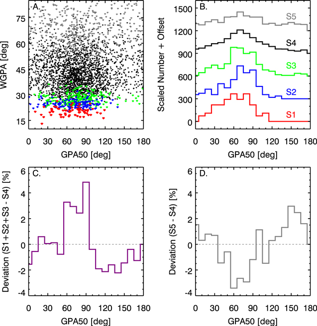
Figure 18. Distributions of median GPA values for GPIPS FOVs. (Upper left, panel A): WGPA vs. GPA50 for all GPIPS FOVs, with symbols representing the S1, S2, S3, S4, and S5 subsamples of FOVs colored red, blue, green, black, and gray, as in Figure 16, respectively. (Upper right, panel B): GPA50 histograms for each of the subsamples of GPIPS FOVs. The histograms have been offset successively by 300 and each non-black histogram was scaled to have the same total FOV counts as in the S4 black histogram, for ease of comparison. (Lower left, panel C): difference histogram, in purple, of scaled S1+S2+S3 (red+green+blue) histograms from panel B minus the S4 (black) FOV histogram. There is an excess of high-P50 FOVs having GPA50 values near 60°–90° and a deficit of intermediate GPA50 values greater than 90°. (Lower right, panel D): difference histogram, in gray, computed from the scaled S5 (gray) histogram of panel B minus the S4 (black) histogram from that panel.
Download figure:
Standard image High-resolution imageTo examine how the various subsamples of FOVs are distributed in GPA50, scaled histograms were formed and are shown as the upper-right panel B in Figure 18. The points in the upper-left panel A were binned by GPA50 separately for each of the subsamples. The resulting histograms were scaled to the same integrated number of FOV counts as in the (typical) S4 sample (black histogram; 2334 FOVs) and successively offset by 300 counts. All five histograms show mostly similar behavior: a broad peak near GPA50 = 75°, with a slow decay to lower GPA50 values and a faster decay to greater GPA50 values. Hence, all GPIPS FOVs appear to be drawn from nearly the same parent GPA50 distribution. However, subtle differences can be seen, especially when comparing the high-P50 S1 (red) and low-P50 S5 (gray) histograms. The high-P50 S1 histogram appears to have a more concentrated peak region and no counts beyond GPA50 = 120°. The low-P50 S5 histogram has a broader peak region and a broader distributed region, with significant FOV counts beyond GPA50 = 120°.
These small differences were enhanced by forming differences of the high-P50 and low-P50 histograms against the average-P50 histogram. The S1 (red), S2 (blue), and S3 (green) histograms were added and scaled to the total FOV counts in the S4 (black) histogram, and these two resulting histograms were differenced to create the purple histogram in the lower-left, panel C of Figure 18. Similarly, the S5 low-P50 histogram (gray) was scaled to the S4 (black) histogram and differenced to create the gray histogram in the lower-right, panel D. In panel C, the high-P/low-WGPA FOVs show an excess of GPIPS FOVs exhibiting near-disk-parallel, 60°–90° GPA50 values, relative to the average GPIPS FOVs, and a deficit of FOVs with GPA50 values in the 110°–170° range. In panel D, the low-P50/high-WGPA, gray difference histogram shows features with almost opposite behavior, showing a broad deficit for GPA50 values in the range 30°–90° and a slight excess of FOVs, relative to the average, for GPA50 values in the 120°–175° range.
The panel-C (purple) and panel-D (gray) difference histograms give the impression of being anticorrelated, but upon plotting the panel-C y-axis values against the panel-D y-axis values and fitting, the linear correlation coefficient was found to be small (−0.67 for 19 points) and not significant. Given the peaked shape of the S4 (black) average FOV sample in panel B, the feature seen in the panel-D (gray) difference histogram likely only indicates that the upper-right, panel B S5 (gray) histogram is wider and flatter than the S4 (black) histogram. Thus, in differencing, that which survives to become the S5–S4 (gray) histogram in panel D is essentially just the negative of the S4 (black) histogram in panel B.
In summary, the strong (or uniform) magnetic field candidate zones, traced by the high-P50/low-WGPA GPIPS FOVs, appear to have a slight preference for exhibiting GPA50 values consistent with magnetic fields that are disk parallel, while the low-P50/high-WGPA GPIPS FOVs appear to have mostly random magnetic field orientations. These properties are somewhat in agreement with the findings reported for Planck polarization data in Planck Collaboration et al. (2015), though no strong evidence is found here for the high-WGPA (weak field) FOVs to be located surrounding the low-WGPA (strong field) FOVs, and the size scales of the high-P50 groups are much smaller than for the Planck-identified regions.
5.3. Remaining Questions
The GPIPS data analyses presented above have revealed new aspects of the nature of the magnetic field in the cold, dusty, star-forming molecular component of the ISM in the disk of the first quadrant of the inner Galaxy. In doing so, questions have arisen about the locations and natures of the newly found structures.
The orientations of NIR polarizations across the GPIPS zone are mostly parallel to the Galactic midplane, but not perfectly so. An overall offset of about 13°–15° is present. Resolved regions show orientations that differ by up to 90° from the Galactic disk orientation. Is the overall offset merely due to contamination by a few regions showing large GPA offsets? What are the natures of those GPA offset regions? How do they relate to star formation zones, supernovae, and/or large-scale outflows off the disk midplane? How would counterparts in external galaxies appear?
How well do magnetic fields follow spiral arms? If material (stars, gas, and dust) flows into and through the arms, how does that affect the spiral magnetic field? Do cool gas and dust clouds acquire magnetic fields in spiral arms, or do they retain magnetic fields established at formation?
Magnetic fields in the Milky Way and external galaxies may be apportioned into large-scale (uniform), medium-scale (anisotropic random), and small-scale (random, tangled, or turbulent) aspects (see reviews by Beck 2015; Haverkorn 2015). What can the wealth of cold-ISM-probing GPIPS data reveal about the natures of the magnetic field on these different size scales in comparison to the corresponding hot-ISM values? What are the mean sizes of magnetically coherent zones or cells (e.g., Jones et al. 1992)? What is the GPIPS-measured ratio of uniform-to-random magnetic field strength, and how does it change with location?
6. Summary
GPIPS was conducted to help reveal the detailed plane-of-sky orientations of the magnetic field in the cool, dusty, star-forming ISM of the disk of the Milky Way in the first Galactic quadrant. GPIPS used near-infrared (NIR) observations in the H band (1.6 μm) to obtain background starlight polarimetry across 76 deg2 of the Galactic midplane. It achieved almost 30'' mean angular sampling for linear polarization measurements.
GPIPS Data Release 4 (DR4) provides H-band in-band stellar magnitudes, linear Stokes parameters, and derived polarization properties as well as 2MASS, GLIMPSE, WISE, and Gaia DR2 cross-references and key data values. GPIPS DR4 contains almost 10 million stellar polarization measurements, of which more than 1 million are of high-enough quality to permit individual use. The remaining almost 9 million will be most useful when considered together in Bayesian or other analysis methods in conjunction with archival photometric, parallax, and spectroscopic data.
Here, the high-quality GPIPS data for each of the 3237 observed 10' × 10' FOVs were converted to distribution functions for four key properties: the number of stars per FOV, the median polarization percentage, the median polarization position angle, and the interquartile range of the position angle distribution. Those FOV-based properties were themselves converted to distribution functions, one-dimensional averages (in each of Galactic longitude and latitude), and two-dimensional distributions of these properties. The median number of high-quality GPIPS stars per FOV is 252, or about 60 per Planck polarization resolution element. Median NIR polarization percentages are around 1.5% for the H band.
The median polarization position angle, in Galactic coordinates (GPA), is about 767, some 133 offset from that expected for a magnetic field oriented parallel to the Galactic disk midplane. While none of the four key characterizing properties showed strong variation with Galactic latitude, longitude variations of GPA were highly significant. Many zones show GPA deviations of 30°–90° from being disk parallel.
Because NIR polarization arises due to alignment of dust grains within dusty molecular clouds, which also introduce significant extinction, there are distance limits imposed on the detection of GPIPS stars, which favor sensing the magnetic field in the portion of the first quadrant closer than about 6–7 kpc. This region includes portions of the Sagittarius and Scutum spiral arms and perhaps the near-side end of the central Galactic Bar. This represents an advantage for GPIPS in being able to accurately reveal the direction of the magnetic field over limited sight-line distances, in comparison to Planck polarimetry, which carries contributions spanning vastly greater distances and thereby misses small-scale and localized changes in magnetic field properties.
An anticorrelation of the median polarization percentages with the widths of the position angle distributions for the FOV-based analysis was revealed and found to be generally similar to that seen in Planck analyses ("S × P": Planck Collaboration et al. 2015, 2018). There are important differences, however. The angular sizes of the 10 largest groups showing high median polarization percentages (and presumably stronger magnetic field strengths) in GPIPS are nearly an order of magnitude smaller than the zones seen in Planck. Also, the suggestion that the high-polarization zones are surrounded by low-polarization shells or membranes (Planck Collaboration et al. 2015) is not supported by analysis of the GPIPS data.
In addition to the authors, GPIPS observations were conducted by S. Hoq, J. Shiode, J. Moreau, M. Bartlett, C. Trombley, and M. Hart. S. Hoq and T. Pillai provided valued manuscript edits and suggested improvements. This research has made use of the VizieR catalog access tool, CDS, Strasbourg, France (doi:10.26093/cds/vizier), originally described in Ochsenbein et al. (2000). GPIPS DR4 includes data from the European Space Agency (ESA) mission Gaia (https://www.cosmos.esa.int/gaia), processed by the Gaia Data Processing and Analysis Consortium (DPAC, https://www.cosmos.esa.int/web/gaia/dpac/consortium). Funding for the DPAC has been provided by national institutions, in particular the institutions participating in the Gaia Multilateral Agreement. GPIPS DR4 also includes data products from the Two Micron All Sky Survey, which is a joint project of the University of Massachusetts and the Infrared Processing and Analysis Center/California Institute of Technology, funded by NASA and NSF. This publication makes use of data products from the Wide-Field Infrared Survey Explorer, which is a joint project of the University of California, Los Angeles, and the Jet Propulsion Laboratory (JPL)/California Institute of Technology (CalTech), funded by NASA. This work is based in part on observations made with the Spitzer Space Telescope, which was operated by JPL/CalTech under a contract with NASA. This research was conducted using the Mimir instrument, jointly developed at Boston University and Lowell Observatory and supported by NASA, NSF, and the W.M. Keck Foundation. Massachusetts NASA Space Grant number 165283 from MIT to Boston University partially supported C.C. during 2018 summer and is gratefully acknowledged. The GPIPS effort has been made possible by grants AST 06-07500, 09-07790, 14-12269, and 18-14531 from NSF/MPS to Boston University and by grants of significant observing time (BU key project status) from the Boston University—Lowell Observatory partnership.
Facility: Perkins. -
Appendix A: Data Quality Evaluations
Checks and evaluations of data obtained for GPIPS were performed as the data were collected, reduced, and analyzed to develop provisional data products. Observations judged to have not met the quality standards described below were rejected, and the FOV(s) was (were) reobserved as needed to obtain the high-quality data required for inclusion in the final GPIPS DR4 data products.
Table A1 presents a shortened, representative portion of the Field Properties Summary Table, which is contained in the full DR4 file set. The FOV rows selected for presentation in Table A1 highlight FOVs that passed all of the quality controls and a couple of FOVs that did not fully meet one quality test. In the table, the first column lists the sequential GPIPS FOV number, from 0001 to 3237. The second and third columns list the Galactic coordinates of the true centers of the observed FOVs. Note that all image orientations were equatorial. The fourth column lists the angular offset, in arcsecond, of the true FOV center direction from the nominal GPIPS grid center direction. Adjacent GPIPS grid centers were designed to provide FOV overlap by up to 1', so acceptable offset values were generally less than about 45''. The largest center position offset that was judged acceptable was 55''. The fifth column lists the observing night designations, in YYYYMMDD form of the UT date. The sixth column identifies the first image number of the observation and may be matched to the handwritten observing logs (available from the DR4 website) to obtain sky and instrument context regarding specific observations. The seventh column lists the FWHM of the deep photometric image PSF, in arcseconds, corrected for the pixel sampling contribution.
Table A1. GPIPS Field Properties Summary Table
| GPIPS | Galactic | Galactic | Center | UT | First | PSF | Secular | Sky | Rejected | Accepted | Pattern | QC |
|---|---|---|---|---|---|---|---|---|---|---|---|---|
| FOV | Long. | Lat. | Offset | Night Desig. | Image | FWHM | Ampl. | Noise | Image | Image | Score | Flag |
| No. | (deg) | (deg) | (arcsec) | (Y4M2D2) | No. | (arcsec) | (%) | (%) | Count | Count | ||
| (1) | (2) | (3) | (4) | (5) | (6) | (7) | (8) | (9) | (10) | (11) | (12) | (13) |
| 0001 | 18.082 | −0.635 | 5.5 | 20070919 | 316 | 1.196 | 1.0 | 0.61 | 6 | 96 | 6 | 0 |
| 0002 | 18.151 | −0.767 | 6.1 | 20080608 | 2232 | 1.265 | 0.0 | 0.34 | 2 | 99 | 5 | 0 |
| ... | ||||||||||||
| 0460 | 23.005 | 0.949 | 32.7 | 20120614 | 2892 | 1.853 | 0.0 | 0.55 | 0 | 96 | 4 | 0 |
| 0461 | 23.078 | 0.826 | 2.4 | 20190627 | 1329 | 1.299 | 0.7 | 0.35 | 0 | 96 | 0 | 2 |
| 0462 | 23.143 | 0.690 | 15.1 | 20110609 | 2757 | 1.786 | 0.0 | 0.40 | 0 | 96 | 7 | 0 |
| ... | ||||||||||||
| 3128 | 54.851 | −0.381 | 10.8 | 20100605 | 1290 | 1.609 | 0.5 | 0.39 | 0 | 102 | 4 | 0 |
| 3129 | 54.924 | −0.514 | 6.9 | 20130626 | 1105 | 1.485 | 0.0 | 0.45 | 1 | 95 | 1 | 1 |
| 3130 | 54.999 | −0.646 | 1.6 | 20170527 | 1745 | 1.658 | 0.8 | 0.53 | 0 | 96 | 9 | 0 |
Note. This is a shortened and selective portion of the full table that is available on the GPIPS DR4 website (http://sites.bu.edu/gpips).
Only a portion of this table is shown here to demonstrate its form and content. A machine-readable version of the full table is available.
Download table as: DataTypeset image
Column eight lists the secular amplitude for each observation. This represents the slow variation in stellar brightness levels (above the background sky) for the typically ∼300 bright stars per FOV matched between the first image and each of the remaining 95–118 images for an observation (e.g., Figure 10 of Paper I). Secular amplitude values exceeding 3% were judged to indicate contamination by clouds or other problems, and those FOVs were reobserved. The ninth column lists the amplitude of the sky noise, computed as the rms of the image-to-image star-matched brightness changes, after removal of the secular variation and removal of the modulation by the average polarization for the FOV. This characterization is also described in detail in Appendix B of Paper I. Sky-noise levels above 1.2% were judged excessive, and those FOVs were reobserved. Of the 3237 FOVs, only one FOV exceeded this criterion and was retained (its sky-noise value was 1.3%). The number of images rejected from each observation set for poor PSF shapes is listed in column 10. At least 89 acceptable images per FOV were required for an observation to be included, and the number of accepted images is listed in column 11. This criterion ensured that multiple images would sample all 16 HWP orientation angles.
Column 12 lists a pattern score for each FOV. These were formed by combining seven different quantitative evaluations of the polarization percentage and orientation patterns for each FOV. They were used to assess whether the resulting polarization patterns resembled parallel orientation directions or orientation directions that aligned tangentially (i.e., swirls), if the polarization percentage increased with offset from the image center, and other negative characteristics. These evaluations uncovered several observing or data reduction failures, including cases of frozen HWP rotation, bad flat-field images, and other issues. A custom software tool, coded in IDL, was created to view the polarization pattern for each FOV observing set and to apply the seven evaluations. These component scores were combined to be the pattern score, scaled to range from −9 to +9.
Strongly negative pattern scores correlated with nonphysical, swirl-like orientation patterns that also had polarization percentages rising with radial offset from image centers, neither of which should occur. Strongly positive pattern scores showed highly parallel polarization orientations and an absence of data problems. Score values less than zero indicated possible problems, and those FOVs were reobserved. Some FOVs exhibited complex polarization orientation patterns resulting in midrange, but mostly positive, pattern scores. Reobservation of many of these FOVs recovered the same complex polarization patterns, reinforcing their veracity. First reobservations of negative-scoring FOVs generally did not yield polarization patterns consistent with the initial observations, so these FOVs were reobserved until the patterns became stable in subsequent observations, which resulted in their pattern scores becoming positive.
The final column in the table contains a quality control (QC) flag to indicate the overall quality of the final data for each observed FOV. In this column, a zero entry means the observation met all of the criteria for PSF quality, secular amplitude, sky noise, good image count, and polarization pattern score. Values greater than zero represent weighted degrees of departure from the goals. Of the 3237 FOVs comprising GPIPS, 3145 (97.2%) met all of the quality goals, and so have zero-value entries in the QC flag column. Three FOVs had QC flag values of 2 (field numbers 461 (listed in Table A1), 487, and 2115) due to their pattern scores being 0. Eighty-two FOVs had QC values of unity, including FOV number 3129, which is also listed in Table A1. All of these are due to their pattern scores being unity, that is, weakly positive but not as strongly positive (exhibiting highly parallel polarization orientations) as for other fields. Six of the remaining seven FOVs with unity QC values showed moderately higher secular amplitudes and center position offsets.
Appendix B: Matching Gaia DR2, 2MASS, GLIMPSE, and WISE Stars to GPIPS Stars
Stellar data for archival Gaia DR2, 2MASS, GLIMPSE, and WISE catalog entries were fetched using the VizieR catalog tool (Ochsenbein et al. 2000) for all point sources contained within the boundaries of each GPIPS FOV, using searches centered at the actual observed coordinates (Table A1). Because GPIPS observations were obtained using sky dithering, with later sky registration and coadding of the images, the resulting deep photometric and HWP images do not have sharply defined uniform exposure edges nor uniform sizes. To set the search area for each FOV, the PHOTCAT stars with the least and greatest R.A. and decl. values in the FOV were used to delineate the search box extent. To this, an additional 15 wide outer zone was added to extend the field sizes to provide some margin for individual star matching, as described below. The resulting search field sizes averaged about 99 × 99, somewhat smaller than the Mimir instrument FOV. The effective field size for the archival catalog searches is about 1% larger than the effective DR4 FOV size (see Section 3.2), which should bias the matching statistics only slightly.
Archival stars were matched to GPIPS stars in each FOV for each of the four catalogs using cone searches with maximum relative projected radial offsets of 125 between GPIPS stars and archival catalog stars. This value was selected based on using matches of test FOVs employing a set of trial cone angle values. Star matching was performed starting from the brightest to the faintest GPIPS stars in each FOV, and similarly brightest to faintest archival catalog stars, to minimize false matches that might have resulted from the large numbers of faint stars. A few GPIPS stars were found to have potential matches to multiple archival catalog stars within the radial offset limit. For these cases, color values were computed for each star (e.g., Gaia g band minus Mimir H band) and were combined with the radial offset values using Gaussian probability functions to select the single most likely stellar match. Stars, once matched, were removed from the remaining GPIPS and archival catalog potential matching pools.
B.1. Match Rates
Table B1 provides summaries of the numbers and rates of stellar matches of archival catalogs to GPIPS. Additionally, for the POLCAT stars, the matching numbers and fractions for each of the UF1 (and its UF0 subset, listed in italics), UF2, and UF3 star subsets are indicated. Using Table B1, reverse match rates, for example, the fraction of Gaia stars that have GPIPS POLCAT UF1 matches, may be computed from the match numbers divided by the total entries for each of the four archival catalogs across the GPIPS FOVs. These totals are listed in the final row of Table B1.
Table B1. Match Properties for GPIPS Stars Found in Archival Catalogs
| GPIPS | Gaia DR2 | 2MASS | GLIMPSE | WISE | |
|---|---|---|---|---|---|
| Data Set | All | Parallax | |||
| (1) | (2) | (3) | (4) | (5) | (6) |
| PHOTCAT | 7,740,701 | 5,054,289 | 8,350,602 | 10,955,641 | 1,702,876 |
| 49.9% | 32.6% | 53.8% | 70.6% | 11.0% | |
| POLCAT | 5,641,339 | 3,839,159 | 7,219,367 | 8,361,968 | 1,657,927 |
| 58.1% | 39.5% | 74.4% | 86.1% | 17.1% | |
| UF1 | 857,887 | 638,523 | 985,415 | 1,011,415 | 721,267 |
| 84.0% | 62.5% | 96.5% | 99.0% | 70.6% | |
| UF0 | 180,951 | 128,453 | 234,215 | 237,449 | 208,154 |
| 75.7% | 53.8% | 98.0% | 99.4% | 87.1% | |
| UF2 | 1,916,938 | 1,273,736 | 2,504,421 | 2,691,718 | 674,206 |
| 66.6% | 44.3% | 87.1% | 93.6% | 23.4% | |
| UF3 | 2,866,514 | 1,926,900 | 3,729,531 | 4,658,835 | 262,454 |
| 49.3% | 33.2% | 64.2% | 80.2% | 4.5% | |
| Archival Totals | 13,884,329 | 7,753,503 | 9,198,385 | 18,331,898 | 2,109,578 |
Download table as: ASCIITypeset image
The greatest match rates of GPIPS to archival catalogs occurs for GLIMPSE. The lowest GLIMPSE match rate is 70.6% for PHOTCATs and the highest is 99.4% for the UF0 subset of UF1 GPIPS stars. For every UF stellar category, the rate of matching to GLIMPSE stars is higher than it is to any of the other three archival catalogs. This is a distinct improvement compared to the GPIPS DR1 matching approach and offers the opportunity to use the H band from GPIPS and the M-band equivalent (4.5 μm) from GLIMPSE to quantify the line-of-sight extinction using the (H − M) colors with the Rayleigh–Jeans color excess method (RJCE; Majewski et al. 2011).
In Table B1, the Gaia DR2 columns report the matching stellar numbers and rates for GPIPS stars for the case of no application of the parallax evaluation (the "All" column) and for matching to stars with the potentially useful parallax criteria (the "Parallax" column).
Overall, GPIPS POLCAT match rates with the archival catalogs are somewhat greater than the PHOTCAT ones, as the latter contains more faint stars than the former. The overall GPIPS POLCAT match rates are about 58% for Gaia (40% for Gaia stars with parallaxes), 74% for 2MASS, 86% for GLIMPSE, and 17% for WISE. WISE is generally more sensitive than the Spitzer Infrared Array Camera (IRAC; Fazio et al. 2004), used to conduct the GLIMPSE observations, for directions away from the Galactic plane. But, WISE has coarser angular resolution than IRAC, resulting in a brighter confusion limit in the Galactic plane and fewer sources per GPIPS FOV than for GLIMPSE in the same wave bands.
In Table B1, there is a trend of increasing GPIPS match rates as UF number decreases, corresponding to increasing apparent brightness. The one interesting exception is the POLCAT UF0 subset matching to Gaia, which shows somewhat lower rates than the larger UF1 sample which contains UF0. This could be caused by the greater P' values in UF0 arising because of their greater dust column densities and thereby greater AV values. This in turn would affect Gaia matches through the optical g-band brightness limit, as these shorter wavelengths would suffer the greatest extinctions.
The archival catalog matching information was integrated into GPIPS in two ways, one related to the FOV-based data products and one related to the unique star data file.
B.2. FOV-based Archival Catalog Stellar Match Data Files
For the FOV-based products, the 2MASS and GLIMPSE matching stellar information was directly integrated into the PHOTCAT and POLCAT files for each of the 3237 GPIPS FOVs. These 2MASS and GLIMPSE values supersede the values listed in the GPIPS DR1 through DR3 listings, as follows. Prior to DR4, only the highest-quality 2MASS data were included in GPIPS files by requiring an "A" photometry quality rating for each of the J-, H-, and K-band 2MASS magnitudes (Skrutskie et al. 2006). For DR4, this criterion was removed, allowing all 2MASS matches to be included. The fraction of GPIPS POLCAT stars with 2MASS entries thereby increased from about 64% for DR1 to about 74% for DR4. Similarly, prior to DR4, GLIMPSE data were included in GPIPS files only through being matched via their 2MASS designations. For DR4, GLIMPSE point-source positions were directly matched to GPIPS stars and were included in GPIPS files. This approach greatly increased the fraction of GPIPS entries with GLIMPSE matches, especially those for which 2MASS matches were lacking due to faintness.
The Gaia DR2 stellar data were further examined to determine the quality of the parallax information provided in DR2. Stars with possibly useful parallax values for GPIPS applications by potential users were judged to be those for which the parallax S/N (π/σπ) was greater than 0.5 and the parallax value was greater than −2 mas. As noted earlier in the text, these liberal limits will mainly remove nondetection upper limits and spurious values while avoiding potential population biases (Bailer-Jones et al. 2018; Luri et al. 2018). These do not include the additional criteria on g-band magnitude, H-band magnitude, or (H – K) color uncertainties that were applied to create Figures 2–4 and the associated summaries presented in Table 2.
For each of Gaia DR2, 2MASS, GLIMPSE, and WISE, the FOV-based approach generated one data file per FOV for each of these four archival catalogs. In each file, every archival star contained within the FOV search area for that catalog is listed, along with PHOTCAT and POLCAT star identifiers for each matching GPIPS star. This approach provides bidirectional matching information and enables characterizing match success rates. Note that these match rates are somewhat optimistic, in the sense that not every match of an archival star to a GPIPS star will necessarily provide uniformly high-quality stellar information. Users are strongly encouraged to evaluate the uncertainties listed for each reported value for matches between GPIPS and the archival entries.
Each Gaia, 2MASS, GLIMPSE, and WISE match file has metadata for the GPIPS FOV number, search center sky direction in R.A. and decl., and field search size in the R.A. and decl. directions. Each match file has one row for each archival star found in the search field. Each lists an R.A.-ordered star number, followed by entries listing the matching POLCAT and/or PHOTCAT star, referenced to the identifying entries in the GPIPS files, or a −99 value to indicate no match to a GPIPS star was found. The R.A. and decl. listed in the archival catalog follow next. The 2MASS, GLIMPSE, and WISE match file rows next list the three- or four-band magnitudes and uncertainties (J, H, and K for 2MASS; 3.6, 4.5, 5.8, and 8.0 μm for GLIMPSE; W1[3.6], W2[4.5], W3[12], and W4[22 μm] for WISE), followed by the star designation unique to that catalog.
Gaia DR2 match files contain similar metadata, star numbers, GPIPS star numbers, and R.A. and decl. values as reported in Gaia DR2. Next, each row lists the Gaia g-band magnitude, g-band magnitude uncertainty, parallax, parallax uncertainty, proper motions and their uncertainties in the R.A. and decl. directions, and the Gaia star designation label.
B.3. Unique Star Data File Contents and Archival Match Information
As an alternative to the FOV-based data files, the unique star data file (Clemens et al. 2020) collects all GPIPS photometry and polarimetry and all matching stellar data appropriate to each GPIPS star, with data fields for each star as listed in the example entry shown as Table B2. The unique star file contains entries for 13,861,329 GPIPS stars found in the 3237 PHOTCAT files.
Table B2. Data Fields for Each Star in the Unique Star File
| Field Name | Type | Example Values | Description |
|---|---|---|---|
| NUM | La | 605776 | R.A.-ordered star serial number |
| DESIG_GPIPS | S | "GPIPS_J182558.20-124843.5" | |
| RA_DEG | D | 276.49249 | J2000 R.A., in degrees |
| DEC_DEG | D | −12.81209 | J2000 decl., in degrees |
| GAL_L | D | 18.65135 | Galactic longitude, in degrees |
| GAL_B | D | −0.27934 | Galactic latitude, in degrees |
| GPSTAR | L | Array[4]: | FOV × 105 + stellar ID No. |
| L | 3405524 | Observation 1: FOV 34, star number 5524 | |
| L | 3500495 | Observation 2: FOV 35, star number 495 | |
| L | 4806180 | Observation 3: FOV 48, star number 180 | |
| L | 4900307 | Observation 4: FOV 49, star number 307 | |
| CAT_FLAG | I | Array[5]: | Array of archive catalog match codes |
| I | 1 | a POLCAT star matched, if = 1 | |
| I | 31 | a Gaia DR2 star matched, see Table B3 for code meaning | |
| I | 7 | a 2MASS star matched, see Table B3 for code meaning | |
| I | 15 | a GLIMPSE star matched, see Table B3 for code meaning | |
| I | 31 | a WISE star matched, see Table B3 for code meaning | |
| H_MAG | D | 10.31231 | Mimir H-band photometric magnitude |
| E_HMAG | D | 0.00039 | Internal uncertainty in H-band mag. |
| S_PHOT | D | 0.02254 | External H-band mag. uncert. (see Clemens et al. 2012a) |
| H_VAR | I | 0 | Variability flag for overlapping FOVs (see text) |
| P | D | 1.47 | Debiased polarization percentage (P') |
| E_P | D | 0.33 | Uncertainty in polarization percentage |
| PA_DEG | D | 13.7 | Polarization position angle (EPA) E of N, in degrees |
| GPA_DEG | D | 75.9 | Galactic position angle (GPA), in degrees |
| E_PA | D | 6.3 | Uncertainty in position angles, in degrees |
| Q | D | 1.34 | Stokes Q (%), normalized by Stokes I |
| E_Q | D | 0.33 | Uncertainty in Stokes Q (%) |
| U | D | 0.69 | Stokes U (%), normalized by Stokes I |
| E_U | D | 0.32 | Uncertainty in Stokes U (%) |
| NHWP | I | 64 | Number of HWP images in which the star appears (see text) |
| UF | I | 1 | Usage Flag (1, 2, 3, or −99) (Clemens et al. 2012a) |
| Designations in Archival Catalogs | |||
| DESIG_GAIA | S | "Gaia DR2 4152582674817733760" | |
| DESIG_2MASS | S | "J18255820-1248437" | |
| DESIG_GLIMPSE | S | "G018.6514-00.2794" | |
| DESIG_WISE | S | "J182558.18-124842.9" | |
| Gaia DR2 data values: | |||
| PAR | D | 0.0056 | Parallax, in milliarcseconds |
| E_PAR | D | 0.1948 | Uncertainty in parallax, in milliarcseconds |
| GMAG | D | 17.1452 | g-band photometric magnitude |
| E_GMAG | D | 0.0016 | Uncertainty in g-band magnitude |
| PMRA | D | 0.128 | Proper motion along R.A., in mas yr−1 |
| E_PMRA | D | 0.329 | Uncertainty in R.A. proper motion, in mas yr−1 |
| PMDEC | D | −2.088 | Proper motion along decl., in mas yr−1 |
| E_PMDEC | D | 0.372 | Uncertainty in decl. proper motion, in mas yr−1 |
| 2MASS data values: | |||
| J_2MASS | D | 11.975 | J-band photometric magnitude |
| E_J2MASS | D | 0.033 | Uncertainty in J-band mag |
| H_2MASS | D | 10.408 | H-band photometric magnitude |
| E_H2MASS | D | 0.058 | Uncertainty in H-band magnitude |
| K_2MASS | D | 9.784 | K-band photometric magnitude |
| E_K2MASS | D | 99.99 | Uncertainty in K-band magnitude (note upper limit) |
| GLIMPSE data values: | |||
| B36MAG | D | 9.137 | IRAC 3.6 μm ("∼L") band photometric magnitude |
| E_B36MAG | D | 0.104 | Uncertainty in IRAC 3.6 μm band magnitude |
| B45MAG | D | 9.011 | IRAC 4.5 μm ("∼M") band photometric magnitude |
| E_B45MAG | D | 0.078 | Uncertainty in 4.5 μm band magnitude |
| B58MAG | D | 8.795 | IRAC 5.8 μm band photometric magnitude |
| E_B58MAG | D | 0.053 | Uncertainty in IRAC 5.8 μm band magnitude |
| B80MAG | D | 8.767 | IRAC 8.0 μm band photometric magnitude |
| E_B80MAG | D | 99.99 | Uncertainty in IRAC 8.0 μm band magnitude (note upper limit) |
| WISE data values: | |||
| W1MAG | D | 8.975 | WISE band 1 (3.4 μm; "∼L") photometric magnitude |
| E_W1MAG | D | 0.025 | Uncertainty in WISE band 1 magnitude |
| W2MAG | D | 8.877 | WISE band 2 (4.6 μm; "∼M") photometric magnitude |
| E_W2MAG | D | 0.022 | Uncertainty in WISE band 2 magnitude |
| W3MAG | D | 7.733 | WISE band 3 (12 μm) photometric magnitude |
| E_W3MAG | D | 0.195 | Uncertainty in WISE band 3 magnitude |
| W4MAG | D | 3.969 | WISE band 4 (22 μm) photometric magnitude |
| E_W4MAG | D | 0.069 | Uncertainty in WISE band 4 magnitude |
Note.
aData type: I—short integer; L—long integer; D—double precision real; S—string. Arrays are indicated by variable type and number of entries.Most of the data fields in the unique star file are conventional and are based on existing GPIPS Paper III, 2MASS, GLIMPSE, Gaia DR2, and WISE catalogs and can be interpreted using Tables B2 and B3 as guides. Where no data exist or there were no matching archival catalog data, values and/or uncertainties of 99.99 were entered. Where the uncertainty in polarization percentage σP was greater than the raw polarization percentage PRAW, the tabulated polarization percentage ("P" representing debiased P' values) was set to zero, and the corresponding position angle uncertainty SPA was set to 180°. For Gaia matches, upper limits on parallax and proper motions are noted with values of 30.0 and uncertainties of 90.0.
Table B3. CAT_FLAG Entry Encoding
| Entry | Additive | |
|---|---|---|
| Number | Score | Description |
| (1) | (2) | (3) |
| 1 | 1 | GPIPS POLCAT star was matched |
| 2 | 1 | Gaia DR2 star was matched |
| 2 | E_PAR not upper limit (90.0) | |
| 4 | E_GMAG not upper limit (99.99) | |
| 8 | E_PMRA not upper limit (90.0) | |
| 16 | E_PMDEC not upper limit (90.0) | |
| 3 | 1 | 2MASS PSC star was matched |
| 2 | E_J2MASS not upper limit (99.99) | |
| 4 | E_H2MASS not upper limit (99.99) | |
| 8 | E_K2MASS not upper limit (99.99) | |
| 4 | 1 | GLIMPSE star was matched |
| 2 | E_B36MAG not upper limit (99.99) | |
| 4 | E_B45MAG not upper limit (99.99) | |
| 8 | E_B58MAG not upper limit (99.99) | |
| 16 | E_B80MAG not upper limit (99.99) | |
| 5 | 1 | WISE star was matched |
| 2 | E_W1MAG not upper limit (99.99) | |
| 4 | E_W2MAG not upper limit (99.99) | |
| 8 | E_W3MAG not upper limit (99.99) | |
| 16 | E_W4MAG not upper limit (99.99) |
Download table as: ASCIITypeset image
A few of the fields listed in the unique star file are newly introduced here and warrant discussion. The GPSTAR array carries the combined FOV and star number in that FOV for the up to four observations of any one unique star. For the example star shown in Table B2, there were four observations of this star, as indicated in the GPSTAR entries. For stars with only a single observation, the first entry of GPSTAR contains the FOV and star number and the remaining GPSTAR entries are set to −1.
The CAT_FLAG array provides a quick encoding of information regarding the natures of the other catalog properties for stars matched to the unique GPIPS star. The first CAT_FLAG entry is either unity, if there is matching GPIPS polarization information from one or more POLCATs, or zero if there is no POLCAT information for this unique PHOTCAT star. The second through fifth entries encode quality information related to each archival catalog match star, as listed in Table B3. The score codes in the second column of Table B3 were summed for each catalog to create the reported value. That is, a CAT_FLAG score of 31 in the second array entry identifies a Gaia DR2 matched star with reported values of parallax, g-band magnitude, as well as R.A. and decl. values of proper motion. Note that these scores do not indicate confidence levels: instead, they only report the presence or absence of key quantities. Score maxima are unity for GPIPS POLCAT, 15 for 2MASS, and 31 for the remaining catalogs. The CAT_FLAG encoding is not perfect, however. For the example UF1 star values presented in Table B2, the 2MASS K-band and GLIMPSE 8.0 μm band uncertainties are reported as upper limits (with values of 99.99 in their uncertainty fields) while their photometric values are still listed in those archival catalogs as well as here. Users are warned that the quick summaries provided in the CAT_FLAG array may miss such details.
The H_VAR field identifies stars with multiple GPIPS observations that exhibit H-band photometric differences in excess of 10 times their propagated external photometric difference uncertainties. For the up to four observations possible for stars in overlapping FOVs, if any of the (up to) six possible pairwise photometric differences exceed this 10σ threshold then the H_VAR field was set to unity, otherwise it was set to zero. A total of 18,499 stars have H_VAR = 1 values.
In Table B2, the NHWP field most often lists the number of distinct HWP images (up to 16) in which a non-overlapping star was detected. Faint stars might fail to be detected in all 16 HWP images for an FOV, so this field can be useful for culling faint polarization candidates. For overlapping FOVs, NHWP carries the sum of all constituent HWP detection counts, resulting in a maximum value for this field of 64, as is the case for the example star properties listed in Table B2. For stars with PHOTCAT magnitudes but no PHOTCAT matches, the NHWP fields were set to 99. Combining the GPSTAR and NHWP field information will provide adequate insight into whether a multiply observed star was detected in sufficient HWP images to be useful.
Finally, the UF field carries the values 1, 2, or 3 associated with the UF1, UF2, and UF3 classifications described in the text. Note that for multiply observed stars, this classification was reassessed after the stellar polarization data were merged from the multiple observation values. This could result in a lower UF value than appear in the FOV-based single observations of the star. Also, for stars in the PHOTCAT-based unique star file that do not have GPIPS polarization data (e.g., no POLCAT star matches), the UF field was set to −99.
Two potentially useful classes of data are absent in this combined data file. The first is the detailed photometric and polarimetric information obtained for the duplicate stars that appear in more than one GPIPS FOV because of the overlapping nature of the survey. The polarization information for these stars is merged, as described below, in the unique star file, though FOV-identifying information for each merged star is in the GPSTAR array. The second class of missing data are the FOV-based files of archival data, especially of the archival stars in those files that are not matched to GPIPS stars. These unmatched stars are fully absent in the unique star file and are only listed in the FOV-based files. A less vital third class of missing information involves some of the ancillary polarization information, such as where each star appears on the Mimir detector FOV, which is used for instrumental polarization correction. Any later recalibration of the GPIPS polarization, resulting from updated instrumental polarization corrections, will need to utilize the FOV-based POLCATs and/or to rebuild the unique star file. The fourth, minor, missing element is the metadata for each GPIPS FOV, normally included in the PHOTCATs and POLCATs and supported by electronic copies of the handwritten observing logs. The GPSTAR array entries provide information about the original FOVs and star numbers in the constituent observations so that these data may be referenced in the FOV-based data products if needed.
Despite these absences, the DR4 unique star data product is potentially the most useful for accessing GPIPS, as it contains virtually all relevant photometric, polarimetric, and parallax data for conducting a wide variety of studies with the least data-accessing software overhead.
Appendix C: Polarization Signal-to-noise Choices and Effects
In Figures 1 through 5, the UF designations introduced in Paper III are seen to reveal important aspects about the nature of these designated stars and the ISM they probe. One aspect of a uniform survey, such as GPIPS, being applied to a wide range of stellar brightnesses is that there is a nearly continuous and wide range of resulting linear polarization S/Ns present in the sample of stars. Which ratio values to include and which to reject for a particular scientific study depends on the goals and questions posed. For the purposes of this paper, and its primarily FOV-based median polarization (and magnetic field) characterizations, what is the best balance between the number of stars selected for analysis and the signal-to-noise criterion applied to select them that will also accurately reveal the properties of the magnetic field being surveyed?
The UF2 and UF3 classified stars were previously (Paper III) shown to be generally unsuitable as individual probes of plane-of-sky magnetic field properties, though they could serve such purposes with suitable sample or area averaging. Addressed here is the question of whether the UF1 stars are suitable or whether additional, more stringent, signal-to-noise criteria must be applied in order to extract meaningful magnetic field properties from the GPIPS data.
In the following subsections, the UF1 and UF0 polarization properties for the GPIPS-1619 field are compared, the polarization signal-to-noise distributions for all GPIPS stars are considered, and differences between UF1 and UF0 WGPA (see Section 4.2.2) properties are examined for all GPIPS FOVs as functions of the numbers of stars in each FOV as well as the P50 and WGPA values in each field. The conclusion from this examination is that the UF1 stars, those with mH < 12.5 mag and σP < 2%, are shown to reveal magnetic field properties in the GPIPS-1619 field nearly as well as their UF0 subset. Also, consideration of the full set of GPIPS FOVs does not change this conclusion.
C.1. GPIPS-1619 Comparisons
Figure C1 presents the same histograms of P' and GPA for the UF1 stars found in the GPIPS-1619 FOV as was previously displayed as Figure 6, but here adds histograms in yellow for the UF0 stars that additionally meet a P'S/N ≥ 3 criterion. Analysis of the UF0 histograms yields P' quartile boundaries of 1.76%, 2.57%, and 3.73% and GPA quartile boundaries of 865, 992, and 1116, which are indicated as vertical, dashed, yellow lines at the quartile locations. These UF0 star polarization properties do not differ greatly from those derived from the larger UF1 set, though the UF0 P' values are biased to greater values through rejection of lower polarization percentages.

Figure C1. Histograms of debiased polarization percentage P' (left, panel A) and Galactic position angle GPA (right, panel B) for UF1 stars (red lines) and UF0 stars (those with P'S/N ≥ 3; yellow lines) in GPIPS-1619 (previously shown as Figure 6 for the UF1 stars only). These histograms were constructed using accumulated Gaussian distribution representations for the properties of each star. Cumulative probability distributions for the UF1 stars are shown as the smooth red curves that connect points centered in each bin and are referenced to the right axis labels. Vertical red dashed lines and labels identify the locations of the three quartile boundaries of the cumulative distributions for the UF1 stars. The similar quartile boundaries for the UF0 stars are shown as the vertical dashed yellow lines.
Download figure:
Standard image High-resolution imageC.2. Polarization Signal-to-noise Distribution Properties
Figure C2(A) (top panel) shows histograms of all POLCAT stars as a function of raw (not debiased) polarization signal to noise (PS/N ≡ PRAW/σP) for the UF1, UF2, and UF3 subsets and for all GPIPS stars, as red, blue, green, and black curves, respectively. Figure C2(B) (lower panel) shows their cumulative distributions. Vertical dashed gray lines indicate where PRAW/σP is unity. When their raw polarization values are debiased to become P', all stars to the left of the unity lines would become polarization upper limits. Hence, the PRAW/σP distributions capture better the full range of GPIPS data quality than would the debiased (P' S/N) distributions.
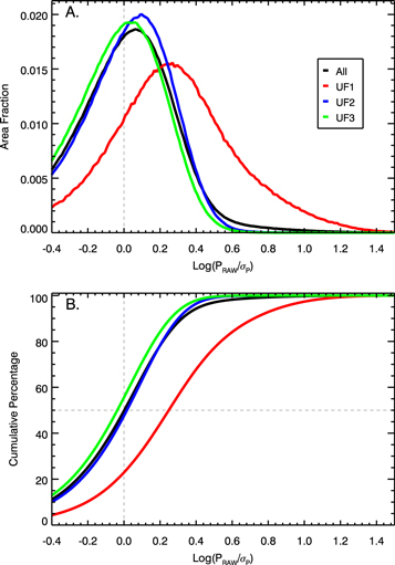
Figure C2. Raw polarization percentage signal-to-noise ratio (PS/N ≡ PRAW/σP) distributions of GPIPS POLCAT stars. Horizontal axes show the base10 logarithm of PS/N. (Top, panel A) Distributions of PS/N by UF classification subset. The vertical axis is the fractional probability for each GPIPS UF data subset. The distribution of PS/N for the combination of all GPIPS POLCAT stars is plotted in black. The UF1 distribution is shown in red. The UF2 and UF3 distributions are shown in blue and green, respectively. The vertical dashed line represents unity PS/N. (Bottom, panel B) Cumulative PS/N distributions, with the same mapping of UF subset type to color. While the UF2 and UF3 stars show median PS/N values near unity, and thus are expected to exhibit strong noise bias, the UF1 stars are dominated by significant PS/N ratios.
Download figure:
Standard image High-resolution imageIn Figure C2(A), the UF2, UF3, and combined ("All") GPIPS distributions exhibit peaks that are located somewhat to the right of the PS/N unity line. Their cumulative distributions (panel B) show that their median values are also close to unity PRAW/σP. That the combined GPIPS distribution follows closely the UF2 and UF3 distributions is because those subsamples dominate in numbers of stars over the UF1 sample (90% versus 10%). The UF1 histogram, however, is shifted to higher PS/N values. Its cumulative distribution (panel B) shows that 20% of UF1 stars have PRAW/σP of unity or less and 80% of the UF1 stars show PRAW/σP in excess of unity.
C.3. Effects of Different P'S/N Selections
Next, a sweep of P'S/N criterion choices was performed for the GPIPS-1619 FOV stellar data, followed by a limited comparison of results for two P'S/N criterion choices for the full set of GPIPS FOVs. The evaluating quantity was the interquartile range WGPA, selected as likely the most sensitive to changes in the nature of the polarization properties of the different stellar subsamples.
For the GPIPS-1619 examination, subsets were drawn from the UF1 stars, applying additional P'S/N criteria that stepped from zero through the UF0 value of three and on to five. The resulting run of WGPA versus P'S/N for the GP1619 FOV is presented in Figure C3. In the figure, the blue diamonds and blue connecting lines show the decrease in WGPA values as P'S/N is increased. The red triangles and connecting lines show the numbers of stars meeting the P'S/N criteria. Both curves fall with increasing P'S/N, as fewer stars in the GPIPS-1619 FOV meet the selection criterion. The overall decrease in WGPA, with P'S/N ranging from zero to five, is about 32% for this FOV while the number of stars decreases by 70%. The lower WGPA values might signal greater coherence of the magnetic field in the plane of the sky, but the associated lower star numbers could also be suggesting the introduction of a bias due to, for example, the selected stars only sampling higher-extinction lines of sight. Such lines of sight could be limited to only a small, dusty region within the FOV and not representative of the magnetic field properties across the full FOV.
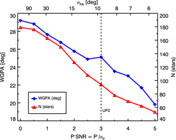
Figure C3. Interquartile ranges of WGPA, and the numbers of selected stars, vs. debiased polarization percentage signal-to-noise P'S/N for stars in the GPIPS-1619 FOV. WGPA values, computed for P'S/N lower limits stepped by 0.5 from zero, are shown as blue diamonds connected by blue line segments and are referenced to the left vertical axis. The numbers of stars in the GPIPS-1619 FOV meeting each P'S/N cutoff are shown as the red triangles connected by red line segments and are referenced to the right vertical axis. The top horizontal axis indicate polarization position angle uncertainties computed from the P'S/N limits shown in the bottom axis.
Download figure:
Standard image High-resolution imageTo uncover the nature of possible biases introduced by the addition of a P'S/N criterion to the UF1 selection criteria, a representative ratio R was developed. It was computed from the ratio of the WGPA value found when selecting a stellar subsample of UF1 stars using the UF0 criterion (P'S/N ≥ 3) to the WGPA value for the UF1 stars alone (e.g., R ≡ WGPAUF0/WGPAUF1). Figure C4(A) (upper left) shows the histogram of R values obtained for the set of all 3237 GPIPS FOVs. There is a well-defined peak, near the median, with a mean of 0.66 and standard deviation of 0.12. Figure C4(B) (upper right) shows the run of R values with the log of the number of UF1 stars in each GPIPS FOV. No trend is apparent.
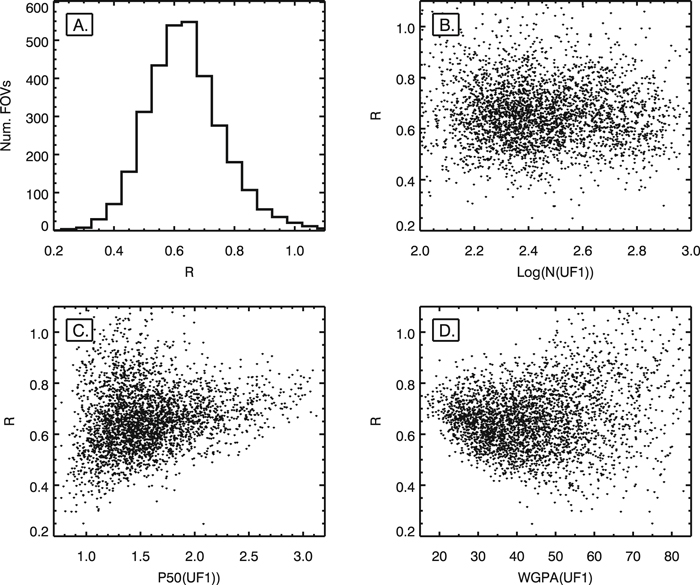
Figure C4. Behaviors of the ratio R (WGPA for UF0 stars divided by WGPA for UF1 stars) for each FOV. (Top left, panel A) Histogram of R values. The mean is 0.66 and the standard deviation is 0.12. (Top right, panel B) R as a function of log N of the number of UF1 stars in each FOV. (Bottom left, panel C) R as a function of the median debiased polarization percentage P50 for UF1 stars in each FOV. (Bottom right, panel D) R as a function of WGPA for the UF1 stars in each FOV. There are very few FOVs with low R and high P50 or with low R and low WGPA.
Download figure:
Standard image High-resolution imageThe similar plots of R versus P50 (Figure C4(C)) and WGPA (Figure C4(D)) show a couple of possible trends. In the R versus P50 plot, Figure C4, panel C, there is an absence of low R values where P50 values are high, which suggests that UF1 and UF0 stars in such fields are equally sampling the magnetic field orientations there. In the R versus WGPA plot, panel D, there is also an absence of low R values where WGPA values are small. The same explanation likely applies, that in regions where the magnetic field is more coherent, and WGPA values are therefore small, UF1 values are not greatly different from UF0 ones.
Where R has the greatest spread include low-P50 and high-WGPA FOVs. In those FOVs, R values can be as small as 0.2, likely because the UF0 GPA histogram has collapsed due to having too few constituent stars per FOV. Some R values for low-P50 and high-WGPA FOVs exceed unity, again likely signifying too few UF0 stars are present with which to form meaningful GPA histograms. While UF0 stars, and UF1 stars, are both fine for sampling FOVs where P50 is high and WGPA is low, UF1 stars appear to be better for sampling the low-P50 and/or high-WGPA FOVs.
The greatest confidence polarization properties will be obtained by selecting the greatest P'S/N values, such as those of the P'S/N ≥ 3 UF0 subset. However, even across the 76 deg2 of the inner Galactic plane surveyed by GPIPS, such stars are relatively rare. The UF0 stars account for only 2.8% of the stars measured for polarization and sample the survey area at 70'' mean separation. Relaxing the P'S/N criterion admits some low-confidence polarization values, but does not appear to introduce strong log N, P50, GPA, or WGPA biases relative to the UF0 subset and may avoid possible problems associated with the UF0 stars in the low-P50 FOVs. The UF1 WGPA values are greater than the UF0 ones, but by a mostly predictable ratio. Also, electing to characterize the Galactic disk magnetic field properties via the UF1 subsample increases the stellar probe numbers by more than a factor of 4, leading to halving of the mean angular sampling separation. For the purposes of the FOV-based median comparisons of polarization (magnetic field orientation) properties offered in the text, the UF1 choice seems appropriate. User-based studies must carefully assess their own selection criteria against their specific science goals.
The overall conclusion is that the UF1 selection criteria result in FOV-based samples of stars with measured polarization properties that are able to probe and characterize magnetic field orientations adequately and without the possible biases (especially against low-P50/high-WGPA FOVs) introduced when adding additional P'S/N cutoffs.
Appendix D: Alternate Displays for Figures 12–15
This section offers representations of Figures 12 through 15 using color look-up tables better suited to individuals with CVD and to enable others to distinguish finer details than presented in those figures in the text.
Production of Figures D1 through D4 was based on concepts described on website of Paul Tol (https://personal.sron.nl/~pault/#fig:scheme_rainbow_discrete). In particular, the 34 discrete RGB triplet values shown in Figure C1 on that website were copied and interpolated to 245 levels to create a rainbow-like color look-up table (CLUT). New versions of Figures 12 through 15 were constructed using this CLUT (with stretches and inversions as needed to agree best with the original figure versions). To evaluate the effectiveness of the new CLUT, side-by-side comparisons of the new figures with the old figures were performed using the Color Oracle (https://colororacle.org/index.html) tool set to Deuteranopia, which modifies displayed colors to simulate that most common CVD. The new CLUT was judged to do better at retaining discrimination of displayed value to color than was done by the original CLUT. The reproductions of Figures 12 through 15 using the new, CVD-friendly CLUT are shown in the following.
Figure D1 displays the 2D (GL, GB) distribution of the base 10 logarithm of the number counts of UF1 stars in each FOV within GPIPS. Figure D2 displays the similar 2D distribution of the mean percentage polarization P50 of the UF1 stars in each FOV. Figure D3 displays the 2D distribution of the mean Galactic position angle GPA50 of the UF1 stars in each FOV. Figure D4 displays the 2D distribution of the interquartile ranges of the GPA distribution of UF1 stars in each FOV.
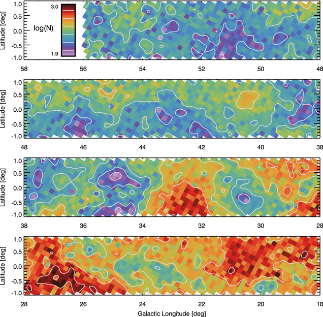
Figure D1. Representation of Figure 12: false-color representation of the base10 log of the number of UF1 stars in each of the GPIPS FOVs, vs. Galactic longitude and latitude, as four longitude slices. Color look-up rectangle, with six nearly equally spaced gray contours, corresponding to 100, 150, 225, 340, 500, and 750 UF1 stars per FOV, is shown in the top slice. The smallest number of UF1 stars in any FOV is 64, the largest is 1112. Note that extinction and the Galactic bulge both likely play roles in the variations in the numbers of detected stars with direction.
Download figure:
Standard image High-resolution image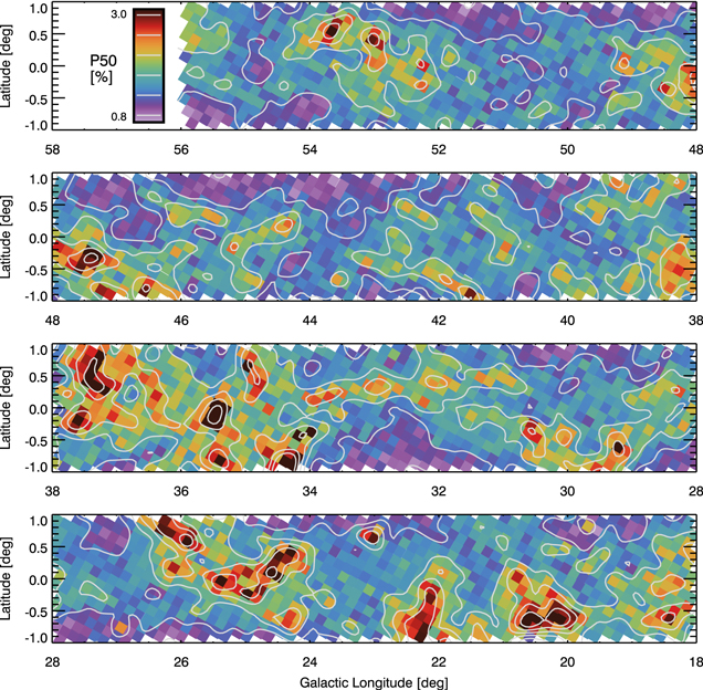
Figure D2. Representation of Figure 13: Galactic longitude and latitude distribution of the median percentage polarization P50 in each GPIPS FOV. Polarization medians range from around 0.8% to over 3% in the H band, with a weak tendency to be higher along the disk midplane. Six gray contour levels corresponding to P50 values of 0.9%, 1.3%, 1.7%, 2.1%, 2.5%, and 2.9% are drawn over the false-color panels and inside the color look-up rectangle in the top panel.
Download figure:
Standard image High-resolution image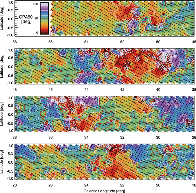
Figure D3. Representation of Figure 14: Galactic longitude and latitude distribution of GPA50 in each GPIPS FOV in the same four-slice presentation as in the previous figures. Unlike in Figure 14, look-up table colors here do not wrap around 0° and 180°, so aliasing is more prominent;y seen. Black lines within each FOV box indicate the GPA orientation. Six gray contour levels, corresponding to GPA50 values of 15°, 45°, 75°, 105°, 135°, and 165°, and one red contour, corresponding to the disk-parallel GPA50 value of 90°, are drawn over the false-color panels and inside the color look-up rectangle in the top panel.
Download figure:
Standard image High-resolution image
Figure D4. Representation of Figure 15: Galactic longitude and latitude distribution of WGPA, the interquartile ranges of the GPA distributions in each of the GPIPS FOVs. The color look-up rectangle in the uppermost panel indicates that WGPA values range from a low of about 15° (red colors) to a high of about 80° (dark blue colors). Six gray contour levels corresponding to WGPA values of 20°, 31°, 42°, 54°, 64°, and 75° are drawn over the false-color panels and inside the color look-up rectangle in the top panel. Note that the value to color mapping in this figure is inverted from previous figures to highlight the low-WGPA regions in darker red colors.
Download figure:
Standard image High-resolution imageFootnotes
- 4
Available in full form from http://sites.bu.edu/gpips and in more limited form from the Infrared Science Archive (IRSA) at https://irsa.ipac.caltech.edu/data/GPIPS/overview.html.
- 5
GPIPS observing modes evolved from seven sky pointings, with 17 HWP images at each pointing direction for 119 total images in the earliest years, to six sky pointings with 17 HWP images (102 total images), and finally to six pointings of 16 images (96 total images per FOV).
- 6
GPIPS debiased linear polarization percentages follow Paper I such that
 for the case where the measured PRAW is greater than its uncertainty σP and zero otherwise.
 - 7
Angle aliasing in the GPA histogram was reduced by accumulating the Gaussian probability distributions across an angle range 11 times wider than the usual 0°–180° range, instead of truncating at the range boundaries, and then shifting and adding the probabilities outside the usual range into the bins within that range.
- 8
Planck Collaboration et al. (2015) reported position angles ψ for the peak of the electric field vector, which is perpendicular to the magnetic field orientation for thermal dust emission. Those angles are rotated by 90° here to become GPA values.