Fundamental Principles for Daylight Calculation Methods

Abstract

Historically, the sky vault in hemispheric form was the geometrical image used to define angular sun coordinates. The same sky hemisphere concept was employed to describe the luminance distribution over the vast endless upper half-space and to visually represent particular solid angles on that sky. Therefore, any object, the sun, building, window aperture, etc., could be projected from an illuminated point or surface element onto the sky hemisphere and thus the spherical area would represent the solid angle and, if the radius of the hemisphere is equal to unity, the solid angle would be in steradians. And so the sky hemisphere could instructively show its overall luminance pattern as well as the luminance of each of its surface elements that pass the scattered skylight in all directions to its center. Thus, in contrast to parallel sunbeam illumination directed from the sun position, the skylight is distributed to ground level from the whole upper half-space. The advantage of this hemispheric sky model is that all surface elements have their normal directed to the sphere center, i.e., have the most efficient position indicating also a defined most effective solid angle.

Appendix 7

7.1.1 Comparison of Basic and Approximate Formulae for Defining the Window Solid Angle

The most extensive light source present everywhere during daytime is the vast sky extending from the horizon to the zenith. The theoretical image of the sky vault is a hemisphere which represents the whole upper half-space that can be measured in solid angle units, i.e., steradians (see in Appendix 2).

Originally, the whole space was simulated by the surface of a sphere with unity radius, ${A_0} = {\omega_{\rm{s}}} = 4\pi$; thus, the sky hemisphere has area $A = 6.283185\,{\hbox{sr}}$.

The basic rule for defining illuminance from the area source on any sloped surface element ${\hbox{d}}{E_{\rm{vi}}}$ is determined by the elemental solid angle of the source plane projected onto the horizontal illuminated plane ω _p multiplied by the source luminance ${L_{\rm{vs}}}$, i.e.,

$$ {\hbox{d}}{E_{\rm{vi}}} = {L_{\rm{vs}}}\,{\hbox{d}}{\omega_{\rm{p}}}({\hbox{lx}}). $$

(A7.1)

As shown in detail in Chaps. 3–5 the typical sky luminance distributions are now standardized in the ISO/CIE general sky, including the simplest Lambertian uniform sky as sky type 5 in relative terms. If ${L_{\rm{vs}}} = 1$, the task is to determine the projected solid angle

$$ {\hbox{d}}{\omega_{\rm{p}}} = {\hbox{d}}{\omega_{\rm{s}}}\,cos\,i\,({\hbox{sr}}). $$

(A7.2)

where ${\hbox{d}}\omega$ is the solid angle element in which the area light source illuminates an element of the plane with any slope and azimuth orientation given by the incidence angle i after (3.24).

The horizontal plane was taken as the most frequent working plane of visual tasks (e.g., for handwork on a bench or reading on a table). Then its normal point to the zenith, $i = Z = 0^\circ$ or $i = \varepsilon = \pi /2 = 90^\circ$, if either the zenith angle $Z$ or the elevation angle $\varepsilon$ is taken into account.

So, the Lambert sky hemisphere or the ISO/CIE sky type 5 with a certain unity uniform luminance ${L_{\rm{vs}}}$ will illuminate the outdoor horizontal plane in the whole sky solid angle and its projection onto the plane coincides with the area of the hemisphere base; thus, ${\omega_{\rm{ph}}} = \pi$ and

$$ {E_{\rm{vi}}} = {D_{\rm{v}}} = 3.1415926\,{L_{\rm{vs}}}({\hbox{lx}}). $$

(A7.3)

Such cases sometimes happen in reality, e.g., during dense foggy situations under an overcast sky when ${L_{\rm{vs}}}/{D_{\rm{v}}} = 1/\pi = 0.31831$.

Owing to the common architectural design and building practice involving vertical and horizontal grids of daylight obstructions and apertures, the classical division of solid angular nets cuts the hemisphere in vertical and horizontal lunes as shown e.g., in Figs. A3.3 and A3.5. Such lunes form spherical double-angle areas determined by the widest angle either on the horizon or on the section meridian of the virtual hemisphere with equal solid angles:

$$ {\hbox{d}}\omega = {\hbox{d}}{\varphi_0}\int\limits_{\varepsilon = 0}^{\pi /2} {\sin \,\varepsilon \,{\hbox{d}}\varepsilon = {\hbox{d}}{\varphi_0}\, \times \,1} \,({\hbox{sr}}) $$

(A7.4)

or

$$ {\hbox{d}}\omega = {\hbox{d}}{\varepsilon_0}\int\limits_{\varphi = 0}^\pi {\sin \,\varphi \;{\hbox{d}}\varphi = {\hbox{d}}{\varepsilon_0} \times 2} ({\hbox{sr}}) $$

(A7.5)

In both equations above and in all further relations 1 sr = rad² because the double-sided lune is ${A_{\rm{p}}} = 2{\varphi_0}$or $2\,{\hbox{d}}{\varepsilon_0}$ (note that if ${\varphi_0}$ is in degrees then ${A_{\rm{p}}} = \pi {\varphi_0}^\circ /90^\circ$).

It is evident that ${\varphi_0}$ lunes coincide with solid angles of endlessly high rectangular openings or vertical obstructions, whereas $2\,{\varepsilon_0}$ lunes are valid for endlessly long obstruction barriers on both sides (walls or house fronts) and illuminating aperture strips such as rows of windows, sawtooth or zenith top lights, and street or atrium openings.

Lambert realized that the old Maurolyco’s pyramid concept is in fact the image of the solid angle of any rectangular light source in an upright position like a window. That was a logical approach to define its illuminance influence on the horizontally placed surface element. But this pyramid has to be imagined for a vertical window in the simplest configuration with its peak point M and one base corner of the pyramid P placed on a normal line from the bottom corner of the window (Fig. A7.1). Thus, such a pyramid does not have the form of a true pyramid, but it is in fact a pyramid with its peak at the side corner of a rectangle. Although Lambert used a coordinate system different from current one, using the coordinate system in Fig. A7.2 with the dimensions $x,y,z$ when the diagonal is ${d_{\rm{r}}} = \sqrt {{x^{2\,}} + {y^2} + {z^2}}$, one can define the dominant (normal) maximal angles of the lune by any trigonometric function of either the azimuth angle ${\varphi_0}$ or the elevation angle ${\varepsilon_0}$, i.e.,

Fig. A7.1

Simplified Lambert scheme of a rectangular light source

Fig. A7.2

Solid window angle and its projection onto the horizontal plane and coordinates

$$ \tan {\varphi_0} = y/x\quad {\hbox{or}}\quad \tan {\varepsilon_0} = z/x, $$

(A7.6)

$$ \cos \,{\varphi_0} = \frac{x}{{\sqrt {{x^2} + {y^2}} }}\quad {\hbox{or}}\quad \cos \,{\varepsilon_0} = \frac{x}{{\sqrt {{x^2} + {z^2}} }}\,,{\hbox{etc}}{.} $$

(A7.7)

Knowing the perspective principle that two parallel lines intersect at infinity at the vanishing point, one can imagine a double system of lune solid angles on the virtual sky hemisphere with unity radius. Specifically:

• One solid angle formed by an endlessly high vertical window with maximum azimuth angle ${\varphi_0}$ which has the half-lune area equal to the solid angle ${\omega_{\rm{s}}} = {\varphi_0}/2$.

• Another horizontal lune for an endlessly wide (on both sides) horizontal aperture projected on the sky hemisphere has area, i.e., solid angle equal to, ${\omega_{\rm{s}}} = {\varepsilon_0}$ _.

Finally, Lambert’s mathematical formula as well as Wiener’s (1884) geometrical relation is valid for a window solid angle projected onto the horizontal plane with the bottom window frame in the illuminated plane:

$$ {\omega_{\rm{ph}}} = \frac{1}{2}\,({\phi_{0\,}} - {\phi_{01\,}}\,\cos \,{\varepsilon_0}). $$

(A7.8)

The vanishing tendency of both lunes from ${\varphi_0}$ or ${\varepsilon_0}$ to zero cannot be represented by the reduction in relation to only the cosine angle as Lambert (1760, paragraph 181) suggested the form expressing $\upsilon = {\varphi_{01}}$ as its tangent value:

$$ \tan \upsilon = \tan {\varphi_{01}} = \tan {\varphi_0}\,cos{\varepsilon_0} = \frac{y}{{\sqrt {{x^2} + {z^2}} }}. $$

(A7.9)

Thus, an approximation ignoring a slight reduction of y due to the ${\varepsilon_0}$ droop line and thus the following classical formula is in the form:

$$ {\omega_{\rm{ph}}} = \frac{1}{2}\,\left( {{ \arctan }\,\frac{y}{x} - \frac{x}{{\sqrt {{x^2} + {z^2}} }}\,{ \arctan }\,\frac{y}{{\sqrt {{x^{2\,}} + {z^2}} }}} \right)\;\;. $$

(A7.10)

Moon and Spencer (1946) derived the same formula using the vector method, but Moon (1936, 1961) presented a similar form

$$ {\omega_{\rm{p}}} = \frac{1}{2}\,\left( {\arctan \,\frac{y}{x} - \frac{x}{{\sqrt {{x^2} + {y^2} + {z^2}} }}\,\arcsin \,\frac{y}{{\sqrt {{x^{2\,}} + {y^2} + {z^2}} }}} \right), $$

(A7.11)

which was probably influenced by Yamauti (1924), whom he regarded as the first to derive it.

Of course, in those days all researchers were investigating the measuring or graphical possibilities to simplify the “direct daylight factor,” i.e., sky factor calculations, and user-friendly graphical tools for its estimation and did not consider any sky luminance distributions obeying Lambert’s assumption ${L_{\rm{vs}}} = 1$. The so-called Lambert formula was derived using the interrelation in (A7.9) and (A7.10) after Fig. A7.1:

$$ {E_{\rm{vi}}}{ = }{L_{\rm{vs}}}\frac{{({\varphi_0} - {\varphi_{01}}\cos {\varepsilon_0})}}{2} = { }{L_{\rm{vs}}}{ }\frac{{\left[ {{\varphi_0} - \cos {\varepsilon_0}\arctan (\cos {\varepsilon_0}\,\tan {\varphi_0})} \right]}}{2}({\hbox{lx}}). $$

(A7.12)

Several researchers followed this formula and considered the interdependence between $\varepsilon$ and $\varphi$ angles defined in (A7.9) in several trials to find some further approximations for a window without a sill in the case of a horizontal or a vertical illuminance after the classical integration or the vector method for the uniform rectangular source (Herman 1900; Higbie 1925) as well as circular sources (Jones 1909, 1910). Walsh (1961), Moon and Spencer (1946) praised “the masterly presentation of the basic methods by Stevenson” (1933b), who summarized the mathematical and graphical estimations of the solid angle measurements and grilles, mentioning also some errors and approximations. In an earlier study, Stevenson (1931) treated in addition to both vertical section planes with divisions of the sky hemisphere in orthogonal projection, also the horizontal plane and stated the basic relation

$$ {E_{\rm{vi}}} = {L_{\rm{vs}}}\int\limits_0^{{\varphi_0}} {\int\limits_0^{{\varepsilon_0}} {\sin \varepsilon \,\cos \varepsilon \,{\hbox{d}}\varepsilon \,{\hbox{d}}\varphi } } \,({\hbox{lx}}). $$

(A7.13)

This integration yielded him the relation

$$ {E_{\rm{vi}}} = \frac{{{L_{{\rm{vs}}\,}}{\varphi_0}}}{2}({\sin^2}\,{\varepsilon_0}) = \frac{{{L_{{\rm{vs}}\,}}{\varphi_0}}}{4}[1 - \cos (2{\varepsilon_0})]\,({\hbox{lx}}) $$

(A7.14)

but left out the interdependence between the lune intersection, i.e., the relation between ${\varepsilon_0}$ and ${\varphi_0}$. So, this was the simplest approximation formula with the desired separation of independent influences of ${\varepsilon_0}$ and ${\varphi_0}$ angles which suited the construction of diagrams by Waldram and Waldram (1923) and Waldram (1980) or the design of protractors by Stevenson (1932, 1933a), Dufton (1940) and Danilyuk (1941). All mentioned some approximations but defined none. However, and without just cause, as will be explained, Moon and Spencer (1946) declared the Waldram method “worthless” for a long rectangular source as it “completely ignores the correct equations which are employed by the rest of the world.” So the question is what is the correct method.

The exact integration has to follow the original equation:

$$ {E_{\rm{vi}}} = {L_{\rm{vs}}}\int\limits_{\varphi = 0}^{{\varphi_0}} {\left[ {\int\limits_0^{{\varepsilon_0}\left( \varphi \right)} {\sin \varepsilon \,\cos \varepsilon \,{\hbox{d}}\varepsilon } } \right]} \;{\hbox{d}}\varphi = \frac{{{L_{\rm{vs}}}}}{4}\int\limits_{\varphi = 0}^{{\varphi_0}} {\left\{ {\,1 - \cos \left[ {2{\varepsilon_0}(\varphi )} \right]\,} \right\}} {\hbox{d}}\varphi \,({\hbox{lx}}) $$

(A7.15)

when

$$ \tan {\varepsilon_0}(\varphi ) = \tan {\varepsilon_0}\,cos\,\varphi. $$

(A7.16)

Thus, the equation to be integrated is

$$ {E_{\rm{vi}}} = \frac{{{L_{\rm{vs}}}}}{4}\int\limits_{\varphi = 0}^{{\varphi_0}} {\left\{ {1 - \cos [2\arctan (\cos \varphi \,\tan {\varepsilon_0})]\,} \right\}} {\hbox{d}}\varphi \,({\hbox{lx}}), $$

(A7.17)

which is analytically unsolvable, but can be relatively precisely solved by numerical integration, i.e., summation of tiny elements ${\hbox{d}}\varphi = ({\varphi_2} - {\varphi_1})/1,000$. The computing time is usually some milliseconds for a typical PC (operating at a frequency above 1 GHz). The numerical error is then below 0.1% for any type of integration method (including the simplest one – the trapezoidal integration method).

A further simplification of (A7.17) can be done by assuming that for very small ${\varepsilon_0}$ and ${\varphi_0}$ angles their tangents are equal to their radian values; thus,

$$ {\hbox{Evi}} = \frac{{{L_{{\rm{vs}}\,}}{\varepsilon_0}^2}}{4}\left[ {{\varphi_0} + \frac{{\sin (2{\varphi_0})}}{2}} \right] = \frac{{{L_{{\rm{vs}}\,}}{\varepsilon_0}^2}}{4}[{\varphi_0} + \sin \,{\varphi_{0\;}}\cos \,{\varphi_{0\;}}]\,({\hbox{lx}}). $$

(A7.18)

The results obtained after use of all three main simplification formulae, i.e., Lambert’s (A7.12), Stevenson’s (A7.14), and exact integration assuming small angles (A7.18), and the exact results after (A7.17) were also published (Kittler et al. 2010), where the derivation was done for a window placed sideways from the coordinate zero point.

The approximation errors can be followed here with a simplified case with regard to the different window width angle ${\varphi_0}$ in the relative illuminance horizontal level for selected window elevation angles ${\varepsilon_0}{ = 2}0^\circ, {5}0^\circ, \;{\hbox{and 75}}^\circ$ in Fig. A7.3. It is evident that the exact calculation after numerical integration after (A7.17) gives results almost identical to those obtained with the traditional Lambert formula (A7.12) in all cases with an error of less than 0.1%.

Fig. A7.3

Comparison of the relative illuminances obtained by approximate formulae and by numerical integration

Although the differences seem to be quite small, some errors might be significant, e.g.:

• If the window is relatively narrow (${\varphi_0}$ under 45°) even if it is quite high (${\varepsilon_0}$ over 50°), e.g., owing to the illuminated point being close to the window, all approximate formulae give good results except for (A7.18) when the window is too high. So in real cases these illuminance errors seem to be practically unimportant unless the sky luminance pattern is far from uniform.

• If the width angle is very wide, e.g., ${\varphi_0} = 50-90^\circ$, the error increases after (A7.14) and the relative percentage error after Fig. A7.4 rises in accordance with the width angle, with the maximum of 100% error if ${\varepsilon_0} = 20^\circ$ and ${\varphi_0} = 50^\circ$, which seems to be an enormous error.

  Fig. A7.4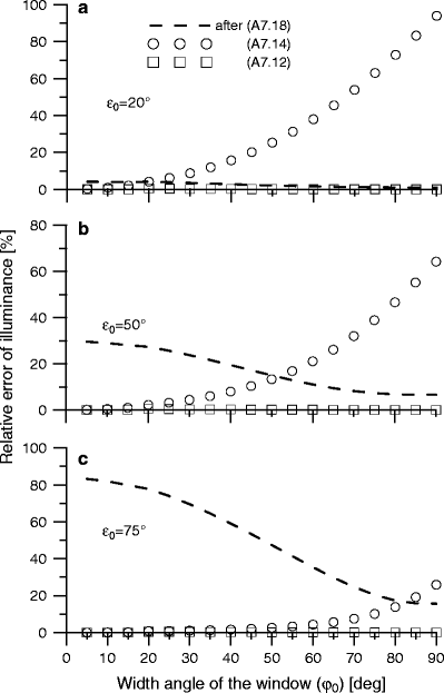

  

  Relative errors connected with approximations

• If the separation of ${\varepsilon_0}$ and ${\varphi_0}$ influences is realized after (A7.18), the exaggerated errors can occur under higher apertures but small width angles as documented in Fig. A7.4c.

Separation of the influences of ${\varepsilon_0}$ and ${\varphi_0}$ angles is possible after (A7.14) with relatively small errors when both these angles are small. With respect to the advantages of the Waldram diagrams – a very clear and illustrative “design and check” oriented tools criticized by Moon and Spencer (1946) cannot be justified because the approximation errors in the case of very wide windows are compensated by the droop-line reductions following the lune vanishing points. A comparison of the results obtained with graphical diagrams or protractors is given in the appendix in Chap. 8. In fact the droop-line tool was used earlier by Molesworth (1902) for graphical estimation of obstructions, while Pleier (1907) measured obstractions by solid angles.

References

Beer, A.: Grundriss des photometrischen Calcüles. Vieweg Verlag, Braunschweig (1854)
Burchard, A.: Die natürliche Beleuchtung der Strasse. Zentralblatt der Bauverwaltung, 7–8, 38–39 (1919a)
Burchard, A.: Die natürliche Beleuchtung des Hofes. Zentralblatt der Bauverwaltung, 100, 597–600 (1919b)
CIE – Commission Internationale de l´Éclairage: Natural Daylight, Official recommendation. Compte Rendu CIE 13th Session, 2, part 3.2, 2–4 (1955)
CIE – Commission Internationale de l´Éclairage: Spatial distribution of daylight – CIE Standard General Sky. CIE Standard S 011/E:2003, CB CIE Vienna (2003)
Cox, H.: The law and science of ancient lights. H. Sweet, Law Publ., London (1871)
Du, J. and Sharples, S.: Daylight in atrium buildings: Geometric shape and vertical sky components. Lighting Res. Technol., 42, 4, 385–397 (2010)
ISO – International Standardisation Organisation: Spatial distribution of daylight – CIE Standard General Sky. ISO Standard 15409:2004 (2004)
Kastendeuch, P.P. and Najjar, G.: Simulation and validation of radiative transfers in urbanised areas. Solar Energy, 83, 3, 333–341 (2009)
Kittler, R., Ondrejička, Š., Tiňo, J.: Základy výpočtových metód osvetlenia z plošných zdrojov. (Basis of illumination calculation methods from planar sources) Private Res. Report, Institute of Construction and Architecture, Slovak Academy of Sciences, Bratislava (1962)
Kittler, R. and Mikler, J.: Zaklady vyuzıvania slnecneho ziarenia. (In Slovak. Basis of the utilization of solar radiation.) Veda Publ., Bratislava (1986)
Kittler, R. and Pulpitlova, J.: Basis of the utilization of daylight. (In Slovak. Zaklady vyuzıvania prırodneho svetla). VEDA Bratislava (1988)
Kittler, R.: Comment 2 on Matusiak, B., Aschehoug, Ø., 2002, Light. Res. and Technol., 34, 2, 145–147 (2002)
Lambert, J.H.: Photometria sive de mensura et gradibus luminis, colorum et umbrae. Augsburg (1760), German translation by Anding, E.: Lamberts Fotometrie. Klett Publ., Leipzig (1892), English translation with introduction notes by DiLaura D.L.: Photometry, or On the measure and gradation of light, colors and shade. Publ. IESNA, N.Y. (2001)
Littlefair, P.: Daylight prediction in atrium buildings. Solar Energy, 73, 2, 105–109 (2002)
Markus, T.A. and Morris, E.N.: Buildings, climate and energy. Pitman Publ. Ltd., London (1980)
Matusiak, B., Aschehoug, Ø., Littlefair, P.: Daylighting strategies for an infinity long atrium: An experimental evaluation. Light. Res. and Technol., 31, 1, 23–34 (1999)
Matusiak, B. and Aschehoug, Ø.: Algorithms for calculation of daylight factors in streets. Light. Res. and Technol., 34, 2, 135–147 (2002)
Pianykh, O.S., Tyler, J.M., Waggenspack, W.N.: Improved Monte Carlo form factor integration. Computer Graphics, 23, 6, 723–734 (1998)
Seshadri, T.N.: Equations of sky component with a CIE standard overcast sky. Proc. Indian Acad. Sci., 57A, 233–242. (1960)
Sharples, S. and Lash, D.: Reflectance distributions and vertical daylight illuminances in atria. Lighting res. Technol., 36, 1, 45–57 (2004)
Swarbrick, J.: Easements of light. Vol. I. Modern methods of computing compensation. Batsford Ltd., London, Wykeham Press, Manchester (1930)
Tregenza, P. and Sharples, S.: Daylight algoritms. Report ETSU, University of Sheffield (1993)
Waldram, P.J. and Waldram, J.M.: Window design and the measurement and predetermination of daylight illumination. Illum. Engineer, 16, 4–5, 90–122 (1923)
Waldram, P.J.: A measuring diagram for daylight illumination. Batsford, London (1950, 1980)
Walsh, J.W.T.: The Science of Daylight. Macdonald Publ., London (1961)
Zahn, J.: Oculus Artificialis Telediptricus sive Telescopium. Würzburg (1686, 1702)
References to Appendix
Danilyuk, A.M.: Raschot yestestvennogo osveshcheniya pomeshcheniy. (In Rusian. Calculation of natural illumination of rooms.) Gos. Izdat. Stroyit. Liter., Moscow, Leningrad (1941)
Dufton, A.F.: The computation of Daylight Factors in factory design. Journ. Sci. Instr., 17, 9, 226–227 (1940)
Herman, R.A.: A treatise on geometrical optics. Cambridge University Press, Cambridge (1900)
Higbie, H.H.: Prediction of daylight from vertical windows. Transac. IES, N.Y. 20, 5, 433–437 (1925)
Jones, B.: The mathematical theory of finite surface light sources. Transac. I.E.S., 4, 216–239 (1909)
Jones, B.: On finite surface light sources, Transac. I.E.S., 5, 281–299 (1910)
Kittler, R., Kocifaj, M., Darula, S.: The 250th anniversary of daylight science: Looking back and looking forward. Light. Res. and Technol., 42, 4, 479–486 (2010)
Lambert, J.H.: Photometria sive de mensura et gradibus luminis, colorum et umbrae. Klett Publ., Augsburg (1760), German translation by Anding, E.: Lamberts Fotometrie. Klett Publ., Leipzig (1892), English translation by DiLaura, D.L.: Photometry, or On the measure and gradation of light, colors and shade. Publ. IESNA, N.Y. (2001)
Molesworth, H.B.: Obstruction to light. Spon and Co., London (1902)
Moon, P.: Scientific basis of illuminating engineering. Dover Publ. Inc., New York (1936, 1961)
Moon, P., Spencer, D.E.: Light distribution from rectangular sources. Journ. Fraklin Inst., 241, 3, 195–227 (1946)
Pleier, F.: Measurement of the stereo-angle of skylight. Proc. Congrés Internat. D´Hygiene Scolaire. I, 362 (1907)
Stevenson, A.C.: On the mathematical and graphical determination of direct Daylight Factors. Proc. Intern. Illumination Congress. Reprinted in an extract by Swarbrick, J. (1933), in Appendix I., p.146-160 (1931)
Stevenson, A.C.: The photographic and visual determination of direct Daylight Factors. Journ.Sci. Instruments, 9, 3, 96. Reprinted by Swarbrick, J. (1933), in Appendix II., p.168-180 (1932)
Stevenson, A.C.: The construction of Daylight Factor grilles. In: Swarbrick, J. (1933), Chapter VI, 99–121 (1933a)
Stevenson, A.C.: On direct Daylight Factor and its estimation. In: Swarbrick (1933), Chapter VII, 122–145 (1933b)
Waldram, P.J.: A measuring diagram for daylight illumination. Batsford, London (1980)
Wiener, C.: Lehrbuch der darstellenden Geometrie, Vol. I. B.G. Taubner Verlag, Leipzig (1884)
Yamauti, Z.: Geometrical calculation of illumination. Researches of the Electrot. Lab., Tokyo, 148 (1924)
Author information
Authors and Affiliations
Corresponding author