10. Predictability

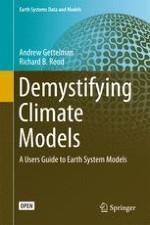
Uncertainty depends in part on the underlying physics of the problem. Some problems are better constrained than others, and this affects our ability to predict them. In climate simulation, the global average temperature is often used as a metric. This implies an average over time and over space. The global average temperature is a fairly well-constrained number: Global averages of the incoming and outgoing energy at the top of the atmosphere and assumptions about the ocean heat uptake allow a pretty good estimate of the global average temperature. This is because the physics of energy conservation are fairly straightforward. Energy comes in from the sun. Some is reflected and some is absorbed by the surface, and then some is radiated back. There are complex constraints on how much energy is absorbed, is reflected, or remains at the surface, mostly related to cloud processes and the ocean circulation, as illustrated in the energy budget diagram (Fig. 10.1).³ But the global energy flows have limits, and the physics (conservation of energy) are fairly certain. Some of them offset each other as well. Nonetheless, we cannot predict the year-to-year variations very far in advance (more on this later).

There are other aspects of climate and efforts at prediction that are not as certain and do not have strong constraints. Prediction of regional distributions of rainfall, for example, is not as well constrained by total energy budgets. In addition to local evaporation and precipitation, air motions bring moisture sources into a region from various and changing direction. The total available energy in a region for precipitation depends on the global atmospheric circulation. It may also depend on details of cloud processes. So predicting the distribution of rainfall at any location is much less certain than global quantities due to the basic physical constraints.

Another aspect of uncertainty related to the underlying physics is the level of variability. Recall Fig. 9.​2, with two distributions having the same mean but different variance (represented by the standard deviation). If the variance is high, we may not be very good at prediction, since the quantity is highly uncertain. Global average temperature is an example of a distribution with low variance, whereas regional rainfall is a distribution with high variance. Higher variances are harder to limit and predict, often because our knowledge of the distributions is low. It is hard to tell if a signal (change in mean, for example, or change in variance) is significant if there is a large amount of variability. The local temperature example in the introduction to this chapter is an example of this. A temperature deviation from a mean by 4 °F (2 °C) is hard to detect if the variance is large, usually measured as a standard deviation from the mean (see Chap. 9). The probability of the deviation’s being “significant” depends on how variable the distribution is, so larger variability (standard deviation) yields less certainty.

The concept of variability is used to help understand the difference between a “signal”, and “noise.”⁴ The signal is a change in the mean: a trend in the climate over time. The noise is the variability that occurs around the mean, such as the variability of a given climate metric from year to year. The larger the variability (noise), the harder it is to see the signal. Higher variability typically occurs on smaller space and time scales. The annual average temperature of a particular location is much more constant than the daily temperature, and the global average temperature varies far less (daily or annually) than does the average temperature in any particular location or region.

Finally, and related to the concept of distributions, impacts often depend on the sensitivity to changes of a distribution. Sensitivity has two aspects. First, we may be worried about extreme events, which are low-probability events at the tail of the distribution. Changes to extreme events are hard to predict because they are low-frequency events, and they have high variability. This is another aspect to uncertainty in prediction that stems from the nature of the physics of climate.

Second, we may worry about events that have thresholds. For example, if the temperature is 68 °F (20 °C), and there is a 1–2°(F or C, F is bigger) uncertainty, that might not matter much. But if the temperature is 32 °F (0 °C), being wrong by a few degrees in either direction makes a big difference: If ice and snow are present and remain, then the weather situation is a whole lot different than if a cold rain falls.

Short-term climate prediction commonly means predicting the climate from the next season to the next decade or two. In many respects, it is similar to weather forecasting. In the climate context, a decade is “short term.” In some sense, the short term is characterized by the period over which the initial state of the system matters: The weather tomorrow depends on the weather today. Other examples include routine seasonal forecasts of expected high and low rainfall one season in advance. Broadly, we are defining “short term” as the period over which the current state of the system matters, and when we can predict the state of some of the internal variability of the climate system.

As described earlier, prediction depends on the problem. Some parts of the system are more predictable than others. In some regions, rainfall in the next season depends on things that are predictable several months in advance, like ocean temperatures. For example, current and predicted temperatures of the tropical Pacific Ocean provide predictive skill for rainfall in western North America.⁶ In other places, like Northern Europe, extremes of precipitation or temperature (both high and low) are usually functions of blocking events, which are weather patterns that persist but are predictable only a week or so in advance. The extent (persistence) of blocking patterns is difficult to predict at all.

Estimates of the near term (whether a week or a season in advance) made with skill can be valuable in preparation. For example, El Niño commonly brings wetter conditions to Southern California, and when a strong El Niño is developing, precautions are often taken to deal with mudslides, especially in regions recently affected by fire. Forecasts of impending tropical cyclone impacts 24–72 hours in advance enable evacuations and staging of rescue and disaster relief.

But high variability that makes predictions uncertain means that they are less useful. As a counterexample, El Niño also alters the frequency of occurrence of tropical cyclones in the Atlantic (hurricanes), because the upper-level winds in the Atlantic blow the opposite way from usual (and in the opposite direction to surface winds). However, while storms are less frequent, even a single storm in an El Niño year can be damaging. In 1992 after a large El Niño, there were only four hurricanes that year in the Atlantic and one major storm (average is six hurricanes and three major ones), but that single storm was Hurricane Andrew, the second most devastating (in financial terms) storm in recent U.S. history. Because the variability of tropical cyclones is extremely large, and the small-probability events are devastating, the improvement in understanding and forecasting may not be that valuable for prediction.

Near-term prediction is very much focused on the current state of the system: What El Niño will do in 6 months depends strongly on the state of the system now. It is very similar to trying to predict the weather a few hours or day ahead. Most of the uncertainty is in the initial state of the system, called initial condition uncertainty. As an example, the El Niño forecast depends strongly on the current state of the atmosphere and ocean; it does not depend on the CO₂ concentration in the atmosphere in 6 months.

Initial condition uncertainty is a common problem between weather and climate prediction: The climate system is usually sampled sparsely with uncertain observations, and we do not know key things to help us “constrain” the system to forecast the weather more than a few days in advance. If we had more and better information (observations of temperature and wind) in the right places, we would be able to reduce initial condition uncertainty.

For climate prediction (e.g., What will the distribution of weather states be next year, in the year 2020, in 2080, or 2200?), initial condition uncertainty dominates over other uncertainty out to decadal scales. This is because there are long-term patterns in the climate system, mostly from the transfer of heat to and from the deep ocean. At scales beyond a few months, it is the evolution of the ocean that governs how the system responds. Figure 10.2 illustrates that initial condition uncertainty is very large and dominates the uncertainty initially but averages out over long periods of time. The weather tomorrow is dependent on today, and El Niño next year is dependent on this year. But the weather and El Niño’s state in 2080 is not dependent on today.

As the example of the weather or El Niño suggests, there are certain scales for which we know the state of how the system is “forced”: Tomorrow’s weather does not depend much on the greenhouse gas concentration. Over the course of a few years, the earth’s energy budget does depend on the greenhouse gas concentration. But this concentration is fairly well known. As we described in Part II, there are sources and sinks of carbon, and these balance to leave a reservoir of carbon in the atmosphere (see Fig. 7.​6). The CO₂ concentration (and that of methane) changes slowly, with variable growth rates, but in the near term—next year, or in the next 10 years—we have a pretty good idea of what will happen. The total use of fossil fuels also changes slowly over time. How much energy did you use in your house this year? How much gas did you use either in your own car, or as part of sharing a ride or using public transportation? Absent major life changes (new house, new job, new car), you can probably project that your use next year will be similar. So it goes for societies in general. Figure 10.3 illustrates the global emissions of carbon. It is a line that trends up a little bit from year to year. You can make a good estimate of next year’s emissions from this year’s, and projecting forward with a line is not too hard.

But over longer periods of time, things change. What will your personal energy use be in 10 years? That depends on where you live, your job, your house, if you have a family. It also depends on how you will use energy. For example, next year you might put some more efficient lights in your house. But in 10 years you might have an electric car, or you might telecommute, or you might have solar panels, and it might be the same house or a different house. So the uncertainties on your energy use increase. And the uncertainties on your carbon emissions get larger. For instance, you will probably still have a refrigerator. We can probably guess it will use a similar amount of energy as today (maybe you will have the same refrigerator), but maybe you (or your utility) will get the energy for that appliance from solar or wind or gas rather than coal. Those changes mean more variability in the future. Figure 10.4 shows the same data as Fig. 10.3, but now from 1850 to 2011. Now the use is harder to project into the future. If the plot stopped in 1900 or 1950, the “projection” might be very different from what you would assume today. The mix of fuels would be different: a projection of petroleum use in 1970 would be very different from one made today. And you can guess in the future that it might also be very different, for any number of reasons.

Figure 10.5 shows an example of a plot that does not continue to increase. Figure 10.5 is of another greenhouse gas emission: CCl₂F₂, dichlorodifluoromethane, also called CFC-12,⁷ a refrigerant used in home and industrial coolers from refrigerators in homes to air-conditioning units in cars or buildings. It also happens to contain chlorine (Cl), and when it decomposes in the upper atmosphere this chlorine destroys stratospheric ozone, resulting in the Antarctic ozone hole. As a result of this effect, CFC-12 use has effectively has been banned. Again, projecting the emissions of this substance in 1960 or 1980 into the future would be very different from what actually happened. In the case of CFC-12, it was regulated under the 1986 Montreal Protocol, and eventually production had stopped over most of the planet.

You can see where this is going. Over short periods of time, the basic inputs to a climate model—concentrations of greenhouse gases—are fairly predictable. But over longer periods of time, due to external factors (political oil shocks, new technologies) or regulation (limits or bans on productions or emissions), the inputs can change dramatically. For the historical period, whether for carbon or CFCs, we have a pretty good handle on emissions. However, what does this mean for the future? Will oil use rise, as in Fig. 10.4? Will the Chinese have as many cars per person as in the United States? Or is oil use going to look more like the curve in Fig. 10.5, because either everyone is going to have solar panels on their roofs or we run out of economical supplies of oil.

These are not questions for climate models to answer. They are beginning to be questions for integrated assessment models (see Chap. 8). But the answers (how much oil will be used, and how much CO₂ be will emitted by humans in the year 2080) are highly uncertain. They depend on myriad socioeconomic choices. They are not so much predictions as projections and they represent scenarios. Oil use in the future is dependent on a lot of interrelated things: population, population density, available economical supplies of oil, new technologies, and how all these factors interact. One of the problems of scenarios is predicting the application and spread of disruptive technologies. Integrated assessment models are better at predicting the improving efficiency of refrigerators, or power plants, or solar panels. They are less able to predict the impact of smart phones or creative financing for solar panels.

It should be clear that scenario uncertainty (the red line in Fig. 10.2) grows over time and the inputs to a climate model (emissions of gases that affect climate) become highly uncertain. This occurs for timescales longer than a human generation (20–30 years), which also corresponds to the depreciation lifetime of many fixed investments (like a power plant). The major drivers of these uncertainties are slow-accumulating things, like global population, or commonly used energy systems. They are usually subject to the results of different societal decisions: population growth in China, gas extraction technologies in the United States, economic growth in developing countries (Brazil, India, China), and disruptive technologies (internet, global manufacturing, and so on).

One way to look at this is to look at past projections of the present. Figure 10.6 is a reprint from a 2014 energy policy report from the Office of the President of the United States. The report is political, but the data presented in the figure are simply the consumption of gasoline for vehicles in the United States. In 2006, it was projected that in 2013 the United States would use 10 million barrels (550 million gallons, or about 2 billion liters) of gasoline per day. The projection for 2030 was 12 million barrels per day. But the actual value for 2013 was closer to 8 million barrels per day, and the 2030 forecast estimated in 2014 is only 6 million barrels per day. These are big numbers, with big implications. If we wanted to be 40 % below 2006 consumption in 2030, that would take extreme measures for the 2006 forecast, but that would be the expected scenario in 2014 (without doing anything). So scenarios are forecasts as well, and they are often wrong.

Projections of economic and social indicators span a range of predictability. It is probably pretty easy to estimate population now and for the next few years. But economic growth or prices of commodities? Or use of gasoline? Economic growth estimates are rarely even known until well after the fact (the U.S. government revises all growth figures a few months after they are issued). These errors all compound to become part of the uncertainty in the input scenarios used to drive climate models.

So how do we deal with these scenario uncertainties in climate projections? These are the uncertainties in the forcing of climate. In the absence of making a prediction about what society might do, generally social scientists and economists estimate what is possible, and a range of possibilities (scenarios) are derived. The inputs to climate models are typically outputs of integrated assessment models, driven more by a story translated into quantitative inputs. These scenarios have evolved in complexity over time, but the values and spread have not changed that much. But they are not forecasts, because they depend on human policy decisions and choices (like the CFC-12 curve in Fig. 10.5).

Most climate models now use commonly developed scenarios.⁸ Figure 10.7 illustrates the latest set of scenarios (Representative Concentration Pathways, or RCPs) used to force most climate models.⁹ Figure 10.7 illustrates the scenarios in terms of the radiative forcing of climate in watts per square meter (Wm⁻²) of the earth’s surface. Recall that a watt is the same as the watt in lightbulbs: 60 Wm⁻² is the energy of a typical incandescent bulb, and the solar input is about 160 Wm⁻².¹⁰

Each RCP scenario was designed to reach a specific radiative forcing target from greenhouse gases by a particular date, based on different predictions of what society might do. The levels of CO₂ and other greenhouse gases in the atmosphere that create the forcing are derived for each RCP (Fig. 10.8). CO₂ concentrations are in parts per million (ppm). One part per million means one molecule of CO₂ for every million molecules of air. The current concentration of CO₂ is about 400 ppm, and the level in 1850 before most industry developed was 280 ppm CO₂. That is a 40 % increase. Note that these scenarios are possible futures, just like the different forecasts in Fig. 10.6. We have been on the black curve (high emissions), but Fig. 10.6, and others like it, suggest that we might be transitioning to one of the more moderate curves.

Using common scenarios implicitly says that the scenarios are a major driver of uncertainty, and we need to compare models with common scenarios. Otherwise, the uncertainty due to the scenarios would be hard to assess.

As we shall see, a central theme of future climate prediction is to realize that most of the uncertainty lies not in the models themselves, but in the scenario for emissions (i.e., in the scenario uncertainty). The climate of the future is dominated by scenario uncertainty (the red line in Fig. 10.2), and that uncertainty is from human systems. In the end, climate is our choice, even if it is simply to make no choice about our emissions and continue present policies.

Thus far we have discussed sources of error in climate projections for the far future (beyond several decades) and in the near term (within a decade or two). Throughout this entire period there is a constant source of uncertainty, and this is what we typically think of as the uncertainty in a climate model: the model uncertainty, or the structural uncertainty in how we represent climate (the blue line in Fig. 10.2).

Model uncertainty is our inability to represent perfectly the coupled climate system. It is present in representing each of the components, and each of the processes within the system. The uncertainty has many different forms, and different values. Some uncertainties are large and some are small, mostly related to the physics of the processes. We have discussed a lot of these physical and process uncertainties in detail. Many uncertainties stem from the scales that models must resolve: Small-scale processes that are highly variable below the grid scale of a model are difficult to resolve or approximate. In the atmosphere, clear skies are easier to understand and represent than cloudy skies. In the land surface, variations in soil moisture and vegetation at the small scale interact with moisture and energy fluxes to make things complex.

Complexity arises due to nonlinear effects. In a nonlinear process, the average of results is not the same as if the inputs are averaged. As a simple example, let’s say that the rate of evaporation (R) is the square of the soil moisture (R = S²), where the moisture (S) varies from 0 → 10. If there are two equal-sized areas of a grid box, one with soil moisture of S = 0 and one of S = 10, then the average soil moisture S = 5. But calculating the evaporation from the average yields R = 5² = 25, whereas calculating the rate from each part and averaging (0 and 10² = 100, divided by 2) yields 50: double the rate.

Thus there are many sources of model uncertainty. In the present context of trying to understand the sources of uncertainty, note that model uncertainty is constant over time: It does not increase. Because in the future there are better large-scale constraints than small-scale constraints, uncertainty in the future might even decrease.

Model uncertainty can be broken into parametric and structural uncertainty.¹¹ Parametric uncertainties are those that arise because many processes important for weather and climate modeling cannot be completely represented at the grid scales of the models. Therefore, these processes are parameterized, and there are uncertainties in these representations. An iconic parameterized process is that associated with convective clouds that are responsible for thunderstorms. Thunderstorms occur on much smaller spatial scales than can be resolved by global climate models. Therefore, the net effect of thunderstorms on the smallest spatial scales that the climate model can represent is related to a set of parameters based on physical principles and statistical relationships. Recall that the spatial scale that is resolved by a climate model is several times larger than the spatial size of a single grid point. The conflation of errors of different spatial scales, dependent on parameterizations, is difficult to quantify and disentangle.

Structural uncertainties are those based on decisions of the model builder about how to couple model parameterizations together and how they interact. One class of these errors is the always-present numerical errors of diffusion and dispersion in numerical transport schemes; that is, the errors of discrete mathematics. But a more important structural uncertainty perhaps is how the different parameterizations are put together. For example, let’s say an atmosphere model has convection, cloud microphysics, surface flux, and radiation parameterizations. Typically there is a choice in how to couple parameterizations. Either all the parameterizations are calculated in parallel from the same initial state, called process splitting. Or each one could be calculated one after the other in sequence, called time splitting. Typically in a model with time splitting, the most “important” processes are estimated last. For weather models, this is usually cloud microphysics to get precipitation correct. For climate models, this is usually radiation. In either case, the last process is the most consistent with the sequential state. Either method, however, may create a structural uncertainty: If clouds and radiation are calculated separately in a process split model, then the radiation may not reflect the clouds, and the temperature change from heating or cooling may not add up correctly. These are structural uncertainties from coupling processes. The same uncertainties come from coupling the physical processes to the dynamics in the atmosphere or ocean, and from coupling different components.

The result is an uncertainty graph that looks like Fig. 10.2. Internal variability, which is defined from the initial conditions (green line), is the largest contribution to short-term variability (the next tropical cyclone or blocking event or ENSO does not care much about the level of greenhouse gases), with a significant component of model variability (blue line). Over time (a few cycles of the different modes of variability), this fades, and the uncertainty is dominated by structural uncertainty in the model (blue line). But over long time periods, where the input forcings are themselves uncertain, the scenario variability (red) dominates. The latter break point is approximately where the level of uncertainty in the forcing (i.e., uncertainties in emissions translated into concentrations of greenhouse gases, translated into radiative forcing in Wm⁻²) is larger than the uncertainty in the processes (expressed in radiative terms, Wm⁻²). For climate models, the largest uncertainty is in cloud feedbacks. The uncertainty in cloud feedbacks is about 0.5 Wm⁻² per degree of surface temperature change. So far the planet has warmed about 1–2 °C so the uncertainty due to cloud forcing is about 1 Wm⁻². This uncertainty would indicate that scenario uncertainty will dominate model uncertainty when the uncertainty in future radiative forcing between scenarios reached about 1 Wm⁻². In Fig. 10.7, this would be about 2040–2050 and beyond. The practical significance of this situation will be demonstrated when climate model results are discussed in Chap. 11. But first a few words about using models together in ensembles.