Multi-parametric solution-path algorithm for instance-weighted support vector machines

Abstract

An instance-weighted variant of the support vector machine (SVM) has attracted considerable attention recently since they are useful in various machine learning tasks such as non-stationary data analysis, heteroscedastic data modeling, transfer learning, learning to rank, and transduction. An important challenge in these scenarios is to overcome the computational bottleneck—instance weights often change dynamically or adaptively, and thus the weighted SVM solutions must be repeatedly computed. In this paper, we develop an algorithm that can efficiently and exactly update the weighted SVM solutions for arbitrary change of instance weights. Technically, this contribution can be regarded as an extension of the conventional solution-path algorithm for a single regularization parameter to multiple instance-weight parameters. However, this extension gives rise to a significant problem that breakpoints (at which the solution path turns) have to be identified in high-dimensional space. To facilitate this, we introduce a parametric representation of instance weights. We also provide a geometric interpretation in weight space using a notion of critical region: a polyhedron in which the current affine solution remains to be optimal. Then we find breakpoints at intersections of the solution path and boundaries of polyhedrons. Through extensive experiments on various practical applications, we demonstrate the usefulness of the proposed algorithm.

1 Introduction

The most fundamental principle of machine learning would be the empirical risk minimization, i.e., the sum of empirical losses over training instances is minimized:

where L _i denotes the empirical loss for the i-th training instance. This empirical risk minimization approach was proved to produce consistent estimators (Vapnik 1995). On the other hand, one may also consider an instance-weighted variant of empirical risk minimization:

where C _i denotes the weight for the i-th training instance. This weighted variant plays an important role in various machine learning tasks:

• Non-stationary data analysis: When training instances are provided in a sequential manner under changing environment, smaller weights are often assigned to older instances for imposing some ‘forgetting’ effect (Murata et al. 2002; Cao and Tay 2003).

• Heteroscedastic data modeling: A supervised learning setup where the noise level in output values depends on input points is said to be heteroscedastic. In heteroscedastic data modeling, larger weights are often assigned to instances with smaller noise variance (Kersting et al. 2007). The traditional Gauss-Markov theorem (Albert 1972) forms the basis of this idea.

• Covariate shift adaptation, transfer learning, and multi-task learning: A supervised learning situation where training and test inputs follow different distributions is called covariate shift. Under covariate shift, using the importance (the ratio of the test and training input densities) as instance weights assures the consistency of estimators (Shimodaira 2000). Similar importance-weighting ideas can be applied also to transfer learning (where data in one domain is transferred to another domain) (Jiang and Zhai 2007) and multi-task learning (where multiple learning problems are solved simultaneously by sharing training instances) (Bickel et al. 2008).

• Learning to rank and ordinal regression: The goal of ranking (a.k.a. ordinal regression) is to give an ordered list of items based on their relevance (Herbrich et al. 2000; Liu 2009). In practical ranking tasks such as information retrieval, users are often not interested in the entire ranking list, but only in the top few items. In order to improve the prediction accuracy in the top of the list, larger weights are often assigned to higher-ranked items (Xu et al. 2006).

• Transduction and semi-supervised learning: Transduction is a supervised learning setup where the goal is not to learn the entire input-output mapping, but only to estimate the output values for pre-specified unlabeled input points (Vapnik 1995). A popular approach to transduction is to label the unlabeled samples using the current estimator, and then modify the estimator using the ‘self-labeled’ samples (Joachims 1999; Raina et al. 2007). In this procedure, smaller weights are usually assigned to the self-labeled samples than the originally-labeled samples due to their high uncertainty.

A common challenge in the research of instance-weighted learning has been to overcome the computational issue. In many of these tasks, instance weights often change dynamically or adaptively, and thus the instance-weighted solutions must be repeatedly computed. For example, in on-line learning, every time when a new instance is observed, all the instance weights must be updated in such a way that newer instances have larger weights and older instances have smaller weights. Model selection in instance-weighted learning also poses a considerable computational burden. In many of the above scenarios, we only have qualitative knowledge about instance weights. For example, in the aforementioned ranking problem, we only know that higher-ranked items should have larger weights than lower-ranked items, but it is often difficult to know how large or small these weights should be. The problem of selecting the optimal weighting patterns is an instance of model selection, and many instance-weighted solutions with various weighting patterns must be computed in the model selection phase. The goal of this paper is to alleviate the computational bottleneck of instance-weighted learning.

In this paper, we focus on the support vector machine (SVM) (Boser et al. 1992; Cortes and Vapnik 1995), which is a popular classification algorithm that minimizes a regularized empirical risk:

where R is a regularization term and C≥0 controls the trade-off between the regularization effect and the empirical risk minimization. We consider an instance-weighted variant of SVM, which we refer to as the weighted SVM (WSVM) (Lin et al. 2002; Lin and Wang 2002; Yang et al. 2007):

For ordinary SVM, the solution-path algorithm was proposed (Hastie et al. 2004), which computes the entire SVM solutions for all C exactly by utilizing the piecewise-linear structure of the solutions w.r.t. C. This technique is known as parametric programming in the optimization community (Best 1982; Ritter 1984; Allgower and Georg 1993; Bennett and Bredensteiner 1997), and has been applied to various machine learning tasks including support vector regression (Gunter and Zhu 2007; Wang et al. 2008), the one-class support vector machine (Lee and Scott 2007), the ranking support vector machine (Arreola et al. 2008), and other algorithms (e.g., Fine and Scheinberg 2002; Zhu et al. 2004; Efron et al. 2004; Bach et al. 2006; Rosset and Zhu 2007; Sjostrand et al. 2007; Takeuchi et al. 2009; Kanamori et al. 2009); the incremental-decremental SVM algorithm, which follows the piecewise-linear solution path when some training instances are added or removed from the training set, is also based on the same parametric programming technique (Cauwenberghs and Poggio 2001; Laskov et al. 2006; Karasuyama and Takeuchi 2009). These studies have empirically demonstrated that the solution-path approach is computationally more efficient than other iterative SVM solvers.

The solution-path algorithms described above have been developed for problems with a single hyper-parameter. Recently, attention has been paid to studying solution-path tracking in two-dimensional hyper-parameter spaces. For example, Wang et al. (2008) developed a path-following algorithm for regularization parameter C and an insensitive-zone thickness ε in support vector regression (Vapnik et al. 1996; Mattera and Haykin 1999; Müller et al. 1999). Rosset (2009) studied a path-following algorithm for regularization parameter λ and quantile parameter τ in kernel quantile regression (Takeuchi et al. 2006). However, these works are highly specialized to specific problem structure of bivariate path-following, and it is not straightforward to extend them to more than two hyper-parameters. Thus, the existing approaches may not be applicable to path-following of WSVM because it contains n-dimensional instance-weight parameters c=[C ₁,…,C _n ]^⊤, where n is the number of training instances.

In order to go beyond the limitation of the existing approaches, we derive a general solution-path algorithm for efficiently computing the solution path of multiple instance-weight parameters c in WSVM. This extension involves a significant problem that breakpoints (at which the solution path turns) have to be identified in a high-dimensional space. To facilitate this, we introduce a parametric representation of linear changes in instance weights in the high-dimensional space of the instance-weight parameters c. Using this parametrization, we can construct an algorithm that follows the change of optimal solutions along with the linear change of instance-weight parameters (Fig. 2 schematically illustrates the behavior of our algorithm) in a similar way to the one-dimensional regularization path algorithm. Despite its simplicity and usefulness, it has not been exploited so far in machine learning literature, to the best of our knowledge. We will illustrate that our approach covers various important machine learning problems and greatly widens the applicability of the path-following approach. We also provide a geometric interpretation of a weight space using the notion of critical regions based on the studies of multi-parametric programming (Gal and Nedoma 1972; Pistikopoulos et al. 2007). A critical region is a polyhedron in which the current affine solution remains to be optimal (see Fig. 2). This enables us to find breakpoints at intersections of the solution path and the boundaries of polyhedrons.

The rest of this paper is structured as follows. Section 2 reviews the definition of WSVM and its optimality conditions. Then we derive the path-following algorithm for WSVM in Sect. 3. Section 4 is devoted to experimentally illustrating advantages of our algorithm on a toy problem, on-line time-series analysis, and covariate shift adaptation. Extensions to regression, ranking, and transduction scenarios and their experimental evaluation are discussed in Sect. 5. Finally, we conclude in Sect. 6.

2 Problem formulation

In this section, we review the definition of the weighted support vector machine (WSVM) and its optimality conditions. For the moment, we focus on binary classification scenarios. Later in Sect. 5, we extend our discussion to more general scenarios such as regression, ranking, and transduction.

2.1 WSVM

Let us consider a binary classification problem. We denote n training instances by $\{ (\boldsymbol {x}_{i}, y_{i}) \}_{i=1}^{n}$, where $\boldsymbol {x}_{i} \in { \mathcal{X}}\subseteq\mathbb{R}^{p}$ is an input and y _i ∈{−1,+1} is an output label.

SVM (Boser et al. 1992; Cortes and Vapnik 1995) is a learning algorithm of a linear decision boundary

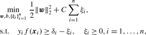
in a feature space ${\mathcal{F}}$, where $\varPhi : {\mathcal{X}} \rightarrow{ \mathcal{F}}$ is a map from the input space ${ \mathcal{X}}$ to the feature space ${ \mathcal{F}}$, $\boldsymbol {w}\in{ \mathcal{F}}$ is a coefficient vector, b∈ℝ is a bias term, and ^⊤ denotes the transpose. The parameters w and b are learned as

(1)

where $\frac{1}{2} \| \boldsymbol {w}\|_{2}^{2}$ is the regularization term, ∥⋅∥ denotes the Euclidean norm, C is the trade-off parameter, and

[1−y _i f(x _i )]₊ is the so-called hinge-loss for the i-th training instance.

WSVM is an extension of the ordinary SVM so that each training instance possesses its own weight (Lin et al. 2002; Lin and Wang 2002; Yang et al. 2007):

(2)

where C _i is the weight for the i-th training instance. WSVM includes the ordinary SVM as a special case when C _i =C for i=1,…,n. The primal optimization problem (2) is expressed as the following quadratic program:

(3)

The goal of this paper is to derive an algorithm that can efficiently compute the sequence of WSVM solutions for arbitrary weighting patterns of c=[C ₁,…,C _n ]^⊤.

2.2 Optimization in WSVM

Here we review basic optimization issues of WSVM used in the following section.

Introducing Lagrange multipliers α _i ≥0 and ρ _i ≥0, we can write the Lagrangian of (3) as

(4)

Setting the derivatives of the above Lagrangian w.r.t. the primal variables w, b, and ξ _i to zero, we obtain

where 0 denotes the vector with all zeros. Substituting these equations into (4), we arrive at the following dual problem:

(5)

where

and K(x _i ,x _j )=Φ(x _i )^T Φ(x _j ) is a reproducing kernel (Aronszajn 1950). The discriminant function $f:{\mathcal{X}} \rightarrow{\mathbb{R}}$ is represented in the following form:

The optimality conditions of the dual problem (5), called the Karush-Kuhn-Tucker (KKT) conditions (Boyd and Vandenberghe 2004), are summarized as follows:

(6a)

(6b)

(6c)

(6d)

We define the following three index sets for later use:

(7a)

(7b)

(7c)

where $\mathcal{O}$, $\mathcal{M}$, and $\mathcal{I}$ stand for ‘Outside the margin’ (y _i f(x _i )≥1), ‘on the Margin’ (y _i f(x _i )=1), and ‘Inside the margin’ (y _i f(x _i )≤1), respectively (see Fig. 1). In (6a), (6b), (6c), (6d) and (7a), (7b), (7c) we implicitly assume C _i >0. Since the data instance i with C _i =0 does not have any effect on the optimization problem, we do not need to take into account such cases. The only exception is the case where data instances are added or removed using our proposed approach (for detail, see Sect. 3.4).

Fig. 1

The partitioning of the data points in SVM

In what follows, the subscript by an index set such as $\boldsymbol {v}_{{ \mathcal{I}}}$ for a vector v∈ℝⁿ indicates a sub-vector of v whose elements are indexed by ${\mathcal{I}}$. For example, for v=(a,b,c)^⊤ and ${\mathcal{I}}=\{1,3\}$, $\boldsymbol {v}_{\mathcal{I}}=(a,c)^{\top}$. Similarly, the subscript by two index sets such as $\boldsymbol {M}_{{\mathcal{M}},{\mathcal{O}}}$ for a matrix M∈ℝ^n×n denotes a sub-matrix whose rows and columns are indexed by ${\mathcal{M}}$ and ${\mathcal{O}}$, respectively. The principal sub-matrix such as $\boldsymbol {M}_{{\mathcal{M}},{\mathcal{M}}}$ is abbreviated as $\boldsymbol {M}_{\mathcal{M}}$.

3 Solution-path algorithm for WSVM

The path-following algorithm for the ordinary SVM (Hastie et al. 2004) computes the entire solution path for the single regularization parameter C. In this section, we develop a path-following algorithm for the vector of weights c=[C ₁,…,C _n ]^⊤. Our proposed algorithm keeps track of the optimal α _i and b when the weight vector c is changed.

3.1 Analytic expression of WSVM solutions

Let

Then, using the index sets (7b) and (7c), we can expand one of the KKT conditions, (6b), as

(8)

where 1 denotes the vector with all ones. Similarly, another KKT condition (6d) is expressed as

(9)

Let

Then (8) and (9) can be compactly expressed as the following system of $|{\mathcal{M}}| + 1$ linear equations, where $|{\mathcal{M}}|$ denotes the number of elements in the set $\mathcal{M}$:

(10)

Solving (10) w.r.t. b and $\boldsymbol {\alpha }_{\mathcal{M}}$, we obtain

(11)

where we implicitly assumed that M is invertible.¹ Since b and $\boldsymbol {\alpha }_{\mathcal{M}}$ are affine w.r.t. $\boldsymbol {c}_{\mathcal{I}}$, we can calculate the change of b and $\boldsymbol {\alpha }_{\mathcal{M}}$ by (11) as long as the weight vector c is changed continuously. By the definition of $\mathcal{I}$ and $\mathcal{O}$, the remaining parameters $\boldsymbol {\alpha }_{\mathcal{I}}$ and $\boldsymbol {\alpha }_{\mathcal{O}}$ are merely given by

(12)

(13)

A change of the index sets ${\mathcal{M}}$, ${\mathcal{O}}$, and ${\mathcal{I}}$ is called an event. As long as no event occurs, the WSVM solutions for all c can be computed by (11)–(13) since all the KKT conditions (6a)–(6d) are still satisfied. However, when an event occurs, we need to check the violation of the KKT conditions. Below, we address the issue of event detection when c is changed.

3.2 Event detection

Suppose we want to change the weight vector from c ^(old) to c ^(new) (see Fig. 2). This can be achieved by moving the weight vector c ^(old) toward the direction of c ^(new)−c ^(old).

Fig. 2

The schematic illustration of path-following in the space of c∈ℝ², where the WSVM solution is updated from c ^(old) to c ^(new). Suppose we are currently at c(θ). The vector d represents the update direction c ^(new)−c ^(old), and the polygonal region enclosed by dashed lines indicates the current critical region. Although c(θ)+Δθ _max d seems to directly lead the solution to c ^(new), the maximum possible update from c(θ) is Δθ d; otherwise the KKT conditions are violated. To go beyond the border of the critical region, we need to update the index sets ${\mathcal{M}}$, ${\mathcal{I}}$, and ${\mathcal{O}}$ to fulfill the KKT conditions. When the solution path hits a corner of a critical region, the index sets cannot be uniquely defined. Such a case can be properly handled, e.g., by Bland’s rule, which is used to cope with degeneracy situations in linear/quadratic programming (Bland 1977)

Let us write the line segment between c ^(old) and c ^(new) in the following parametric form

where θ is a parameter. This parametrization allows us to derive a path-following algorithm between arbitrary c ^(old) and c ^(new) by considering the change of solutions when θ is moved from 0 to 1. This parametrization may also be interpreted as one-dimensional parametric programming with respect to the scalar θ, and our construction of the algorithm follows a similar line to one-dimensional regularization path algorithms. However, we will later illustrate that the above parametrization covers various important machine learning problems and greatly widens the applicability of the path-following approach.

Suppose we are currently at c(θ) on the path, and the current solution is (b,α). Let

(14)

where the operator Δ represents the amount of change of each variable from the current value. If Δθ is increased from 0, we may encounter a point at which some of the KKT conditions (6a)–(6c) do not hold. This can be checked by investigating the following conditions.

$$\left \{ \begin{array}{@{}l@{\quad}l@{}}y_i f(\boldsymbol {x}_i) + y_i \Delta f(\boldsymbol {x}_i) \geq1,& i \in{ \mathcal{O}}, \\\alpha_i + \Delta\alpha_i > 0,& i \in{ \mathcal{M}}, \\\alpha_i + \Delta\alpha_i -(C_i + \Delta C_i,)<0,& i \in{ \mathcal{M}},\\y_i f(\boldsymbol {x}_i) + y_i \Delta f(\boldsymbol {x}_i) \leq1,& i \in{ \mathcal{I}}.\end{array} \right . $$

(15)

The set of inequalities (15) defines a convex polyhedron, called a critical region in the multi-parametric programming literature (Pistikopoulos et al. 2007). The event points lie on the border of critical regions, as illustrated in Fig. 2.

We detect an event point by checking the conditions (15) along the solution path as follows. Using (11), we can express the changes of b and $\boldsymbol {\alpha }_{\mathcal{M}}$ as

(16)

where

(17)

Furthermore, y _i Δf(x _i ) is expressed as

(18)

where

(19)

Let us denote the elements of the index set ${\mathcal{M}}$ as

Substituting (16) and (18) into the inequalities (15), we can obtain the maximum step-length with no event occurrence as

(20)

where ϕ _i denotes the i-th element of ϕ and $d_{i} = C_{i}^{(\mathrm{new})} - C_{i}^{(\mathrm{old})}$. We used min _i {z _i }₊ as a simplified notation of min _i {z _i ∣z _i ≥0}. Based on this largest possible Δθ, we can compute α and b along the solution path by (16).

At the border of the critical region, we need to update the index sets ${\mathcal{M}}$, ${\mathcal{O}}$, and ${\mathcal{I}}$. For example, if α _i ($i \in{ \mathcal{M}}$) reaches 0, we need to move the element i from ${\mathcal{M}}$ to ${\mathcal{O}}$. Then the above path-following procedure is carried out again for the next critical region specified by the updated index sets ${\mathcal{M}}$, ${\mathcal{O}}$, and ${\mathcal{I}}$, and this procedure is repeated until c reaches c ^(new).

3.3 Empty margin

In the above derivation, we have implicitly assumed that the index set ${\mathcal{M}}$ is not empty—when $\mathcal{M}$ is empty, we can not use (16) because M ⁻¹ does not exist.

When $\mathcal{M}$ is empty, the KKT conditions (6a), (6b), (6c) and (6d) can be re-written as

(21a)

(21b)

(21c)

Although we can not determine the value of b uniquely only from the above conditions, (21a) and (21b) specify the range of optimal b:

(22)

where

Let

where

When δ=0, the step size Δθ can be increased as long as the inequality (22) is satisfied. Violation of (22) can be checked by monitoring the upper and lower bounds of the bias b (which are piecewise-linear w.r.t. Δθ) when Δθ is increased

(23)

where

On the other hand, when δ≠0, Δθ can not be increased without violating the equality condition (21c). In this case, an instance with index

or

actually enters the index set $\mathcal{M}$. If the instance (we denote its index by m) comes from the index set ${\mathcal{O}}$, the following equation must be satisfied for keeping (21c) satisfied:

Since Δθ>0 and Δα _m >0, we have

On the other hand, if the instance comes from the index set ${\mathcal{I}}$,

must be satisfied. Since Δθ>0 and ΔC _m −Δα _m >0, we have

Considering these conditions, we arrive at the following updating rules for b and ${\mathcal{M}}$:

(24)

Note that we also need to remove i _up and i _low from $\mathcal{O}$ and $\mathcal{I}$, respectively.

3.4 Dealing with C _i =0

When C _i =0, the data instance (x _i ,y _i ) has no contribution to the optimization problem (3). Therefore, we do not usually need to care about such a data instance. However, exploiting this fact, we can add and/or remove data instances using the proposed path algorithm:

• To add a data instance (x _i ,y _i ), we increase C _i from 0 to some specified value. To implement this idea, we first have to assign index i to one of the index sets ${ \mathcal{M}}$, ${ \mathcal{I}}$ or ${ \mathcal{O}}$, but the definitions of the index sets (7a), (7b) and (7c) conflict when C _i =0. Here, we determine the initial index set using the following rules:

  

  After this initialization, we can follow the change of optimal solutions using the same procedure as we described so far.

• To remove a data instance (x _i ,y _i ), we decrease C _i to 0 from some initial value. In this case, we do not need to consider the assignment of index i, but we just remove (x _i ,y _i ) from training data.

If we have a set of several data instances to add and remove, we can simply apply the above procedure simultaneously for those data instances (i.e., increase or decrease a set of C _i ’s simultaneously).

3.5 Computational complexity

The entire pseudo-code of the proposed WSVM path-following algorithm is described in Fig. 3.

Fig. 3

Pseudo-code of the proposed WSVM path-following algorithm

The computational complexity at each iteration of our path-following algorithm is the same as that for the ordinary SVM (i.e., the single-C formulation) (Hastie et al. 2004). Thus, our algorithm inherits a superior computational property of the original path-following algorithm.

The update of the linear system (17) from the previous one at each event point can be carried out efficiently with $O(|{\mathcal{M}}|^{2})$ computational cost based on the Cholesky decomposition rank-one update (Golub and Van Loan 1996) or the block-matrix inversion formula (Schott 2005). Thus, the computational cost required for identifying the next event point is $O(n |{\mathcal{M}}|)$.

It is difficult to state the number of iterations needed for complete path-following because the number of events depends on the sensitivity of the model and the data set. Several empirical results suggest that the number of events linearly increases w.r.t. the data set size (Hastie et al. 2004; Gunter and Zhu 2007; Wang et al. 2008); our experimental analysis given in Sect. 4 also showed the same tendency. This implies that path-following is computationally highly efficient—indeed, in Sect. 4, we will experimentally demonstrate that the proposed path-following algorithm is faster than an alternative approach in one or two orders of magnitude.

4 Experiments

In this section, we illustrate the empirical performance of the proposed WSVM path-following algorithm in a toy example and two real-world applications. We compared the computational cost of the proposed path-following algorithm with the sequential minimal optimization (SMO) algorithm (Platt 1999) when the instance weights of WSVM are changed in various ways. In particular, we investigated the CPU time of updating solutions from some c ^(old) to c ^(new).

In the path-following algorithm, we assume that the optimal parameter α and the Cholesky factor L of $\boldsymbol {Q}_{{ \mathcal{M}}}$ for c ^(old) have already been obtained. In the SMO algorithm, we used the old optimal parameter α as the initial starting point (i.e., the ‘hot’ start) after making them feasible using the alpha-seeding strategy (DeCoste and Wagstaff 2000). We set the tolerance parameter in the termination criterion of SMO to 10⁻³. Our implementation of the SMO algorithm is based on LIBSVM (Chang and Lin 2011). To circumvent possible numerical instability, we added small positive constant 10⁻⁶ to the diagonals of the matrix Q. In all the experiments, we used the Gaussian kernel

(25)

where γ is a hyper-parameter and p is the dimensionality of x. In both the path algorithm and the SMO algorithm, the cache of the kernel matrix is inherited from previous solutions.

4.1 Illustrative example

First, we illustrate the behavior of the proposed path-following algorithm using an artificial data set. Consider a binary classification problem with the training set $\{(\boldsymbol {x}_{i}, y_{i})\}_{i = 1}^{n}$, where x _i ∈ℝ² and y _i ∈{−1,+1}. Let us define the sets of indices of positive and negative instances as ${ \mathcal{K}}_{-1} = \{ i | y_{i} = - 1\}$ and ${ \mathcal{K}}_{+1} = \{ i | y_{i} = + 1\}$, respectively. We assume that the loss function is defined as

(26)

where v _i ∈{1,2} is the cost of misclassifying the instance (x _i ,y _i ), and I(⋅) is the indicator function. Let ${ \mathcal{D}}_{1} = \{i | v_{i} = 1 \}$ and ${ \mathcal{D}}_{2} = \{i | v_{i} = 2 \}$, i.e., ${ \mathcal{D}}_{2}$ is the set of instance indices that have stronger influence on the overall test error than ${ \mathcal{D}}_{1}$.

To be consistent with the above error metric, it would be natural to assign a smaller weight C ₁ for $i \in { \mathcal{D}}_{1}$ and a larger weight C ₂ for $i \in { \mathcal{D}}_{2}$ when training SVM. However, naively setting C ₂=2C ₁ is not generally optimal because the hinge loss is used in SVM training, while the 0-1 loss is used in performance evaluation (see (26)). In the following experiments, we fixed the Gaussian kernel width to γ=1 and the instance weight for ${ \mathcal{D}}_{2}$ to C ₂=10, and we changed the instance weight C ₁ for ${ \mathcal{D}}_{1}$ from 0 to 10. Thus, the change of the weights is represented as

Two-dimensional input points $\{\boldsymbol {x}_{i}\}_{i = 1}^{n}$ were generated as

(27)

Figure 4 shows the generated instances for n=400, with the equal size n/4 for the above four cases. Before feeding the generated instances into algorithms, we normalized the inputs in [0,1]².

Fig. 4

Artificial data set generated by the distribution (27). The crosses and circles indicate the data points in ${ \mathcal{K}}_{-1}$ (negative class) and ${ \mathcal{K}}_{+1}$ (positive class), respectively. The left plot shows the data points in ${ \mathcal{D}}_{1}$ (their misclassification cost is 1), the middle plot shows the data points in ${ \mathcal{D}}_{2}$ (their misclassification cost is 2), and the right plots show their union

Figure 5 illustrates piecewise-linear paths of the solutions α _i for C ₁∈[0,10] when n=400. The left graph includes the solution paths of three representative parameters α _i for $i \in { \mathcal{D}}_{1}$. All three parameters increase as C ₁ grows from zero, and one of the parameters (denoted by the dash-dotted line) suddenly drops down to zero at around C ₁=7. Another parameter (denoted by the solid line) also sharply drops down at around C ₁=9, and the last one (denoted by the dashed line) remains equal to C ₁ until C ₁ reaches 10. The right graph includes the solution paths of three representative parameters α _i for $i \in { \mathcal{D}}_{2}$, showing that their behavior is substantially different from that for ${ \mathcal{D}}_{1}$. One of the parameters (denoted by the dash-dotted line) fluctuates significantly, while the other two parameters (denoted by the solid and dashed lines) are more stable and tend to increase as C ₁ grows.

Fig. 5

Examples of piecewise-linear paths of α _i for the artificial data set. The weights are changed from C _i =0 to 10 for $i \in { \mathcal{D}}_{1}$ (for $i \in { \mathcal{D}}_{2}$, the weights are fixed to C _i =10). The left and right plots show the paths of three representative parameters α _i for $i \in { \mathcal{D}}_{1}$, and for $i \in { \mathcal{D}}_{2}$, respectively

An important advantage of the path following algorithm is that the path of the validation error can be traced as well (see Fig. 6). First, note that the path of the validation error (26) has a piecewise-constant form because the 0–1 loss changes only when the sign of f(x) changes. In our path-following algorithm, the path of f(x) also has a piecewise-linear form because f(x) is linear w.r.t. their parameters α and b. Exploiting the piecewise linearity of f(x), we can exactly detect the point at which the sign of f(x) changes. These points correspond to breakpoints of the piecewise-constant validation-error path. Figure 6 illustrates the relationship between the piecewise-linear path of f(x) and the piecewise-constant validation-error path. Figure 7 shows an example of piecewise-constant validation-error path when C ₁ is increased from 0 to 10, indicating that the lowest validation error was achieved at around C ₁=4.

Fig. 6

A schematic illustration of validation-error path. In this plot, the path of misclassification error rate $\frac{1}{3} \sum_{i = 1}^{n} I(y_{i} f(\boldsymbol {x}_{i})) \le0)$ for the 3 validation instances (x ₁,y ₁), (x ₂,y ₂), and (x ₃,y ₃) are depicted. The horizontal axis indicates the parameter θ and the vertical axis denotes y _i f(x _i ), i=1,2,3. The path of the validation error has a piecewise-constant form because the 0-1 loss changes only when f(x _i )=0. The breakpoints of the piecewise-constant validation-error path can be exactly detected by exploiting the piecewise linearity of f(x _i )

Fig. 7

An example of the validation-error path for 1000 validation instances of the artificial data set. The number of training instances is 400 and the Gaussian kernel with γ=1 is used

Finally, we investigated the computation time when the solution path from C ₁=0 to 10 was computed. For comparison, we also investigated the computation time of the SMO algorithm run at every breakpoint and with 20 C ₁ values uniformly taken in log 10 scale from [0.1,1]. We considered the following four cases: the number of training instances was n=400, 800, 1200, and 1600. For each n, we generated 10 data sets and the average and standard error over 10 runs are reported. Table 1 describes the results, showing that the proposed path-following algorithm is faster than SMO run at every breakpoint in one or two orders of magnitude and the difference becomes more significant as the training data size n grows. The results also showed that the path approach was faster than SMO run at 20 points.

Table 1 The experimental results for the artificial data set. The average and the standard error (in brackets) over 10 runs are reported. Here, SMO (BP) and SMO (20 runs) denotes the SMO algorithms run at every breakpoint and with 20 C ₁ values uniformly taken in log 10 scale from [0.1,1], respectively

The table also includes the number of events and the average number of elements in the margin set ${ \mathcal{M}}$ (see (7b)). This shows that the number of events increases almost linearly w.r.t. the sample size n, which well agrees with the empirical results reported in Hastie et al. (2004), Gunter and Zhu (2007), and Wang et al. (2008). The average number of elements in the set ${\mathcal{M}}$ increases mildly as the sample size n grows.

4.2 Online time-series learning

In online time-series learning, it is natural to assign larger (resp. smaller) weights to newer (resp. older) instances. For example, in Cao and Tay (2003), the following weight function is used:

(28)

where C ₀ and a are hyper-parameters and the instances are assumed to be sorted along the time axis (the most recent instance is i=n). Figure 8 shows the profile of the weight function (28) when C ₀=1. In this online learning scheme, we need to update parameters when new observations arrive, and all the weights must be updated accordingly (see Fig. 9).

Fig. 8

The weight functions for financial time-series forecasting (Cao and Tay 2003). The horizontal axis is the index of training instances sorted according to time (the most recent instance is i=n). If we set a=0, all the instances are weighted equally

Fig. 9

A schematic illustration of the change of weights in time-series learning. The left plot shows the fact that larger weights are assigned to more recent instances. The right plot describes a situation where we receive a new instance (i=n+1). In this situation, the oldest instance (i=1) is deleted by setting its weight to zero, the weight of the new instance is set to be the largest, and the weights of the rest of the instances are decreased accordingly

We investigated the computational cost of updating parameters when several new observations arrive. The experimental data are obtained from the NASDAQ composite index between January 2, 2001 and December 31, 2009. As Cao and Tay (2003) and Chen et al. (2006), we transformed the original closing prices using the Relative Difference in Percentage (RDP) of the price and the exponential moving average (EMA).

Extracted features are listed in Table 2 (see Cao and Tay 2003, for more details). Our task is to predict the sign of RDP+5 using EMA15 and four lagged-RDP values (RDP-5, RDP-10, RDP-15, and RDP-20). RDP values that exceed ±2 standard deviations are replaced with the closest marginal values. We have an initial set of training instances with size n=2515. The inputs were normalized in [0,1]^p, where p is the dimensionality of the input x. We used the Gaussian kernel (25) with γ∈{10,1,0.1}, and the weight parameter a in (28) was set to 3. We first trained WSVM using the initial set of instances. Then we added 5 instances to the previously trained WSVM and removed the oldest 5 instances by decreasing their weights to 0. This does not change the size of the training data set, but the entire weights need to be updated as illustrated in Fig. 9. We iterated this process 5 times and compared the total computational costs of the path-following algorithm and the SMO algorithm. The cache of the kernel matrix is inherited from previous solutions at each update.

Table 2 Features for financial forecasting (p(i) is the closing price of the ith day and EMA _k (i) is the k-day exponential moving average of the ith day)

Figure 10 shows the average CPU time and its standard error over 10 runs for C ₀∈{1,10,10²,10³,10⁴}, showing that the path-following algorithm is much faster than the SMO algorithm especially for large C ₀.

Fig. 10

CPU time comparison for online time-series learning with the NASDAQ composite index. The optimal C ₀ and γ in terms of 10-fold cross-validation error (using the 0-1 loss) are C ₀=100 and γ=0.1

4.3 Model selection in covariate shift adaptation

Covariate shift is a situation in supervised learning where input distributions change between training and test phases but the conditional distribution of outputs given inputs remains unchanged (Shimodaira 2000). Under covariate shift, standard SVM and SVR are biased, and the bias caused by covariate shift can be asymptotically canceled by weighting the loss function according to the importance (i.e., the ratio of training and test input densities).

Here, we apply importance-weighted SVMs to brain-computer interfaces (BCIs) (Dornhege et al. 2007). A BCI is a system that allows for a direct communication from man to machine via brain signals. Strong non-stationarity effects have been often observed in brain signals between training and test sessions, which could be modeled as covariate shift (Sugiyama et al. 2007). We used the BCI datasets provided by the Berlin BCI group (Burde and Blankertz 2006), containing 24 binary classification tasks. The input features are 4-dimensional preprocessed electroencephalogram (EEG) signals, and the output labels correspond to the ‘left’ and ‘right’ commands. The size of training datasets is around 500 to 1000, and the size of validation datasets is around 200 to 300.

Although the importance-weighted SVM tends to have lower bias, it in turns has larger estimation variance than the ordinary SVM (Shimodaira 2000). Thus, in practice, it is desirable to slightly ‘flatten’ the instance weights so that the trade-off between bias and variance is optimally controlled. Here, we changed the instance weights from the uniform values to the importance values using the proposed path-following algorithm, i.e., the instance weights were changed from $C_{i}^{(\mathrm{old})} = C_{0}$ to $C_{i}^{(\mathrm{new})} = C_{0} \frac{p_{\mathrm{test}}(\boldsymbol {x}_{i})}{p_{\mathrm {train}}(\boldsymbol {x}_{i})}$, i=1,…,n. The importance values $\frac{p_{\mathrm{test}}(\boldsymbol {x}_{i})}{p_{\mathrm {train}}(\boldsymbol {x}_{i})}$ were estimated by the method proposed in Kanamori et al. (2009), which directly estimates the density ratio without going through density estimation of p _test(x) and p _train(x).

For comparison, we ran the SMO algorithms at (i) each breakpoint of the solution path, and (ii) 20 weight vectors taken uniformly in $[C_{i}^{(\mathrm{old})},C_{i}^{(\mathrm{new})}]$. We normalized the inputs in [0,1]^p where p is the dimensionality of x, and used the Gaussian kernel.

Figure 11 shows the average CPU time and its standard error. We examined several settings of hyper-parameters γ∈{10,1,…,10⁻²} and C ₀∈{1,10,10²,…,10⁴}. The horizontal axis of each plot represents C ₀. The graphs show that our path-following algorithm is faster than the SMO algorithms in all cases. While the SMO algorithm tended to take longer time for large C ₀, the CPU time of the path-following algorithm did not increase as C ₀ increases.

Fig. 11

CPU time comparison for covariate shift adaptation using BCI data. The optimal C ₀ and γ in terms of the validation error (using the 0-1 loss) are C ₀=100 and γ=1

5 Beyond classification

So far, we focused on classification scenarios. Here we show that the proposed path-following algorithm can be extended to various scenarios including regression, ranking, and transduction.

5.1 Regression

The support vector regression (SVR) is a variant of SVM for regression problems (Vapnik et al. 1996; Mattera and Haykin 1999; Müller et al. 1999). For SVR, several solution path algorithms have been considered (Gunter and Zhu 2007; Wang et al. 2008). However, they only deal with one or two hyper-parameters to change. Here, we briefly show that our approach can be applicable to a weighted variant of SVR using the same technique as we described so far.

5.1.1 Formulation

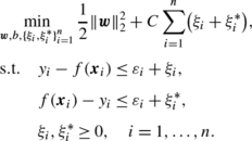
The primal optimization problem for the weighted SVR (WSVR) is defined by

where ϵ>0 is the insensitive-zone thickness. Note that, as in the classification case, WSVR is reduced to the original SVR when C _i =C for i=1,…,n. Thus, WSVR includes SVR as a special case.

The corresponding dual problem is given by

The final solution, i.e., the regression function $f:{\mathcal{X}}\rightarrow{\mathbb{R}}$, is in the following form:

The KKT conditions for the above dual problem are given as

(29a)

(29b)

(29c)

(29d)

Then the training instances can be partitioned into the following three index sets (see Fig. 12):

Fig. 12

Partitioning of data points in SVR

Let

Then, from (29a), (29b), (29c) and (29d) we obtain

where $\mathrm{diag}(\boldsymbol {s}_{{ \mathcal{O}}})$ indicates the diagonal matrix with diagonal elements given by $\boldsymbol {s}_{{ \mathcal{O}}}$. Because these functions are affine w.r.t. c, we can easily detect an event by monitoring the inequalities in (29a), (29b), (29c) and (29d). We can follow the solution path of SVR by using essentially the same technique as SVM classification (and thus the details are omitted).

5.1.2 Experiments on regression

As an application of WSVR, we consider a heteroscedastic regression problem, where output noise variance depends on input points. In heteroscedastic data modeling, larger (resp. smaller) weights are usually assigned to instances with smaller (resp. larger) variances. Because the point-wise variances are often unknown in practice, they should also be estimated from data. A standard approach is to alternately estimate the weight vector c based on the current WSVR solution and update the WSVR solutions based on the new weight vector c (Kersting et al. 2007).

We set the weights as

(30)

where $e_{i} = y_{i} - \widehat{f}(\boldsymbol {x}_{i})$ is the residual of the instance (x _i ,y _i ) from the current fit $\widehat{f}(\boldsymbol {x}_{i})$, and $\widehat{\sigma}$ is an estimate of the common standard deviation of the noise computed as $\widehat{\sigma} = \sqrt{\frac{1}{n}\sum_{i = 1}^{n} e_{i}^{2}}$. We employed the following procedure for the heteroscedastic data modeling:

• Step 1: Training WSVR with uniform weights (i.e., C _i =C ₀ for i=1,…,n.).

• Step 2: Update weights by (30) and update the solution of WSVR accordingly. Repeat this step until $\frac{1}{n} \sum_{i = 1}^{n}| (e^{(\mathrm{old})}_{i} - e_{i} ) / e^{(\mathrm{old})}_{i} |\leq10^{-3}$ holds, where e ^(old) is the previous training error.

We investigated the computational cost of Step 2. We applied the above procedure to the Boston housing data set. The sample size is 506 and the number of features is p=13. The inputs were normalized in [−1,1]^p. We randomly sampled n=404 instances for SVR training from the original data set, and the experiments were repeated 10 times. We used the Gaussian kernel (25) with γ∈{10,1,0.1}. The insensitive-zone thickness in WSVR was fixed to ε=0.05.

Each plot of Fig. 13 shows the average CPU time and standard error for C ₀∈{1,10,…,10⁴}, and Fig. 14 shows the number of repetitions performed in Step 2. This shows that our path-following approach is faster than the SMO algorithm especially for large C ₀.

Fig. 13

Comparison of CPU time for heteroscedastic modeling on the Boston housing data. The optimal C ₀ and γ in terms of the validation error (using the squared loss) are C ₀=10000 and γ=0.1

Fig. 14

The number of weight updates for the Boston housing data

5.2 Ranking

Recently, the problem of learning to rank has attracted wide interest as a challenging topic in machine learning and information retrieval (Liu 2009). Here, we focus on a method called the ranking SVM (RSVM) (Herbrich et al. 2000). RSVM learns a ranking model using a similar formulation to SVM. Arreola et al. (2008) derived the regularization path algorithm for RSVM. In this subsection, we describe that an instance-weighting strategy is useful in the ranking task and our solution path approach can be applied to the weighted variant of RSVM.

5.2.1 Formulation

Assume that we have a set of n triplets $\{(\boldsymbol {x}_{i}, y_{i}, q_{i})\}_{i = 1}^{n}$ where x _i ∈ℝ^p is a feature vector of an item and y _i ∈{r ₁,…,r _q } is a relevance of x _i to a query q _i . The relevance has an order of the preference r _q ≻r _q−1≻⋯≻r ₁, where r _q ≻r _q−1 means that r _q is preferred to r _q−1. The goal is to learn a ranking function f(x) that returns a larger value for a preferred item. More precisely, for items x _i and x _j such that q _i =q _j , we want the ranking function f(x) to satisfy

Let us define the following set of pairs:

RSVM solves the following optimization problem:

In practical ranking tasks such as information retrieval, it is natural that a pair of items with highly different preference levels has a larger weight than that with similar preference levels. Based on this prior knowledge, Cao et al. (2006) and Xu et al. (2006) proposed to assign different weights C _ij to different relevance pairs $(i, j) \in { \mathcal{P}}$. This is a cost-sensitive variant of RSVM whose primal problem is given as

Because this formulation is interpreted as a WSVM for pairs of items $(i, j) \in { \mathcal{P}}$, we can use our path approach. Note that the solution path algorithm for the cost-sensitive RSVM is regarded as an extension of Arreola et al. (2008), in which the solution path for the standard RSVM was studied.

Now, let us consider a model selection problem for the weighting pattern $\{C_{ij}\}_{(i, j) \in { \mathcal{P}}}$. We assume that the weighting pattern is represented as

(31)

where

(32)

(33)

and C ₀ is the common regularization parameter.² We follow the multi-parametric solution path from $\{C^{(\mathrm{old})}_{ij}\}_{(i, j) \in { \mathcal{P}}}$ to $\{C^{(\mathrm{new})}_{ij}\}_{(i, j) \in { \mathcal{P}}}$ and the best θ is selected based on the validation performance.

The performance of ranking algorithms is usually evaluated by some information-retrieval measures such as the normalized discounted cumulative gain (NDCG) (Järvelin and Kekäläinen 2000). Consider a query q and define q(j) as the index of the j-th largest item among $\{f(\boldsymbol {x}_{i})\}_{i \in\{i | q_{i} = q\}}$. The NDCG at position k for a query q is defined as

(34)

where Z is a constant to normalize the NDCG in [0,1]. Note that the NDCG value in (34) is defined using only the top k items and the rest are ignored. The NDCG for multiple queries are defined as the average of (34).

The goal of our model selection problem is to choose θ with the largest NDCG value. As explained below, we can identify θ that attains the exact maximum NDCG value for validation samples by exploiting the piecewise linearity of the solution path. The NDCG value changes only when there is a change in the top k ranking, and the rank of two items x _i and x _j changes only when f(x _i ) and f(x _j ) cross. Then change points of the NDCG can be exactly identified because f(x) changes in a piecewise-linear manner. Figure 15 schematically illustrates piecewise-linear paths and the corresponding NDCG path for validation samples. The validation NDCG changes in a piecewise-constant manner, and change points are found when there is a crossing between two piecewise-linear paths.

Fig. 15

The schematic illustration of the NDCG path. The upper plot shows outputs for 3 items which have different levels of preferences y. The bottom plot shows the changes of the NDCG. Since the NDCG depends on the sorted order of items, it changes only when two lines of the upper plot intersect

5.2.2 Experiments on ranking

We used the OHSUMED data set included in the LETOR package (version 3.0) provided by Microsoft Research Asia (Liu et al. 2007). We used the query-level normalized version of the data set containing 106 queries. The total number of query-document pairs is 16140, and the number of features is p=45. The data set provided is originally partitioned into 5 subsets, each of which has training, validation, and test sets for 5-fold cross validation. Here, we only used the training and the validation sets.

We compared the CPU time of our path algorithm and the SMO algorithm to change $\{C_{ij}\}_{(i,j) \in { \mathcal{P}}}$ from the flat weight pattern (32) to the relevance weight pattern (33). We need to modify the SMO algorithm to train the model without the explicit bias term b. The usual SMO algorithm updates two selected parameters per iteration to ensure that the solution satisfies the equality constraint derived from the optimality condition of b. Since RSVM has no bias term, the algorithm is adapted to update one parameter per iteration (Vogt 2002). We employed the update rule of Vogt (2002) to adapt the SMO algorithm to RSVM and we chose the maximum violating point as the parameter to update. This strategy is analogous to the maximum violating-pair working set selection of Keerthi et al. (2001) in ordinary SVM. Since it took relatively large computation time, we ran the SMO algorithm only at 10 points uniformly taken in $[C_{ij}^{(\mathrm{old})}, C_{ij}^{(\mathrm{new})}]$. We considered every pair of initial weight C ₀∈{10⁻⁵,…,10⁻¹} and Gaussian width γ∈{10,1,0.1}. The results, given in Fig. 16 (the average CPU time and its standard error), show that the path algorithm is faster than the SMO in all of the settings.

Fig. 16

CPU time comparison for RSVM. The optimal C ₀ and γ in terms of validation NDCG are C ₀=0.01 and γ=1

The CPU time of the path algorithm in Fig. 16(a) increases as C ₀ increases because the number of breakpoints and the size of the set ${\mathcal{M}}$ also increase. Since our path algorithm solves a linear system with size $|{ \mathcal{M}}|$ using $O(|{\mathcal{M}}|^{2})$ update in each iteration, practical computational time depends on $|{\mathcal{M}}|$ especially in large data sets. In the case of RSVM, the maximum value of $|{\mathcal{M}}|$ is the number of pairs of training documents $m = |{ \mathcal{P}}|$. For each fold of the OHSUMED data set, m=367663, 422716, 378087, 295814, and 283484. If $|{\mathcal{M}}| \approx m$, a large computational cost may be needed for updating the linear system. However, as Fig. 17 shows, the size $|{\mathcal{M}}|$ is at most about one hundred in this setup.

Fig. 17

The number of instances on the margin $|{\mathcal{M}}|$ in ranking experiment

Figure 18 shows the example of the path of validation NDCG@10. Since the NDCG depends on the sorted order of documents, direct optimization is rather difficult (Liu 2009). Using our path algorithm, however, we can detect the exact behavior of the NDCG by monitoring the change of scores f(x) in the validation data set. Then we can find the best weighting pattern by choosing θ with the maximum NDCG for the validation set.

Fig. 18

The change of NDCG@10 for γ=0.1 and C=0.01. The parameter θ in the horizontal axis is used as c ^(old)+θ(c ^(new)−c ^(old))

5.3 Transduction

In transductive inference (Vapnik 1995), we are given unlabeled instances along with labeled instances. The goal of transductive inference is not to estimate the true decision function, but to classify the given unlabeled instances correctly. The transductive SVM (TSVM) (Joachims 1999) is one of the most popular approaches to transductive binary classification. The objective of the TSVM is to maximize the classification margin for both labeled and unlabeled instances.

5.3.1 Formulation

Suppose we have k unlabeled instances $\{ \boldsymbol {x}_{i}^{*} \}_{i=1}^{k}$ in addition to n labeled instances $\{ (\boldsymbol {x}_{i}, y_{i}) \}_{i=1}^{n}$. The optimization problem of TSVM is formulated as

(35)

where C and C ^∗ are the regularization parameters for labeled and unlabeled data, respectively, and $y^{*}_{j} \in\{-1, +1\}, j = 1, \ldots, k$, are the labels of the unlabeled instances $\{ \boldsymbol {x}_{i}^{*} \}_{i=1}^{k}$. Note that (35) is a combinatorial optimization problem with respect to $\{ y_{j}^{*} \}_{j \in\{ 1, \ldots, k \}}$. The optimal solution of (35) can be found if we solve binary SVMs for all possible combinations of $\{y_{j}^{*}\}_{j \in\{1,\ldots,k\}}$, but this is computationally intractable even for moderate k. To cope with this problem, Joachims (1999) proposed an algorithm that approximately optimizes (35) by solving a series of WSVMs. The subproblem is formulated by assigning temporarily estimated labels $\widehat{y}_{j}^{*}$ to unlabeled instances:

(36)

where $C_{-}^{*}$ and $C_{+}^{*}$ are the weights for unlabeled instances $\{j \mid\widehat{y}_{j}^{*} = -1 \}$ and $\{j \mid\widehat{y}_{j}^{*} = +1 \}$, respectively. The entire algorithm is given as follows (see Joachims 1999, for details):

Step 1::

Set the parameters C, C ^∗, and k ⁺, where k ⁺ is defined as

k ⁺ is defined so that the balance of positive and negative instances in the labeled set is equal to that in the unlabeled set.

Step 2::

Optimize the decision function using only the labeled instances and compute the decision function values $\{f(\boldsymbol {x}_{j}^{*})\}_{j=1}^{k}$. Assign the positive label $y_{j}^{*} = 1$ to the top k ⁺ unlabeled instances in decreasing order of $f(\boldsymbol {x}_{j}^{*})$, and the negative label $y_{j}^{*} = -1$ to the remaining instances. Set $C_{-}^{*}$ and $C_{+}^{*}$ to some small values (see Joachims 1999, for details).

Step 3::

Train SVM using all the instances (i.e., solve (36)). Switch the labels of a pair of positive and negative unlabeled instances if the objective value (35) is reduced, where the pair of instances is selected based on $\{\xi_{j}^{*}\}_{j \in\{1,\ldots,k\}}$ (see Joachims 1999, for details). Iterate this step until no data pair decreases the objective value.

Step 4::

Set $C_{-}^{*}=\min(2 C_{-}^{*}, C^{*})$ and $C_{+}^{*}=\min(2C_{+}^{*}, C^{*})$. If $C_{-}^{*} \geq C^{*}$ and $C_{+}^{*} \geq C^{*}$, terminate the algorithm. Otherwise return to Step 3.

Our path-following algorithm can be applied to Steps 3 and 4 for accelerating the above TSVM algorithm. Step 3 can be carried out via path-following as follows:

Step 3(a):

Choose a pair of positive instance $\boldsymbol {x}_{m}^{*}$ and negative instance $\boldsymbol {x}_{m'}^{*}$.

Step 3(b):

After removing the positive instance $\boldsymbol {x}_{m}^{*}$ by decreasing its weight parameter C _m from $C_{+}^{*}$ to 0, add the instance $\boldsymbol {x}_{m}^{*}$ as a negative one by increasing C _m from 0 to $C_{-}^{*}$.

Step 3(c):

After removing the negative instance $\boldsymbol {x}_{m'}^{*}$ by decreasing its weight parameter C _m′ from $C_{-}^{*}$ to 0, add the instance $\boldsymbol {x}_{m'}^{*}$ as a positive one by increasing C _m′ from 0 to $C_{+}^{*}$.

Note that the label switching in Steps 3(b) and 3(c) may be merged into a single step. Step 4 also can be carried out by our path-following algorithm.

5.3.2 Experiments on transduction

We compare the computation time of the proposed path-following algorithm and the SMO algorithm for Steps 3 and 4 of the TSVM algorithm. We used the spam data set obtained from the UCI machine learning repository (Asuncion and Newman 2007). The sample size is 4601, and the number of features is p=57. We randomly selected 10 % of data points as labeled instances, and the remaining 90 % were used as unlabeled instances. The inputs were normalized in [0,1]^p.

Figure 19 shows the average CPU time and its standard error over 10 runs for the Gaussian width γ∈{10,1,0.1} and C∈{1,10,10²,…,10⁴}. The figure shows that our algorithm is consistently faster than the SMO algorithm in all of these settings.

Fig. 19

CPU time comparison for the transductive SVM. The optimal C ₀ and γ in terms of the classification error for the unlabeled data instances (using the 0-1 loss) are C ₀=1000 and γ=1

6 Discussion and conclusion

In this paper, we developed an algorithm for updating solutions of instance-weighted SVMs. Our algorithm was built upon multiple parametric programming techniques, and it is an extension of existing single-parameter path-following algorithms to multiple parameters. We experimentally demonstrated the computational advantage of the proposed algorithm on a wide range of applications including on-line time-series analysis, heteroscedastic data modeling, covariate shift adaptation, ranking, and transduction.

Another important advantage of the proposed approach beyond the computational efficiency is that the exact solution path is represented in a piecewise linear form. In SVM (and its variants), the decision function f(x) also has a piecewise linear form because f(x) is linear in the parameters α and b. This enables us to compute the entire path of the validation error and to select the model with the minimum validation error. Let ${ \mathcal{V}}$ be the validation set and the validation loss is defined as $\sum_{i \in { \mathcal{V}}} \ell(y_{i}, f(\boldsymbol {x}_{i}))$. Suppose that the current weight is expressed as c+θ d in a critical region ${ \mathcal{R}}$ using a parameter θ∈ℝ, and the output has the form f(x _i )=a _i θ+b _i for some scalar constants a _i and b _i . Then the minimum validation error in the current critical region ${ \mathcal{R}}$ can be identified by solving the following optimization problem:

(37)

After following the entire solution-path, the best model can be selected among the candidates in the finite number of critical regions. In the case of the 0-1 loss, i.e.,

the problem (37) can be solved by monitoring all the points at which f(x _i )=0 (see Fig. 6). Furthermore, if the validation error is measured by the squared loss

the problem (37) can be analytically solved in each critical region. As another interesting example, we described how to find the maximum validation NDCG in a ranking problem (see Sect. 5.2). In the case of NDCG, the problem (37) can be solved by monitoring all the intersections of f(x _i ) and f(x _j ) such that y _i ≠y _j (see Fig. 15).³

Although we focused only on quadratic programming (QP) machines in this paper, similar algorithms can be developed for linear programming (LP) machines. It is well-known in the parametric programming literature that the solution of LP and QP have a piecewise linear form if a linear function of hyper-parameters appears in the constant term of the constraints and/or the linear part of the objective function (see Ritter 1984; Best 1982; Gal 1995; Pistikopoulos et al. 2007, for more details). Indeed, the parametric LP technique (Gal 1995) has already been applied to several machine learning problems (Zhu et al. 2004; Yao and Lee 2007; Li and Zhu 2008). One of our future works is to apply the multi-parametric approach to these LP machines.

In this paper, we studied the changes of instance weights of various types of SVMs. There are many other situations in which a path of multiple hyper-parameters can be exploited. For instance, the application of the multi-parametric path approach to the following problems would be interesting future works:

• Different (functional) margin SVM:

  

  where δ _i ∈ℝ is a margin rescaling parameter. Chapelle and Keerthi (2010) indicated that this type of parametrization can be used to give different costs to each pair of items in ranking SVM.

• SVR with different insensitive-zone thickness. Although usual SVR has the common insensitive-zone thickness ε for all instances, different thickness ε _i for every instance can be assigned:

  

  In the case of common thickness, the optimal ε is known to be asymptotically proportional to the noise variance (Smola et al. 1998; Kwok and Tsang 2003). In the case of heteroscedastic noise, it would be reasonable to set different ε _i , each of which is proportional to the variance of each (iteratively estimated) y _i .

• The weighted lasso. The lasso solves the following quadratic programming problem (Tibshirani 1996):

  

  where λ is the regularization parameter. A weighted version of the lasso has been considered in Zou (2006):⁴

  

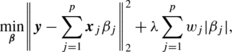
  where w _j is an individual weight parameters for each β _j . The weights are adaptively determined by $w_{j} = |\hat{\beta}_{j}|^{-\gamma}$, where $\hat{\beta}_{j}$ is an initial estimate of β _j and γ>0 is a parameter. A similar weighted parameter-minimization problem has also been considered in Candes et al. (2008) in the context of signal reconstruction. They considered the following weighted ℓ ₁-minimization problem:⁵

  

  where y∈ℝ^m, Φ∈ℝ^m×n, and m<n. The goal of this problem is to reconstruct a sparse signal x from the measurement vector y and sensing matrix Φ. The constraint linear equations have infinitely many solutions and the simplest explanation of y is desirable. To estimate better sparse representation, they proposed an iteratively re-weighting strategy for estimating w _i .

In order to apply the multi-parametric approach to these problems, we need to determine the search direction of the path in the multi-dimensional hyper-parameter space. In many situations, search directions can be estimated from data.

Incremental-decremental SVM (Cauwenberghs and Poggio 2001; Martin 2002; Ma and Theiler 2003; Laskov et al. 2006; Karasuyama and Takeuchi 2009) exploits the piecewise linearity of the solutions. It updates SVM solutions efficiently when instances are added or removed from the training set. The incremental and decremental operations can be implemented using our instance-weight path approach. If we want to add an instance (x _i ,y _i ), we increase C _i from 0 to some specified value. Conversely, if we want to remove an instance (x _j ,y _j ), we decrease C _j to 0. The paths generated by these two approaches are different in general. The instance-weight path keeps the optimality of all the instances including currently added and/or removed ones. On the other hand, the incremental-decremental algorithm does not satisfy the optimality of adding and/or removing ones until the algorithm terminates. When we need to guarantee the optimality at intermediate points on the path, our approach is more useful.

In the parametric programming approach, numerical instabilities sometimes cause computational difficulty. In practical implementation, we usually update several quantities such as α, b, yf(x _i ), and L from the previous values without calculating them from scratch. However, the rounding error may be accumulated at every breakpoints. We can avoid such accumulation using the refresh strategy: re-calculating variables from scratch, for example, every 100 steps (note that, in this case, we need $O(n |{\mathcal{M}}|^{2})$ computations in every 100 steps). Fortunately, such numerical instabilities rarely occurred in our experiments, and the accuracy of the KKT conditions of the solutions were kept high enough.

Another (but related) numerical difficulty arises when the matrix M in (17) is close to singular. Wang et al. (2008) pointed out that if the matrix is singular, the update is no longer unique. To the best of our knowledge, this degeneracy problem is not fully solved in path-following literature. Many heuristics are proposed to circumvent the problem, and we used one of them in the experiments: adding a small positive constant to the diagonal elements of the kernel matrix. Other strategies are also discussed in Wu et al. (2008), Gärtner et al. (2009), and Ong et al. (2010).

Scalability of our algorithm depends on the size of ${ \mathcal{M}}$ because a linear system with $|{ \mathcal{M}}|$ unknowns must be solved at each breakpoint. Although we can update the Cholesky factor by the $O(|{ \mathcal{M}}|^{2})$ cost from the previous one, iterative methods such as conjugate gradients may be more efficient than the direct matrix update when $|{ \mathcal{M}}|$ is fairly large. When $|{ \mathcal{M}}|$ is small, the parametric programming approach can be applied to relatively large data sets, for example, the ranking experiments in Sect. 5.2 contain more than tens of thousands of instances.

References

Albert, A. (1972). Regression and the Moore-Penrose pseudoinverse. New York: Academic Press.
Allgower, E. L., & Georg, K. (1993). Continuation and path following. Acta Numerica, 2, 1–64.
Aronszajn, N. (1950). Theory of reproducing kernels. Transactions of the American Mathematical Society, 68, 337–404.
Arreola, K. Z., Gärtner, T., Gasso, G., & Canu, S. (2008). Regularization path for ranking SVM. In Proceedings of ESANN 2008, 16th European symposium on artificial neural networks, April 23–25, 2008, Bruges, Belgium (pp. 415–420).
Asuncion, A., & Newman, D. (2007). UCI machine learning repository. http://www.ics.uci.edu/~mlearn/MLRepository.html.
Bach, F., Heckerman, D., & Horvitz, E. (2006). Considering cost asymmetry in learning classifiers. Journal of Machine Learning Research, 7, 1713–1741.
Bennett, K. P., & Bredensteiner, E. J. (1997). A parametric optimization method for machine learning. INFORMS Journal on Computing, 9(3), 311–318.
Best, M. J. (1982). An algorithm for the solution of the parametric quadratic programming problem (Technical Report 82–24). Faculty of Mathematics, University of Waterloo.
Bickel, S., Bogojeska, J., Lengauer, T., & Scheffer, T. (2008). Multi-task learning for HIV therapy screening. In A. McCallum & S. Roweis (Eds.), Proceedings of 25th annual international conference on machine learning (ICML2008) (pp. 56–63).
Bland, R. G. (1977). New finite pivoting rules for the simplex method. Mathematics of Operations Research, 2, 103–107.
Boser, B. E., Guyon, I. M., & Vapnik, V. N. (1992). A training algorithm for optimal margin classifiers. In D. Haussler (Ed.), Proceedings of the fifth annual ACM workshop on computational learning theory (pp. 144–152). New York: ACM.
Boyd, S., & Vandenberghe, L. (2004). Convex optimization. Cambridge: Cambridge University Press.
Burde, W., & Blankertz, B. (2006). Is the locus of control of reinforcement a predictor of brain-computer interface performance. In Proceedings of the 3rd international brain-computer interface workshop and training course 2006, Graz, Austria. Graz: Verlag der Technischen Universität.
Candes, E., Wakin, M., & Boyd, S. (2008). Enhancing sparsity by reweighted ℓ 1 minimization. The Journal of Fourier Analysis and Applications, 14(5–6), 877–905.
Cao, L., & Tay, F. (2003). Support vector machine with adaptive parameters in financial time series forecasting. IEEE Transactions on Neural Networks, 14(6), 1506–1518.
Cao, Y., Xu, J., Liu, T.-Y., Li, H., Huang, Y., & Hon, H.-W. (2006). Adapting ranking SVM to document retrieval. In SIGIR’06: Proceedings of the 29th annual international ACM SIGIR conference on research and development in information retrieval (pp. 186–193). New York: ACM.
Cauwenberghs, G., & Poggio, T. (2001). Incremental and decremental support vector machine learning. In T. K. Leen, T. G. Dietterich, & V. Tresp (Eds.), Advances in neural information processing systems (pp. 409–415). Cambridge: MIT Press.
Chang, C.-C., & Lin, C.-J. (2011). LIBSVM: A library for support vector machines. ACM Transactions on Intelligent Systems and Technology, 2(3), 27. Software available at http://www.csie.ntu.edu.tw/~cjlin/libsvm.
Chapelle, O., & Keerthi, S. (2010). Efficient algorithms for ranking with SVMs. Information Retrieval, 13(3), 201–215.
Chen, W.-H., Shih, J.-Y., & Wu, S. (2006). Comparison of support-vector machines and back propagation neural networks in forecasting the six major Asian stock markets. International Journal of Electronic Finance, 1(1), 49–67.
Cortes, C., & Vapnik, V. (1995). Support-vector networks. Machine Learning, 20, 273–297.
DeCoste, D., & Wagstaff, K. (2000). Alpha seeding for support vector machines. In Proceedings of the international conference on knowledge discovery and data mining (pp. 345–359).
Dornhege, G., Millán, J., Hinterberger, T., McFarland, D., & Müller, K.-R. (Eds.) (2007). Toward brain computer interfacing. Cambridge: MIT Press.
Efron, B., Hastie, T., Johnstone, L., & Tibshirani, R. (2004). Least angle regression. Annals of Statistics, 32(2), 407–499.
Fine, S., & Scheinberg, K. (2002). Incremental learning and selective sampling via parametric optimization framework for SVM. In T. G. Dietterich, S. Becker, & Z. Ghahramani (Eds.), Advances in neural information processing systems (p. 14). Cambridge: MIT Press.
Gal, T. (1995). Postoptimal analysis, parametric programming, and related topics. Berlin: de Gruyter.
Gal, T., & Nedoma, J. (1972). Multiparametric linear programming. Management Science, 18(7), 406–422.
Gärtner, B., Giesen, J., Jaggi, M., & Welsch, T. (2009). A combinatorial algorithm to compute regularization paths. arXiv cs.LG.
Golub, G. H., & Van Loan, C. F. (1996). Matrix computations. Baltimore: Johns Hopkins University Press.
Gunter, L., & Zhu, J. (2007). Efficient computation and model selection for the support vector regression. Neural Computation, 19(6), 1633–1655.
Hastie, T., Rosset, S., Tibshirani, R., & Zhu, J. (2004). The entire regularization path for the support vector machine. Journal of Machine Learning Research, 5, 1391–1415.
Herbrich, R., Graepel, T., & Obermayer, K. (2000). Large margin rank boundaries for ordinal regression. In A. Smola, P. Bartlett, B. Schölkopf, & D. Schuurmans (Eds.), Advances in large margin classifiers (pp. 115–132). Cambridge: MIT Press.
Järvelin, K., & Kekäläinen, J. (2000). IR evaluation methods for retrieving highly relevant documents. In SIGIR’00: Proceedings of the 23rd annual international ACM SIGIR conference on research and development in information retrieval (pp. 41–48). New York: ACM.
Jiang, J., & Zhai, C. (2007). Instance weighting for domain adaptation in NLP. In Proceedings of the 45th annual meeting of the association for computational linguistics (pp. 264–271).
Joachims, T. (1999). Transductive inference for text classification using support vector machines. In Proceedings of the 16th annual international conference on machine learning (ICML 1999) (pp. 200–209). San Francisco: Morgan Kaufmann.
Kanamori, T., Hido, S., & Sugiyama, M. (2009). A least-squares approach to direct importance estimation. Journal of Machine Learning Research, 10, 1391–1445.
Karasuyama, M., & Takeuchi, I. (2009). Multiple incremental decremental learning of support vector machines. In Y. Bengio, D. Schuurmans, J. Lafferty, C. K. I. Williams, & A. Culotta (Eds.), Advances in neural information processing systems (Vol. 22, pp. 907–915).
Keerthi, S., Shevade, S., Bhattacharyya, C., & Murthy, K. (2001). Improvements to Platt’s SMO algorithm for SVM classifier design. Neural Computation, 13(3), 637–649.
Kersting, K., Plagemann, C., Pfaff, P., & Burgard, W. (2007). Most likely heteroscedastic Gaussian process regression. In Z. Ghahramani (Ed.), Proceedings of the 24th annual international conference on machine learning (ICML 2007) (pp. 393–400). Madison: Omnipress.
Kwok, J., & Tsang, I. (2003). Linear dependency between ε and the input noise in ε-support vector regression. IEEE Transactions on Neural Networks, 14(3), 544–553.
Laskov, P., Gehl, C., Kruger, S., & Müller, K.-R. (2006). Incremental support vector learning: Analysis, implementation and applications. Journal of Machine Learning Research, 7, 1909–1936.
Lee, G., & Scott, C. (2007). The one class support vector machine solution path. In ICASSP, IEEE international conference on acoustics, speech and signal processing—proceedings (Vol. 2, pp. II521–II524).
Li, Y., & Zhu, J. (2008). l 1-norm quantile regression. Journal of Computational and Graphical Statistics, 17(1), 163–185.
Lin, C.-F., & Wang, S.-D. (2002). Fuzzy support vector machines. IEEE Transactions on Neural Networks, 13(2), 464–471.
Lin, Y., Lee, Y., & Wahba, G. (2002). Support vector machines for classification in nonstandard situations. Machine Learning, 46(1/3), 191–202.
Liu, T.-Y. (2009). Learning to rank for information retrieval. Foundations and Trends in Information Retrieval, 3(3), 225–331.
Liu, T. Y., Xu, J., Qin, T., Xiong, W., & Li, H. (2007). LETOR: Benchmark dataset for research on learning to rank for information retrieval. In SIGIR’07: Proceedings of the learning to rank workshop in the 30th annual international ACM SIGIR conference on research and development in information retrieval.
Ma, J., & Theiler, J. (2003). Accurate online support vector regression. Neural Computation, 15(11), 2683–2703.
Martin, M. (2002). On-line support vector machines for function approximation (Technical report). Software Department, University Politecnica de Catalunya.
Mattera, D., & Haykin, S. (1999). Support vector machines for dynamic reconstruction of a chaotic system. In B. Scholkopf, C. J. Burges, & A. J. Smola (Eds.), Advances in kernel methods: support vector learning (pp. 211–241). Cambridge: MIT Press.
Müller, K.-R., Smola, A. J., Rätsch, G., Schökopf, B., Kohlmorgen, J., & Vapnik, V. (1999). Using support vector machines for time series prediction. In Advances in kernel methods: support vector learning (pp. 243–253). Cambridge: MIT Press.
Murata, N., Kawanabe, M., Ziehe, A., Müller, K.-R., & Amari, S. (2002). On-line learning in changing environments with applications in supervised and unsupervised learning. Neural Networks, 15(4–6), 743–760.
Ong, C.-J., Shao, S., & Yang, J. (2010). An improved algorithm for the solution of the regularization path of support vector machine. IEEE Transactions on Neural Networks, 21(3), 451–462.
Pistikopoulos, E. N., Georgiadis, M. C., & Dua, V. (2007). Process systems engineering, volume 1, multi-parametric programming. New York: Wiley.
Platt, J. C. (1999). Fast training of support vector machines using sequential minimal optimization. In B. Schölkopf, C. J. C. Burges, & A. J. Smola (Eds.), Advances in kernel methods—support vector learning (pp. 185–208). Cambridge: MIT Press.
Raina, R., Battle, A., Lee, H., Packer, B., & Ng, A. (2007). Self-taught learning: transfer learning from unlabeled data. In Z. Ghahramani (Ed.), Proceedings of the 24th annual international conference on machine learning (ICML 2007) (pp. 759–766). Madison: Omnipress.
Ritter, K. (1984). On parametric linear and quadratic programming problems. In R. Cottle, M. L. Kelmanson, & B. Korte (Eds.), Mathematical programming: proceedings of the international congress on mathematical programming (pp. 307–335). Amsterdam: Elsevier.
Rosset, S. (2009). Bi-level path following for cross validated solution of kernel quantile regression. Journal of Machine Learning Research, 10, 2473–2505.
Rosset, S., & Zhu, J. (2007). Piecewise linear regularized solution paths. Annals of Statistics, 35, 1012–1030.
Schott, J. R. (2005). Matrix analysis for statistics. New York: Wiley-Interscience.
Shimodaira, H. (2000). Improving predictive inference under covariate shift by weighting the log-likelihood function. Journal of Statistical Planning and Inference, 90(2), 227–244.
Sjostrand, K., Hansen, M., Larsson, H., & Larsen, R. (2007). A path algorithm for the support vector domain description and its application to medical imaging. Medical Image Analysis, 11(5), 417–428.
Smola, A. J., Murata, N., Schölkopf, B., & Müller, K.-R. (1998). Asymptotically optimal choice of ε-loss for support vector machines. In L. Niklasson, M. Bodén, & T. Ziemke (Eds.), Proceedings of the international conference on artificial neural networks (pp. 105–110). Berlin: Springer.
Sugiyama, M., Krauledat, M., & Müller, K.-R. (2007). Covariate shift adaptation by importance weighted cross validation. Journal of Machine Learning Research, 8, 985–1005.
Takeuchi, I., Le, Q. V., Sears, T. D., & Smola, A. J. (2006). Nonparametric quantile estimation. Journal of Machine Learning Research, 7, 1231–1264.
Takeuchi, I., Nomura, K., & Kanamori, T. (2009). Nonparametric conditional density estimation using piecewise-linear solution path of kernel quantile regression. Neural Computation, 21(2), 533–559.
Tibshirani, R. (1996). Regression shrinkage and selection via the lasso. Journal of the Royal Statistical Society. Series B. Statistical Methodology, 58(1), 267–288.
Vapnik, V., Golowich, S. E., & Smola, A. (1996). Support vector method for function approximation, regression estimation, and signal processing. In M. Mozer, M. Jordan, & T. Petsche (Eds.), Advances in neural information processing systems (Vol. 9, pp. 281–287). Cambridge: MIT Press.
Vapnik, V. N. (1995). The nature of statistical learning theory. Berlin: Springer.
Vogt, M. (2002). SMO algorithms for support vector machines without bias term (Technical report). Technische Universität Darmstadt.
Wang, G., Yeung, D.-Y., & Lochovsky, F. H. (2008). A new solution path algorithm in support vector regression. IEEE Transactions on Neural Networks, 19(10), 1753–1767.
Wu, Z., Zhang, A., & Li, C. (2008). Trace solution paths for SVMs via parametric quadratic programming. In KDD Workshop report DMMT’08 data mining using matrices and tensors.
Xu, J., Cao, Y., Li, H., & Huang, Y. (2006). Cost-sensitive learning of SVM for ranking. In J. Fürnkranz, T. Scheffer, & M. Spiliopoulou (Eds.), Machine learning: ECML 2006, Proceedings of 17th European conference on machine learning, Berlin, Germany, September 18–22, 2006 (Vol. 4212, pp. 833–840). Berlin: Springer.
Yang, X., Song, Q., & Wang, Y. (2007). A weighted support vector machine for data classification. International Journal of Pattern Recognition and Artificial Intelligence, 21(5), 961–976.
Yao, Y., & Lee, Y. (2007). Another look at linear programming for feature selection via methods of regularization (Technical Report 800). Department of Statistics, The Ohio State University.
Zhu, J., Rosset, S., Hastie, T., & Tibshirani, R. (2004). 1-norm support vector machines. In S. Thrun, L. Saul, & B. Schölkopf (Eds.), Advances in neural information processing systems (Vol. 16). Cambridge: MIT Press.
Zou, H. (2006). The adaptive lasso and its oracle properties. Journal of the American Statistical Association, 101(476), 1418–1429.
Acknowledgements
The authors would like to thank the anonymous referees and the action editor for suggesting improvements in this paper. This work was supported by Grant-in-Aid for JSPS Fellows (No. 00008773) and the FIRST program.
Author information
Authors and Affiliations
Corresponding author
Additional information
Editor: Thorsten Joachims.
Rights and permissions
About this article
Cite this article
Karasuyama, M., Harada, N., Sugiyama, M. et al. Multi-parametric solution-path algorithm for instance-weighted support vector machines. Mach Learn 88, 297–330 (2012). https://doi.org/10.1007/s10994-012-5288-5
Received:
Accepted:
Published:
Issue Date:
DOI: https://doi.org/10.1007/s10994-012-5288-5