What is climate? What is a model? How do we describe the uncertainty in a model? This chapter introduces key terms and concepts. We start with basic definitions of climate and weather. Then, we discuss models. Even if we do not realize it, we use models all the time. So we describe a few different conceptual types of models and put climate models in context. Finally we introduce the concept of uncertainty. As we discuss later in the book, models may have errors and still be useful, but this requires understanding the errors (the uncertainties) and understanding where they come from. These concepts are common to many types of modeling.
In order to describe climate modeling and the climate system, it is necessary to have a common conception of exactly what we are trying to simulate, and what a model actually is. What is climate? What is a model? How do we measure the uncertainty in a model? This chapter introduces some key terms and concepts. We start with some basic definitions of climate and weather. Everyone will come to this book with a preconceived definition of what climate and weather are, but separating these concepts is important for understanding how modeling of climate and weather are similar and why they are different. It also makes sense to discuss what a model is. Even if we do not realize it, we use models all the time. So we describe a few different conceptual types of models and put climate models in context. Finally we introduce the concept of uncertainty. As we discuss later in the book, models may have errors and still be useful, but this requires understanding the errors (the uncertainties) and understanding where they come from. Most of these concepts are common to many types of modeling, and we provide examples throughout the text.
1.1 What Is Climate?
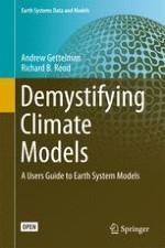
Climate is perhaps easiest to explain as the distribution of possible weather states. On any given day and in any given place, the history of weather events can be compiled into a distribution with probabilities of what the weather might be (see Fig. 1.1). This figure is called a probability distribution function, representing a probability distribution.1 The horizontal axis represents a value (e.g., temperature), and the vertical axis represents the probability (or frequency of occurrence) of that event’s (i.e., a given temperature) occurring or having occurred. If based on observations, then the frequency can be the number of times a given temperature occurs. The higher the line, the more probable the event. The most frequent occurrence is the highest probability (the mode). The total area under the line is the probability. If the total area is given a value of 1, then the area under each part of the curve is the fractional chance that an event exceeding some threshold will occur. In Fig. 1.1, the area to the right of point T1 is the probability that the temperature will be greater than T1, which might be about 20 % of the curve. The mean, or expected value, is the weighted average of the points. It need not be the point with the highest frequency. The mean value is the point at which half the probability (50 %) is on one side of the mean, and half on the other. The median is the value at which half the points are on one side and half on the other.
Fig. 1.1
A probability distribution function with the value on the horizontal axis, and the frequency of occurrence on the vertical axis
×
Anzeige
Here is an important and obvious question: How can we predict the climate (for next season, next year, or 50 years from now) if we cannot predict the weather (in 5 or 10 days)? The answer is, we use probability: The climate is the distribution of probable weather. The weather is a particular location in that distribution, and it is conditional on the current state of the system. The chance of a hurricane hitting Miami next week depends mostly on whether one has formed or is forming, and if one has formed, whether it is heading in the direction of Miami. As another example, the chance of having a rainy day in Seattle in January is high. But, given a particular day in January, with a weather state that might be pushing storms well to the north or south, the probability of rain the next day might be very low. In 50 Januaries, though, the probability of rain would be high. So climate is the distribution of weather (sometimes unknown). Weather is a given state in that distribution (often uncertain).
In a probability distribution of climate, the probabilities and the curve change over time: In the middle latitudes, the chance of snow is higher in winter than in summer. The curves will look different from place to place: Some climates have narrow distributions (see Fig. 1.2a), which means the weather is often very close to the average. Think about Hawaii, where the average of the daily highs and lows do not change much over the course of the year or Alaska, where the daily highs and lows may be the same as in Hawaii in summer, but not in winter. For Alaska the annual distribution of temperature is a very broad distribution (more like Fig. 1.2b). Of course, even in Hawaii, extreme events occur. For a distribution like precipitation, which is bounded at one end by zero (no precipitation) the distribution might be “skewed” (Fig. 1.2c) with a low frequency of high events marking the ‘extreme’. As events are more extreme (think about hurricanes like Katrina or Sandy), there are fewer such events in the historical record. There may even be possible extreme events that have not occurred. So our description of climate is incomplete or uncertain. This is particularly true for rare (low-probability) events. These events are also the events that cause the most damage.
Fig. 1.2
Different probability distribution functions: a narrow, b wide and c skewed distributions
×
One aspect of shifting distributions is that extremes can change a lot more than the mean value (see Fig. 1.3). The mean is the value at which the area is equal on each side of the distribution. The mean is the same as the median if the distribution is symmetric. Simply moving the distribution to the right or left causes the area (meaning, the probability) beyond some fixed threshold to increase (or decrease). If the curve represents temperature, then shifting it to warmer temperatures (Fig. 1.3a) decreases the chance of cold events and really increases the chance of warm events. But note that some cold events still occur. Also, you can change the distribution without changing the mean by making the distribution wider (or broader). The mathematical term for the width of a distribution is variance, a statistical term for variability. This situation is illustrated in Fig. 1.3b. The mean is unchanged in Fig. 1.3b, but the chance of exceeding a given threshold for warm or cold temperatures changes. In other words, the climate (particularly a climate extreme) changes dramatically, even if the mean stays the same. The change need not be symmetric: Hot may change more than cold (or vice versa). Figure 1.3c is not a symmetric distribution. The key is to see climate as the distribution, not as a fixed number (often the mean).
Fig. 1.3
Shifting probability distribution functions are illustrated in different ways going from the blue to red distribution. The thick lines are the distribution, the thin dashed lines are the mean of the distributions and the dotted lines are fixed points to illustrate probability. Shown is a increase in mean, b increase in variance (width), c increase in mean and variance
×
This brings us to the fundamental difference between weather and climate forecasting. In weather forecasting,2 we need to know the current state of the system and have a model for projecting it forward. Often the model can be simple. One “model” we all use is called persistence: What is the weather now? It may be like that tomorrow. In many places (e.g., Hawaii), such a model is not bad, but sometimes it is horribly wrong (e.g., when a hurricane hits Hawaii). So we try to use more sophisticated models, now typically numerical ones. These models go by the name numericalweather prediction (NWP) models, and they are used to “forecast” the evolution of the earth system from its current state.
Anzeige
Climate forecasting uses essentially the same type of model. But the goal of climate forecasting is to characterize the distribution. This may mean running the model for a long time to describe the distribution of all possible weather states correctly. If you start up a weather model from two different states (two different days), you hope to get a different answer each time. But for climate, you want to get the same distribution (the same climate), regardless of when the model started. We return to these examples again later.
1.2 What Is a Model?
A model, in essence, is a representation of a system. A model can be physical (building blocks) or abstract (an image on paper like a plan, or in your head). Abstract models can also be mathematical (monetary or physical totals in a spreadsheet). Ordinary physics that describes how cars go (or, more importantly, how they stop suddenly) is a model for how the physical world behaves. Numbers themselves are abstract models. A financial statement is a model of the money and resource flows of a household, corporation or country. Models are all around us, and we use them to abstract, make tractable and understand our human and natural environment.
As a concrete example, think about different “models” of a building. There can be many types of models of a building. A physical model of the building would usually be at a smaller scale that you can hold in your hand. There are several different abstract models of a building, and they are used for different purposes. Architects and engineers produce building plans: two-dimensional representations of the building, used to construct and document the building. Some of these are highly detailed drawings of specific parts of the building, such as the exterior, or the electrical and plumbing systems. The engineer may have built not just a physical model of the building, but perhaps even a more detailed structural model designed to understand how the building will react to wind or ground motion (earthquakes). Increasingly, these models are “virtual”: The structure is simulated on a computer.
We are familiar with all these sorts of model, but there are other more abstract models that deal with flows and budgets of materials or money. The owner and builder also probably have a spreadsheet model of the costs of construction of the building. This financial model is not certain, because it is really an estimate (or forecast, see below) of all the different costs of construction. And, finally, the owner likely has another model of the financial operation of the building: the money borrowed to finance the building, any income from a commercial building, and the costs of maintenance and operations of the building. The operating plan is really a projection into the future: It depends on a lot of uncertainties, like the cost of electricity or the value of the income from a building. The projection depends on these inputs, which the spreadsheet does not try to predict. The prediction is conditional on the inputs.
Models All Around Us
Models are everywhere in our world. Many models are familiar and physical, such as a small-scale model of a building or a bridge, or a mockup of a satellite or an airplane. Some models we use every day are made up of numbers. Many people use a model with numbers to manage income and expenses, savings and debts; that is, a budget. When the model of a bridge is placed in a computer-assisted design program, or a financial budget is put into a spreadsheet on a personal computer, then one has a “numerical” model. These models have a set of mathematical equations that behave with a specific set of rules, principles or laws.
Climate models are numerical models that calculate budgets of mass, momentum (velocity) and energy based on the physical laws of conservation. For example, energy is conserved (neither created or destroyed) and can, therefore, be counted. The physical laws on which climate models are based are discussed in more detail in Chap. 4. Weather and climate are dynamical systems; that is, they evolve over time. We rely on models of dynamical systems for many aspects of modern life. Here we illustrate a few examples of models that affect our everyday lives.
Climate models are closely related to weather forecast models; both simulate how fluids (air or water) move and interact, and how they exchange heat. An obvious example of a model that affects daily life is the weather forecast model, which is used in planning by individuals, governments, corporations and finance. The exact same physical principles of fluid flow are used to simulate a process in a chemical plant that takes different substances as liquids or gasses, reacts them together under controlled temperature and pressure, and produces new substances. Water and sewage treatment plants share similar principles and models. Internal combustion engines used for cars, trucks, ships and power plants are developed using models to understand how fuel enters the engine and produces heat, and that heat produces motion. Airplanes are also developed using modeling of the airflow around an aircraft. In this case, computational modeling has largely replaced design using wind tunnels. All of these models involve fluid flow and share physical principles with climate models. The details of the problem, for example, flow in pipes as contrasted to flow in the free atmosphere, define the specific requirements for the model construction.
So do you trust a model? Intuitively, we trust models all the time. You are using the results of a model every time you start your car, flush your toilet, turn on a light switch or get in an airplane. You count on models when you drive over a bridge. When NASA sends a satellite or rover to another planet, the path and behavior of the space vehicle relies on a model of simple physics describing complex systems.
Models do not just describe physical objects. Models of infectious diseases played an important role in management of the 2014 outbreak of Ebola. One function of models is to provide plausible representations of events to come, and then to place people into those plausible futures. It is a way to anticipate and manage complexity. Though most times these models do not give an exact story of the future, the planning and decision making that comes from these modeling exercises improves our ability to anticipate the unexpected and to manage risk. Think of modeling as a virtual, computational world in which to exercise the practice of trial and error, and therefore, a method for reducing the “error” in trial and error. Reducing these errors saves lives and property. Models reduce the chance of errors: Airplanes do not regularly fall out of the sky, bridges do not normally collapse and chemical plants do not typically leak.
Ultimately, trust of models is anchored in evaluation of models compared to observations and experiences. Weather models are evaluated every day with billions of observations as well as billions of individuals’ experiences. Trust is often highly personal. By many objective measures, weather models have remarkable accuracy, for example, letting a city know more than five days in advance that a major tropical cyclone is likely to make landfall near that city. Of course, if the tropical cyclone makes landfall just 60 miles (100 km) away from the city, many people might conclude the models cannot be trusted.
Objectively, however, a model that simulated the tropical cyclone and represented its evolution with an error of 60 miles (100 km) on a globe that spans many thousands of miles can, also, be construed as being quite accurate. This represents the fact that models provide plausible futures that inform decision making.
Like weather models, climate models are evaluated with billions of observations and investigations of past events. The results of models have been scrutinized by thousands of scientists and practitioners. With virtual certainty, we know the Earth will warm, sea level will rise, ice will melt and weather will change. They provide plausible futures, not prescribed futures. There are uncertainties, and there will always be uncertainties. However, our growing experiences and vigilant efforts to evaluate and improve will help us to understand, manage and, sometimes, reduce uncertainty. As the models improve, trust and usability increase. There remains some uncertainty in most physical models, but that can be accounted for, and we discuss uncertainty, and its value in modeling, at length.
Our world is completely dependent on physical models, and their success is seen around us in the fact that much of the world “works” nearly all of the time. Models are certain enough to use in dangerous contexts that are both mundane and ubiquitous. We answer the question of whether we should trust models and make changes in our lives based on their results every time we get in an elevator or an airplane. There is no issue of should we trust models; we have been doing it for centuries since the first bridge was constructed, the first train left a station or the first time a building was built more than one story high.
1.3 Uncertainty
Forecasting involves projecting what we know, using a model, onto what we do not know. The result is a prediction or forecast. Forecasts may be wrong, of course, and the chance of them being wrong is known as uncertainty. Uncertainty can come from several different sources, but this is particularly the case when we think about climate and weather. One way to better characterize uncertainty is to divide it into categories based on model, scenario and initial conditions.3
1.3.1 Model Uncertainty
Obviously, a model can be wrong or have structural errors (model uncertainty). For example, if one were modeling how many tires a delivery company would need for their trucks in a year and assumed that the tires last 10,000 miles, when they actually only last 7,000 miles, the forecast of tire use is probably wrong. If you assumed each truck would drive 20,000 miles per year and tires last 10,000 miles, the trucks would need two sets of tires. However, what if the trucks drove only 14,000 miles per year and each set of tires lasted only 7,000 miles, (still needing just two sets of tires)? Then the forecast might be right, but the tire forecast would be right for the wrong reason: in this case, a cancellation of errors.
1.3.2 Scenario Uncertainty
The preceding example also illustrates another potential uncertainty faced in climate modeling: scenario uncertainty. The scenario4 is the uncertainty in the future model inputs. In the tire forecast, the scenario assumed 20,000 miles per truck each year. But the scenario was wrong. If the tire forecast model was correct (or “perfect”) and tires lasted 10,000 miles, but the mileage was incorrect (14,000 vs. 20,000 assumed), then the forecast will still be incorrect, even if the model is perfect. If the actual mileage continued to deviate from the assumption (14,000 miles), then the forecast over time will continue to be incorrect. If one is concerned with the total purchase of tires and total cost, then the situation becomes even more uncertain. Other factors (e.g., growth of the company, change in type of tires) may make forecasting the scenario, or inputs to the model, even more uncertain, even if the model as it stands is perfect. As the timescale of the model looks farther into the future, more and more different “variables” become uncertain (e.g., new types of tire, new trucks, the cost of tires). These variables that cannot be predicted, but have to be assumed, are often called parameters. Scenario uncertainty logically dominates uncertainty farther into the future (see Chap. 10 for more detail).
1.3.3 Initial Condition Uncertainty
Finally, there is uncertainty in the initial state of the system used in the model, or initial condition uncertainty. In our tire forecast, to be specific about how many tires we will need in the current or next year, we also need to know what the current state of tires is on all the trucks. Changes in the current state of tires will have big effects on the near-term forecast: If all trucks have 6,000 or 8,000 miles on their tires, there will be more purchases of tires in a given year than if they are all brand new. Initial condition uncertainty is a similar problem in weather forecasting. As we will discuss, some aspects of the climate system, particularly related to the oceans, for example, have very long timescales and “memory,” so that knowing the state of the oceans affects climate over several decades. However, over long timescales (longer than the timescale of a process), these uncertainties fade. If you want to know how many tires will be needed over 5 or 10 years, the uncertainty about the current state of tires (which affects only the first set of replacements) on the total number of tires needed is small.
1.3.4 Total Uncertainty
In climate prediction, we must address all three types of uncertainties—model uncertainty, scenario uncertainty and initial condition uncertainty—to estimate the total uncertainty in a forecast. They operate on different time periods: Initial condition uncertainty matters most for the short term (i.e., weather scales, or even seasonal to annual, in some cases), and scenario uncertainty matters most in the longer term (decades to centuries). Model uncertainty operates at all timescales and can be “masked” or hidden by other uncertainties.
The complicated nature of these uncertainties makes prediction both harder and easier. It certainly makes it easier to understand and characterize the uncertainty in a forecast. One of our goals is to set down ideas and a framework for understanding how climate predictions can be used. Judging the quality of a prediction is based on understanding what the uncertainty is and where it comes from. Some comes from the model and some comes from how the experiment is set up (the initial conditions and the scenario).
1.4 Summary
Climate can best be thought of as a distribution of all possible weather states. What matters to us is the shape of the distribution. Weather is where we are on the distribution at any point in time. The extreme values in the distribution, that usually have low probability, are hard to predict, but that is where most of the impacts lie. Weather and climate models are similar, except weather models are designed to predict the exact location on a distribution, while climate models describe the distribution itself.
We use models all the time to predict the future. Some models are physical objects, some are numerical models. Climate models are one type of a numerical model: As we shall see, they can often be thought of as giant spreadsheets that keep track of the physical properties of the earth system, the same way a budget keeps track of money.
Uncertainty in climate models has several components. They are related to the model itself, to the initial conditions for the model (the starting point) and to the inputs that affect the model over time in a “scenario.” All three must be addressed for a model to be useful. Uncertainty is not to be feared. Uncertainty is not a failure of models. Uncertainty can be understood and used to assess confidence in predictions.
Key Points
Climate is the distribution of possible weather states at any place and time.
Extremes of climate are where the impacts are.
We use models all the time to predict the future, some models are even numerical.
Weather and climate models are similar but have different goals.
Uncertainty has several different parts (model, scenario, initial conditions).
Open Access This chapter is distributed under the terms of the Creative Commons Attribution-Noncommercial 2.5 License (http://creativecommons.org/licenses/by-nc/2.5/) which permits any noncommercial use, distribution, and reproduction in any medium, provided the original author(s) and source are credited.
The images or other third party material in this chapter are included in the work’s Creative Commons license, unless indicated otherwise in the credit line; if such material is not included in the work’s Creative Commons license and the respective action is not permitted by statutory regulation, users will need to obtain permission from the license holder to duplicate, adapt or reproduce the material.
There is quite a bit of statistics in climate, by definition. For a technical background, a good reference is Devore, J. L. (2011). Probability and Statistics for Engineering and the Sciences, 8th ed. Duxbury, MA: Duxbury Press. Any specific aspect of statistics (e.g., standard deviation, probability distribution function) can be looked up on Wikipedia (www.wikipedia.com).
For an overview of the history of weather forecasting, see Edwards, P. N. (2013). A Vast Machine: Computer Models, Climate Data, and the Politics of Global Warming. Cambridge, MA: MIT Press.
This definition of uncertainty has been developed by Hawkins, E., & Sutton, R. (2009). “The Potential to Narrow Uncertainty in Regional Climate Prediction.” Bulletin of the American Meteorological Society, 90(8): 1095–1107.