Concurrent abstract state machines

Abstract

A concurrent Abstract State Machine (ASM) is a family of agents each equipped with a sequential ASM to execute. We define the semantics of concurrent ASMs by concurrent ASM runs which overcome the problems of Gurevich’s distributed ASM runs and generalize Lamport’s sequentially consistent runs. A postulate characterizing an intuitive understanding of concurrency is formulated. It allows us to state and prove an extension of the sequential ASM thesis to a concurrent ASM thesis.

1 Introduction

There are numerous models of concurrency in the literature or implemented in current hardware/software systems and underlying distributed algorithms, specification and programming languages. To cite only a few examples with a rich scientific literature: distributed algorithms [45], process algebras [36, 48, 49, 55], actor models [3, 35], trace theory [46, 47] (see [66] for a survey), Petri nets [33, 50, 51], etc.

Abstract State Machines (ASMs) have been used since their discovery in the 1990s to model sequential and concurrent systems (see [20, Ch. 6, 9] for references), the latter ones based upon various definitions of concurrent ASM runs which eventually were superseded by the definition in [28] of so-called distributed ASM runs as a certain class of partially ordered runs. It turned out, however, that the elegance of this definition has a high price, namely to be too restrictive and thereby impractical. The theory counterpart of this experience is that until today for this notion of distributed ASM runs no extension of the so-called sequential ASM thesis is known.

The ASM thesis was first stated in [26, 27] as project idea for a generalization of Turing’s thesis—years before the definition of ASMs in [28]—and has been eventually proved in [29] for sequential ASMs from three natural postulates. This proof confirmed the experience made meanwhile (see [15, 20], Ch. 9] for a survey) that ASMs allow one to faithfully model at any level of abstraction sequential systems found in practice (‘ground model’ concern [17]) and to provide a basis for the practitioner to rigorously analyze and reliably refine such models to their implementations (correct refinement concern [16]). A considerable research effort has been devoted to extend this sequential ASM thesis to other computational concepts, in particular to parallel machines [7, 11], to machines which interact with the environment during a step [8–10] (for one more variation see [12, 13]), to quantum algorithms [25] and to database systems [56–58, 60, 64]. But up to now no postulates have been found from which a thesis for truly concurrent ASMs can be proven.

For our attempt to extend the sequential ASM thesis to concurrency we assume a common understanding of what are mono-agent (so-called sequential, whether deterministic or non-deterministic) systems or algorithms—an assumption that is justified by over 50 years of experience with von Neumann architecture based computing devices and also by Gurevich’s proof of the sequential ASM thesis from three natural postulates [29]. On this ground we consider a distributed system as being composed of a collection of sequential processes, which is also in accordance with a widely held view in the literature (see e.g. [39, pg. 558]). We start from the intuitive understanding of concurrency as dealing with computations of multiple autonomous agents which

• execute each a sequential process,

• run asynchronously, each with its own clock,

• interact with (and know of) each other only via reading/writing values of designated locations.

In accordance with usual practice and the corresponding classification of locations introduced into the ASM framework in [20, Sect. 2.2.3] we deal with such designated locations as input/output or shared locations. As a consequence the interaction concept we intend to capture includes both synchronous and asynchronous message passing mechanisms: sending/receiving appears as writing/reading messages to/from shared or mailbox like locations; see for example the shared channel and data variables in Communicating Action Systems [52] or the input pool in the ASM model [18, Sect. 4.2] for communication in the Subject-Oriented Business Process Modeling (S-BPM) approach [23]. This understanding of concurrent runs as sequences of discrete snapshots of when agents of asynchronously running autonomous sequential computations interact (namely by reading or writing values of input/output or shared locations) can be expressed more precisely by the following epistemological postulate:

• Concurrency Postulate A concurrent process or algorithm is given by a finite set $\mathcal {A}$ of pairs (a, alg(a)) of agents a which are equipped each with a sequential process alg(a) to execute. In a concurrent $\mathcal {A}$-run started in some initial state $S_0$, each interaction state $S_n$ ($n \ge 0$) where some agents (say those of some finite set $A_n$ of agents) interact with each other yields a next state $S_{n+1}$ by the moves of all agents $a \in A_n$ which happen to simultaneously complete the execution of their current alg(a)-step they had started in some preceding state $S_j$ ($j \le n$ depending on a).

When an agent starts one of its steps, it interacts with other agents in a given state $S_j$ by reading the current values of all its input or shared locations in this state. This means that the interaction is with those agents that can write and may have written in some previous state the current values of these locations. When an agent completes its current step it interacts again with other agents in a given state $S_n$, this time by writing back values to its output or shared locations, thus contributing to form the next concurrent run state $S_{n+1}$. It means that the interaction is with those agents that also contribute to form the next state $S_{n+1}$ by their own simultaneous write backs in state $S_n$. This interpretation of the notion of ‘interaction’ assumes that the reads and writes a process performs in a step on shared locations are executed atomically at the beginning respectively at the end of the step. Other interpretations are possible but not considered here, as we explain in Sect. 3.

The sequential ASM thesis allows one to consider every sequential process (algorithm) as given by a sequential ASM that is executed by a single agent. Sequential ASMs come with a comprehensive notion of state and how states change by sequences of steps (moves of a single agent), a notion underlying also other rigorous approaches for the development of discrete systems, notably the (Event-) B [1, 2] and the TLA [42] methods. The question then is how computations of single agents interact with each other in concurrent (not only interleaved) runs. We were surprised to eventually find out that a simple conservative extension of sequential to concurrent ASM runs allows one to extend Gurevich’s proof of the sequential ASM thesis to a concurrent ASM thesis (Sect. 4) with respect to the above stated Concurrency Postulate, which seems to comprise a large class of concurrent computations.

In this paper we define concurrent ASM runs in a way that preserves the parallel state-based ASM computation model at the level of single autonomous agents (Sect. 3). To motivate the definition we explain in Sect. 2 why distributed ASM runs as defined in [28] are too restrictive as a concept of concurrent ASM runs. We also show how Lamport’s concept of sequential consistency [40] can be generalized to ASMs in a way that sets the stage for our definition of concurrent ASM runs in Sect. 3. Section 5 contains concluding remarks. In an “Appendix” we illustrate concurrent ASM runs by explaining the relation of this concept to Lamport’s space-time view of distributed systems (“Appendix 2”) and to various notions of Petri net runs (“Appendix 3”).

We assume the reader to have some basic knowledge of ASMs, covering the definitions—provided 20 years ago in [28] and appearing in textbook form in [20, Sect. 2.2/4]—for what are ASMs (i.e. their transition rules) and how their execution in given environments performs state changes by applying sets of updates to locations. For the discussion and proof of the Concurrent ASM Thesis in Sect. 4 we additionally assume some knowledge of the Sequential ASM Thesis (explained and proved 15 years ago in [29], see also the simplification of the proof in the AsmBook [20, Sect. 7.2]). Nevertheless at places where some technical details about ASMs need to be referred to we briefly describe their notation and their meaning so that the paper can be understood also by a more general audience of readers who view ASMs as a semantically well-founded form of pseudo-code that performs computations over arbitrary structures. For the “Appendix” we assume knowledge of Lamport’s space-time view of distributed systems (defined in the influential paper [39]) and knowledge of the basic definition of Petri nets [6, 50].

2 Distributed and sequentially consistent runs

In this section we set the stage for the definition in Sect. 3 by an analysis of Gurevich’s definition of distributed ASM runs [28] and Lamport’s concept of sequentially consistent runs [40].

2.1 Gurevich’s distributed ASM runs

In [28] Gurevich defined distributed ASM runs as particular partial orderings of single moves of agents a from a family of pairwise different agents, each executing a sequential asm(a); where not relevant we do not mention the signature and the set of initial states each ASM comes with. The partial order approach to concurrency tries to focus on what are called ‘causal’ dependencies (which require a sequential ordering) of single moves, eliminating any non-essential ordering among them. Gurevich’s definition tried to enrich a mere control flow analysis (on ‘which transitions fired and in which order’) by including possible data dependencies, as offered by the general notion of state underlying ASMs. However, the definition uses an axiomatic concept of global state which turned out to be too restrictive to represent plausible concurrent computations. In the ASM community this is folklore knowledge; we use it in this section to motivate why a definition is needed which supports computing practice. Before doing this we review Gurevich’s definition.

Definition 1

(Gurevich) Let a set of agents a be given which execute each an ASM asm(a) (that is also called the rule or program of a). A distributed ASM run is a partially ordered set $(M, \le )$ of moves m of these agents—a move of a is the application of its rule asm(a) in the current state—coming with an initial segment function $\sigma$ that satisfies the following conditions:

• finite history: each move has only finitely many predecessors, i.e. $\{m' \in M \mid m' \le m \}$ is finite for each $m \in M$,

• sequentiality of agents: for each agent a the set of its moves is linearly ordered, i.e. $agent(m)=agent(m')$ implies $m \le m'\, {\mathbf { or }}\, m'\le m$, where agent(m) denotes the agent which executes move m,

• coherence: each finite initial segment (downward closed subset) I of $(M, \le )$ has an associated state $\sigma (I)$—interpreted as the result of all moves in I with m executed before $m'$ if $m \le m'$— which for every maximal element $m \in I$ is the result of applying move m in state $\sigma (I-\{m\})$.

Distributed ASM runs clearly extend purely-sequential ASM runs; in fact each sequence of moves of a totally ordered set of moves (e.g. moves of a single-agent ASM) represents a distributed ASM run.

From the logical point of view the definition is perfect, because it implies as immediate corollary two well-known properties of distributed ASM runs one would like to have for any concurrent computation:

• Linearization Lemma for distributed ASM runs. Let I be a finite initial segment of a distributed ASM run. All linearizations of I yield runs with the same final state.

• Unique Result Lemma. Two distributed ASM runs with same partially ordered moves and same initial state $\sigma (\emptyset )=\sigma '(\emptyset )$ yield for every finite initial segment I the same associated state $\sigma (I)=\sigma '(I)$.

Proof. For the linearization lemma let $(x_i)_{i<n}$ be any linearization of I. Let $S_0=\sigma (\emptyset )$ and $S_{i+1}$ be obtained from $S_i$ by a move of $agent(x_i)$. By induction on $k \le n$ one can show that $S_k=\sigma (\{x_i \mid i < k \})$ which implies $S_n=\sigma (I)$. This proof immediately implies also the unique result lemma.

We illustrate the definition by two simple examples taken from Robert Stärk’s lectures on ASMs at ETH Zürich in 2004.

Consider two agents a, b with the same ASM $f:=1$ and initial state $\sigma (\emptyset )$ where $f(a)=f(b)=0$. Let x be a move of a and y a move of b. The induced partial order is $\{(x,x),(y,y)\}$ with initial segments $\emptyset ,\{x\}, \{y\}, \{x,y\}$, illustrated as follows:

The logical strength of the concept is illustrated also by the following simple ASM called ${\textsc {MutualExclusion}}$.

The characterizing requirement for mutual exclusion protocols is usually guaranteed by a selection mechanism to choose among interested processes, those which in a given moment simultaneously want to ${\textsc {Grab}}(resource)$. To resolve the conflict requires an ‘atomic’ combination of reading and writing the location owner(resource). For the ${\textsc {MutualExclusion}}$ ASM defined above the property holds in every distributed ASM run; there is no need of further scheduling, because Gurevich’s coherence condition already enforces the exclusive resource access. In fact it is not difficult to show the following regular behavior of ${\textsc {MutualExclusion}}$ in its distributed ASM runs.

${\textsc {MutualExclusion}}$ Lemma. Let a multi-agent ASM be given, which includes some agents with program ${\textsc {MutualExclusion}}$. In each of its distributed ASM runs M which starts in (say) a state $\sigma (\emptyset )$ where nobody owns the disputed resource (i.e. $owner(resource)=none$), there is a sequence $m_0,m_1,\ldots$ of ${\textsc {MutualExclusion}}$ moves in M (if any) s.t.:

• $m_0$ is the least ${\textsc {MutualExclusion}}$ move in M and $m_i<m_{i+1}$ (monotonicity),

• $m_{2i}$/$m_{2i+1}$ are ${\textsc {Grab}}$/${\textsc {Release}}$ moves of a same $agent(m_{2i})$,

• M contains no ${\textsc {MutualExclusion}}$ move between $m_{2i}$ and $m_{2i+1}$ and between $m_{2i+1}$ and $m_{2i+2}$,

• all ${\textsc {MutualExclusion}}$ moves m in M are ordered wrt $m_i$, i.e. for each i holds $m \le m_i \vee m_i <m$.

Proof. By induction on i (using the linearization lemma) starting with a minimal ${\textsc {MutualExclusion}}$ move $m_0$ which due to the assumption on the initial state $\sigma (\emptyset )$ must be a ${\textsc {Grab}}$ move and furthermore satisfies $m_0 \le m$ for all other ${\textsc {MutualExclusion}}$ moves in the given distributed ASM run.

Gurevich’s definition of distributed ASM runs makes it hard to construct such runs (or to prove that they exist; for some characteristic example see [30, 31]) and often such runs do not exist. In the next section we provide an example which excludes not-purely-sequential distributed ASM runs but has sequentially consistent runs in the sense of Lamport [40].

2.2 Lamport’s sequentially consistent runs

Lamport [40] defines for sequential processors running concurrently on a computer and accessing a common memory the following notion of sequential consistency:

The result of any execution is the same as if the operations of all the processors were executed in some sequential order, and the operations of each individual processor appear in this sequence in the order specified by its program.

To achieve this property Lamport proposes two requirements:

• R1: ‘Each processor issues memory requests in the order specified by its program.’

• R2: ‘Memory requests from all processors issued to an individual memory module are serviced from a single FIFO queue. Issuing a memory request consists of entering the request on this queue.’

For processors trying simultaneously to enter requests in the queue ‘it does not matter in which order they are serviced’.

In an e-mail (of December 3, 2011) to the first author Lamport gave a more detailed version of this definition, clarifying the intended meaning of ‘result of any execution’:

Definition 2

(Lamport) An execution is a set of sequences of operations, one sequence per process. An operation is a pair $\langle operation,value \rangle$, where the operation is either read or write and value is the value read or written.

The execution is sequentially consistent iff there exists an interleaving of the set of sequences into a single sequence of operations that is a legal execution of a single-processor system, meaning that each value read is the most recently written value.

(One also needs to specify what value a read that precedes any write can obtain.)

Each such interleaving is called a witness of the sequential consistency of the execution. Different witnesses may yield different results, i.e. values read or written, in contrast to the above stated Unique Result Lemma for distributed ASM runs.

For later reference we call the two involved properties sequentiality preservation resp.read-freshness.

A processor (computer) is called sequentially consistent if and only if all its executions are sequentially consistent.

2.2.1 Relation to distributed ASM runs

We show below (in terms of a generalization of sequential consistency for ASM runs) that distributed ASM runs yield sequentially consistent ASM runs. Inversely, process executions can be sequentially consistent without having any not-purely-sequential distributed ASM run. This is illustrated by the following example.

Let ${\textsc {RacyWrite}}$ be defined by two agents $a_i$ with ASM rule $x:=i$ for $i=1,2$ and consider runs starting from initial state $x=0$. Denote by $m_i$ any move of agent $a_i$.

• $\{(m_1),(m_2)\}$ is a sequentially consistent ${\textsc {RacyWrite}}$ run with two witnesses yielding different results (namely $x=2$ or $x=1$, respectively):

  $$\begin{aligned} m_1;m_2 \text{ and } m_2;m_1 \end{aligned}$$

• There is no not-purely-sequential distributed ASM run of ${\textsc {RacyWrite}}$ in the sense of Gurevich where each agent makes (at least) one step. The only distributed ASM runs of ${\textsc {RacyWrite}}$ are purely-sequential runs.

  • In fact the initial segments of an unordered set $M=\{m_1,m_2\}$ are $\emptyset , \{m_1\}, \{m_2\}$, $\{m_1,m_2\}$ and $x=i$ holds in $\sigma (\{m_i\})$. But $m_1;m_2$ and $m_2;m_1$ are two different linearizations of $\{m_1,m_2\}$.

Similarly for programs $x:=1$ and $y:=x$ with initial state $x=y=0$ and witness computation results $x=1=y$ resp. $y=0,x=1$.

2.2.2 Sequential consistency versus relaxed memory models

Lamport’s definition supports constructing sequentially consistent runs, possibly using appropriate protocols which select specific witnesses. For an example of such an ASM-based protocol definition which is tailored for an abstract form of sequential consistency (in fact transaction) control see [19]. Lamport’s definition excludes however completely unpredictable, undesirable behavior of concurrent runs. Consider for example the following IRIW (Independent Read Independent Write) program (which was shown to the first author by Ursula Goltz in May 2011). IRIW has four agents $a_1,\ldots ,a_4$ with the following respective program (where ; as usual denotes sequential execution):

There is no sequentially consistent IRIW-run where (i) initially $x=y=0$, (ii) each agent makes once each possible move and (iii) eventually $a_3$ reads $x=1,y=0$ and $a_4$ reads $x=0,y=1$. In fact such a run would imply that the moves are ordered as follows, where $<$ stands for ‘must come before’:

One reviewer correctly remarked that behaviors like the one stipulated for IRIW, which we termed as completely unpredictable and undesirable, ‘typically arise when executing such a program on a modern multi-processor under relaxed memory semantics’. An execution of IRIW satisfying the above stipulations (i)–(iii) is possible only if

• either the sequential execution order of the programs of agents $a_3$ and $a_4$ is changed, say for some optimization purpose, or

• the memory access to read/write location values is changed from atomic to a finer grained mechanism which allows some agent to read (somewhere) a location value even if another agent is writing or has already written (somewhere) another value for that location.

We do not argue against such so-called relaxed memory models (and certainly not against code optimizations) if they ‘ensure that concurrent reads and writes of shared data do not produce inconsistent or incorrect results’ [34, Abstract]. However we insist that IF the effects of such techniques are behaviorally relevant for the problem the programmer is asked to solve, THEN this should be described by a precise model through which the programmer can understand, check and justify that his code does what it is supposed to do.

2.3 Sequentially consistent ASM runs

In this section we adapt Lamport’s concept of sequentially consistent runs to ASM runs, viewing sequential processes as described by single-agent ASMs. This has two consequences:

• Each move instead of a single read/write operation becomes a set of parallel (simultaneously executed) read/write operations.

  • More precisely, for every agent a with program asm(a), every move m of a in a state S consists in applying to S a set of updates computed by asm(a) in S, generating a next state $S'$, usually written as $S \rightarrow _{asm(a)} S'$ or $S \rightarrow _m S'$. This update set contains to-be-performed write operations (l, v) by which values v will be assigned to given locations l; the update set is denoted by $\Delta (asm(a),S)$ (the ‘difference’ executing an asm(a)-step will produce between S and $S'$), its application by $+$ so that $S \rightarrow _{asm(a)} S'$ can also be expressed by an equation

    $$\begin{aligned} S'=S ~+\Delta (asm(a),S) \end{aligned}$$

  This is only an ASM formalization of Lamport’s concept; in fact Lamport makes no assumption on the structure of what is read or written, so instead of just one it could be a set of (possibly structred) locations.

• Between two moves of a the environment can make a move to update the input and/or the shared locations.

  • More precisely, when a makes a move in a state $S_n$ resulting in what is called the next internal state

    $$\begin{aligned} S_n'= S_n ~+ \Delta (asm(a),S_n), \end{aligned}$$

    an ‘environment move’ leads to the next state where a can make its next move (unless it terminates). Using again the $\Delta$-notation this can be expressed by the equation

    $$\begin{aligned} S_{n+1}=S_n'~+ \Delta (env(a),S_n'). \end{aligned}$$

    Note that whereas $\Delta (asm(a),S)$ is a function of the ASM rule asm(a) and the state S, for the sake of brevity we also write $\Delta (env(a),S')$ though the environment non-deterministically may bring in to state $S'$ updates which do not depend on $S'$. To distinguish the ‘moves’ of env(a) from those of a the latter are also called internal and the former external moves (for a). A run without environment moves is called an internal run of a.

  Single-agent ASMs which continuously interact with their environment via input (also called monitored) locations are defined in [20, Def. 2.4.22] and called basic ASMs to distinguish them from what Gurevich called sequential ASMs. The sequential ASM thesis, right from the beginning conceived as a generalization of Turing’s thesis [26], disregards monitored locations. Sequential ASM runs once started proceed executing without any further interaction with the environment; in other words input for a sequential run is given by the initial state only, as is the case in the classical concept of Turing machine runs [14]. For interacting Turing machines see [65].

To integrate these two features into a formulation of sequential consistency for ASM runs it is helpful to make the underlying states explicit, given that each move of an ASM agent (i.e. an agent which executes an ASM) is an application of that ASM to the given current state. Therefore a sequence $m_0,m_1,\ldots$ of moves of an ASM agent a with program asm(a) corresponds to a sequence $S_0,S_0', S_1',S_2',\ldots$ of an initial state $S_0$ and states $S_i'$ which result from an application of asm(a) to state $S_i$ (called the execution of the i-th (internal) move $m_i$ of a) with $S_{i+1}$ resulting from $S_i'$ by the i-th external environment move. This formalizes also the meaning of ‘result’ of moves and executions. One can speak of executions when refering to (sets of) move sequences $m_0(a),m_1(a),\ldots$ of agents a and of runs when refering to the corresponding (sets of) state sequences.

For sequentially consistent ASM executions the read-freshness property has to include the effect of external environment moves which in sequential ASMs follow internal moves. In other words one can allow any interleaving where between two successive moves $m,m'$ of any agent a, moves of other agents can be arranged in any sequentiality preserving order as long as their execution computes the effect of the environment move between m and $m'$. This is described by the following definition.

Definition 3

Let $\mathcal {A}$ be a set of pairs (a, asm(a)) of agents $a \in A$ each equipped with a basic ASM asm(a). Let R be an $\mathcal {A}$-execution (resp. an $\mathcal {A}$-run), i.e. a set of a-executions (resp. a-runs), one for each $a \in A$.

R is called a sequentially consistent ASM execution (resp. run), if there is an interleaving of R where for every a and n the sequence $M_{n,a}$ of moves of other agents in this interleaving between the n-th and the $(n+1)$-th move of a yields the same result as the n-th environment move in the given a-execution (resp. run).

Such an interleaving (or its corresponding sequence of states) is called a witness of the sequentially consistent $\mathcal {A}$-execution (resp.run) R.

The constraint on interleavings in this definition can be expressed formally as follows. Denote any a-execution by a sequence $m_0(a),m_1(a),\ldots$ of (internal) moves of a and let $S_0(a),S_1(a),\ldots$ be the corresponding a-run (ASM run of asm(a)) including the effect of environment moves $m_0(env(a)),m_1(env(a)),\ldots$. The constraint about the relation between environment and agent moves for sequential consistency witnesses then reads as follows, where we denote by $S \Rightarrow _M S^*$ that a finite number of steps of M applied to S yields $S^*$:

The constraint can be pictorially represented as follows, where $M_{n,a}=e_1,\ldots ,e_k$:

For the comparison of sequential to concurrent ASM runs in Sect. 3 we state as a lemma properties which directly follow from the definition of sequentially consistent ASM runs. Lamport’s requirement quoted above that ‘One also needs to specify what value a read that precedes any write can obtain’ has to be generalized with respect to initial ASM states. The Single Move Property expresses the generalization of Lamport’s single read/write operations to multiple updates in single ASM steps. The Sequentiality Preservation Property is generalized to also take the underlying state into account.

2.3.1 Characterization Lemma

Let $\mathcal {A}$ be a set of pairs (a, asm(a)) of agents $a \in A$ with sequential asm(a) and a set of initial a-states. Let $\Sigma _a$ be the signature of asm(a), $\Sigma _A$ the (assumed to be well-defined) union of all $\Sigma _a$ with $a \in A$.

• 1. The witnesses of sequentially consistent $\mathcal {A}$-runs are the internal runs (i.e. runs without any interaction with the environment) of the following ASM:

  

• 2. Each witness of a sequentially consistent $\mathcal {A}$-run is a sequence $S_0,S_1,\ldots$ of $\Sigma _A$-states such that the following properties hold:

  • Initial State Property: for each state $S_i$ where an agent a makes its first move in the witness, $S_i\downarrow \Sigma _a$ (the restriction of $S_i$ to the signature of a) is an initial a-state.

  • Single Move Property: for each state $S_n$ (except a final one) there is exactly one $a \in A$ which in this state makes its next move and yields $S_{n+1}$, i.e. such that thw following holds:

    

  • Sequentiality Preservation Property: for each agent a its run in the given ASM run of A is the restriction to $\Sigma _a$ of a subsequence of the witness run.

2.3.2 Remark on states

The states $S_n$ in witnesses of a sequentially consistent $\mathcal {A}$-run are not states any single agent a can see—a sees only the restriction $S_n\downarrow \Sigma _a$ to its own signature—but reflect the fact that we speak about viewing a system as concurrent, in accordance with [44, pg. 1159] where it is pointed out that instead ‘of a distributed system, it is more accurate to speak of a distributed view of a system.’ In other words what may be conceived as a ‘global’ state is only a way to look at a run for the purpose of its analysis.

2.3.3 CoreASM runs

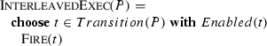
The CoreASM [21] engine implements a generalization of sequentially consistent ASM runs. CoreASM allows one to choose in each step a finite number of agents in A to execute their next step in parallel, instead of choosing only one as ${\textsc {SeqConsExec}}$ does. Thus a run of A is a (finite or infinite) sequence $S_0,S_1,\ldots$ of $\Sigma _A$-states such that

• for the subset $B \subseteq A$ of agents chosen for execution of a step in state $S_0$ the restriction $S_0\downarrow \Sigma _B$ of the state $S_0$ (to the union of the signatures of each element $b \in B$) comprises an initial state for each $b \in B$,

• for each state $S_n$ (except the final one if the sequence is finite) the scheduler component of CoreASM chooses a subset $B \subseteq A$ of agents each of which makes a move in this state such that altogether these moves result in $S_{n+1}$.

To determine subsets $B \subseteq A$ of agents is the role of scheduling. CoreASM allows one to make a non-deterministic choice or to select a maximal set or a set satisfying some priority condition, etc.

2.3.4 Agent’s view of sequentially consistent ASM runs

Witnesses of sequentially consistent ASM runs allow one to reconstruct the original run of each involved agent.

Proposition 1

From each witness of a sequentially consistent ASM run the original sequential run of each agent can be reconstructed.

Proof

Let any witness $S_0,S_1,\ldots$ of a sequentially consistent run of agents $a \in A$ with program asm(a) be given. We reconstruct the original sequential run of a as the a-view $S_0(a),S_1(a),\ldots$ of the witness by induction.

Let $m_0(a),m_1(a),\ldots$ be the sequence of moves a makes in the witness. Let $S_n(a)=S_i\downarrow \Sigma _a$ for the witness state $S_i$ where a makes its move $m_n(a)$. Then $S_i \rightarrow _{m_n(a)} S_{i+1}$ with $S_{i+1}\downarrow \Sigma _a =S_n'(a)$.

Let $S_j$ be the witness state where a makes its next move $m_{n+1}(a)$ (if any) where $i+1 \le j$ (in case a makes no move after $m_n(a)$ the a-view ends with $S_{i+1}\downarrow \Sigma _a$). Let U be such that $S_{i+1}+U=S_j$ (result of the witness segment $S_{i+1},\ldots ,S_j$), so that U is perceived by a as effect of the ‘environment move’ between $m_n(a)$ and $m_{n+1}(a)$. Define $S_{n+1}(a)$ as $S_j \downarrow \Sigma _a$.

2.3.5 Sequentially consistent versus distributed ASM runs

Distributed ASM runs yield sequentially consistent ASM runs for each finite initial run segment.

Proposition 2

For each distributed ASM run $(M,\le )$ and for each finite initial segment  I of $\le$ holds:

Each linearization L of I yields a witness for the sequential consistency of the set of L-subruns of all agents which make a move in L.

Here the L-subrun of agent a denotes the sequence of moves of a in L.

Proof

Let L be any linearization of I—remember that I may be only partially ordered—and A the set of the agents which make some move in L. The L-subruns of the agents in A are well-defined finite executions by the constraint on finite history and the sequentiality of agents in distributed ASM runs. By the coherence condition each single move $m \in L$ is an internal move (as defined in Sect. 2.3) of the agent(m) which executes it. Therefore the moves in L generate a sequence $States(L)=S_0,S_1,\ldots S_k$ of states where each $S_{i+1}$ is the result of applying the i-th move in L to $S_i$ ($0 \le i$) and $S_k=\sigma (I)$.

For each agent a which makes a move in L we can decompose States(L) by its L-subrun $m_0(a),m_1(a),\ldots$ in the form

$$\begin{aligned} S_0 \rightarrow \ldots S_n(a) \rightarrow _{m_n(a)} S_n'(a) \rightarrow \ldots \rightarrow S_{n+1}(a) \ldots \rightarrow S_k \end{aligned}$$

where $S_n(a)$ is the state in States(L) where a makes its n-th move $m_n(a)$ in L ($0\le n$). Therefore, the sequence $M_{n,a}$ of moves other agents make in L after the n-th move $m_n(a)$ of a and before its next move $m_{n+1}(a)$ appears to a after its move $m_n(a)$ and before $m_{n+1}(a)$ as the result of the n-th environment move $m_n(env(a))$. Therefore, States(L) witnesses that the set of L-subruns of all agents which make a move in L is sequentially consistent.

3 Concurrent ASM runs

As explained above, to compute and apply an update set in a state S is considered for single-agent ASMs M as an atomic step forming $S'= S+ \Delta (M,S)$. The success of the ASM method with constructing easy-to-understand models to build and rigorously analyze complex systems in a stepwise manner is to a great extent due to the freedom of abstraction and refinement, which this atomicity concept provides for the modeler, in two respects:

• ground model concern [17] to choose the degree of atomicity of basic update actions such that they directly reflect the level of abstraction of the system to be modeled,

• correct refinement concern [16] to refine this atomicity controllably by hierarchies of more detailed models with finer grained atomic actions, leading from ground models to executable code.

To preserve this freedom of abstraction also for modeling concurrent processes we try to retain as much as possible the atomicity of steps of single process agents. But due to the presence of other agents each agent may have to interact with asynchronously, one must break the synchrony assumption. It turns out that it suffices to split reading and writing of input/output and shared locations as follows: we allow each process to perform in a concurrent run each of its internal steps at its own pace, assuming only that each internal step starts with an atomic read phase and ends with an atomic write phase. Intuitively this means that

• the reading is viewed as locally recording the current values of the input and the shared locations of the process,

• the writing is viewed as writing back new values for the output and the shared locations of the process so that these values become visible to other processes in the run.

This can be achieved by stipulating that a step started (‘by reading’) in a state $S_j$ of a concurrent run is completed (‘by writing back’) in some later, not necessarily the next state $S_n$ of the concurrent run (i.e. such that $j \le n$, thus permitting $j<n$). In fact, such a constraint implies that when a single process M in a given state reads values from shared or monitored locations, no simultaneous updates of these locations by other processes (possibly overlapping with M’s reading) do influence the values read by M in that state. In this way we satisfy Lamport’s read-cleanness requirement that even when reading and writing of a location are overlapping, the reading provides a clear value, either taken before the writings start or after they are terminated [38, 41].

With treating reading resp. writing as atomic operations we deliberately abstract from possibly overlapping reads/writes as they can occur in relaxed memory models; we view describing such models as a matter of further detailing the atomic view at refined levels of abstraction, essentially requiring to specify the underlying caching mechanisms used to access shared locations. For an example we refer to the ASM defined in [63] for the Location Consistency Memory Model.

These considerations lead us to the following definition of concurrent runs of multi-agent ASMs.

Definition 4

Let $\mathcal {A}$ be a set of pairs (a, asm(a)) of agents $a \in A$ with sequential asm(a), called a multi-agent ASM.

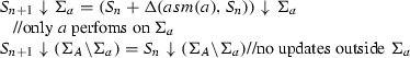
A concurrent run of $\mathcal {A}$ is a sequence $S_0,S_1,\ldots$ of states together with a sequence $A_0,A_1, \ldots$ of subsets of A such that each state $S_{n+1}$ is obtained from $S_n$ by applying to it the updates computed by the agents $a \in A_n$ each of which started its current (internal) step by reading its input and shared locations in some preceding state $S_j$ depending on a. The run terminates in state $S_n$ if the updates computed by the agents in $A_n$ are inconsistent.

The defining condition can be expressed by the following formula where $S_{lastRead(a,n)}$ denotes the state in which a performed its reads of all monitored and shared locations it uses for the current step (so that $lastRead(a,n) \le n$):

$$\begin{aligned} S_{n+1}= S_n + \bigcup _{a \in A_n} \Delta (asm(a),S_{lastRead(a,n)}) \end{aligned}$$

We say that a starts its j-th step in state $S_j$ with $j=lastRead(a,n)$ and completes it in state $S_n$. Remember that $S+U$ is not defined if U is an inconsistent update set.

Remark

The definition generalizes the definition in [20, Def. 2.4.22] of runs of basic ASMs whose moves alternate with environment moves. It relaxes the Single Move Property of sequentially consistent ASM runs since it requires to apply to $S_n$ possibly multiple update sets $\Delta _j$ instead of just one. It trades the read-freshness property for the read-cleanness property by allowing that updates to a location made after an agent read this location may become visible to this agent in the concurrent run only once the agent has completed the step which started with this reading (and thus is based upon it). To determine subsets $A_n$ of agents is the role of scheduling and is the place where message passing algorithms, network communication protocols etc. come in to define particular notions of concurrent system execution.

3.1 Agent’s view of sequentially concurrent ASM runs

For every concurrent ASM run with state sequence $S_0,S_1,\ldots$ and every participating agent a one can define as follows the view of the state sequence by a, namely as sequence

$$\begin{aligned} S_{viewOf(a,0)}, S_{viewOf(a,1)},\ldots \end{aligned}$$

of all states agent a can see in contributing to the run.

Let readMove(n, a) resp. writeMove(n, a) be the number of the state in $S_0,S_1,\ldots$ where a starts resp. completes its n-th step. Then

• $S_{viewOf(a,0)}=S_{readMove(a,0)} \downarrow \Sigma _{asm(a)}$ is an initial state of a,

• $S_{viewOf(a,n+1)}=S_{writeMove(n,a)+k} \downarrow \Sigma _{asm(a)}$ for some $k>0$ such that

  $$\begin{aligned} readMove(n+1,a)=writeMove(n,a)+k \end{aligned}$$

k serves to determine the state where a decides to do its next $readMove(n+1,a)$. Thus a dos not see any state strictly between $S_{viewOf(a,n)}$ and $S_{viewOf(a,n+k)}$ and nothing of any concurrent state that does not belong to its local signature $\Sigma _{asm(a)}$.

3.2 Remark on atomicity of reads/writes

Some authors (see for example [53]) claim that states like the ones we use to define concurrent runs cannot exist. However, epistemologically there is a difference between ‘existence’ and ‘observability’. In a discrete system view one ‘observes’ (‘freezes’) the system at certain moments in time such that each (atomic) location holds a well-defined value, therefore such states have to be assumed to be observable. This is what our definition expresses in terms of local state views, without need to refer to global states.

It is also often argued (e.g. in [53]) that it is unrealistic to assume the reading of a location by one agent in a concurrent run never to interfere with the writing of the same location by another agent. However, to reach the generality needed for a concurrent ASM thesis it seem to be crucial that

• no specific assumption is made on the granularity of the read/write operations,

• the capability of ASMs to capture algorithmic computations at any level of abstraction is preserved.

As for the granularity, with our semantics of concurrent ASM runs one can describe concurrent algorithms also at low abstraction levels with fine-grained access to shared locations under an appropriate concurrency control. An example could be to model atom-by-atom copy mechanisms to a) bring the content of shared locations to private ones, to b) continue the computation by exclusively using the private locations, and to c) complete the step by copying back new values to the shared locations. With our definition we try to guarantee for concurrent algorithms the possibility to faithfully capture the behavioral effect of abstract, complex, concurrently executed steps, in analogy to what has been achieved for sequentially executed steps of sequential algorithms, leaving it to provably correct refinements to realise such steps (typically by computation segments) at lower levels of abstraction (using in the ASM refinement method [16] so-called (1, m)-refinements, for some segment length m). ‘At the heart of the atomicity question is some notion of refinement.’ [4], pg. 37, [5]]

Assuming that the reads and writes a process performs in a step on shared locations are executed atomically reflects an abstract interpretation of the intuitive ‘interaction’ concept in the Concurrency Postulate. One reviewer suggests to consider a more general interaction notion where agents which simultaneously bring in different updates for a location are allowed to negotiate the resulting values for such locations. We think that such cases are captured by Definition 4: the negotiation can be specified by a separate negotiator ASM which steps in when multiple agents present inconsistent location updates. Note also that in [12, 13] (and earlier papers cited there) some specific classes of ASMs with interprocess communication facilities have been studied which lead to a thesis for corresponding classes of algorithms, but the considered runs are not truly concurrent.

3.3 Remark on interleaving

Definition 4 generalizes Lamport’s sequential consistency concept because concurrent ASM runs abstract from strict interleavings of single process executions. Obviously any parallel (simultaneous) updates by several processes can be replaced by an interleaving of these updates that is performed in any order with no process initiating a new step in between; this typical sequential implementation of synchronous parallelism is easily made precise and proved to be correct using the ASM refinement framework [16]. The reason why we prefer to consider in Definition 4 compact runs where synchronous parallelism in single steps allows us to avoid interleaving, is the following: the analysis of compact runs, due to the abstraction from semantically not needed sequentiality, is a) often simpler than the direct analysis of corresponding interleaved runs and b) easily completed (where needed) by a standard refinement argument to a finer-grained analysis of interleaved runs. This is a general experience reflected in the ASM literature, that the abstraction from semantically not needed sequentiality often simplifies both the design and the analysis of complex systems M by first working with an abstract, compact ASM model $M'$ and then refining this (usually by a series of small steps) to the more detailed M. To mention at least one out of many non-trivial examples we point to the analysis of Java and its implementation by the JVM in [62].

4 The Concurrent ASM thesis

As for the sequential ASM thesis proved by Gurevich [29], for the concurrent ASM counterpart we have to prove two statements:

Theorem 1

Plausibility. Each concurrent ASM satisfies the Concurrency Postulate from Sect. 1.

Characterization. Each concurrent process $\mathcal {A} = \{ (a,alg(a)) \mid a \in A \}$ as stipulated by the Concurrency Postulate in Sect. 1 can be simulated by a concurrent ASM $\mathcal {M} = \{ (a,M_a) \mid a \in A \}$ the such that sets of agents and their steps in concurrent runs are in a one-to-one relation (also called lock-step simulation).

The first statement follows from the above described ASM interpretation of the intuitive notions of interaction, single step and state in the Concurrency Postulate and from the definition of concurrent ASM runs because sequential ASMs are a specific way to describe algorithms for sequential processes.

Therefore it suffices to prove the characterization theorem. Since the process components of a concurrent process are sequential, Gurevich’s postulates [29] for sequential algorithms apply to them. We quote those postulates from [20, Ch. 7.2.1]:

• Sequential Time Postulate. Each algorithm $A=alg(a)$ is associated with

  • a set $\mathcal {S}(A)$, the set of states of A,

  • a subset $\mathcal {I}(A)\subseteq \mathcal {S}(A)$, the set of initial states of A,

  • a map $\tau _A:\mathcal {S}(A)\rightarrow \mathcal {S}(A)$, the one-step transformation of A.

• Abstract State Postulate. For each algorithm $A=alg(a)$ holds:

  • the states of A are algebraic first-order structures,

  • all states of A have the same finite signature $\Sigma _A$,

  • the one-step transformation $\tau _A$ does not change the base set of the state,

  • $\mathcal {S}(A)$ and $\mathcal {I}(A)$ are closed under isomorphisms,

  • If $S,S'\in \mathcal {S}(A)$ and $\alpha$ is an isomorphism from S to $S'$, then $\alpha$ is also an isomorphism from $\tau _A(S)$ to $\tau _A(S')$.

• Uniformly Bounded Exploration Postulate. There exists a finite set T—called bounded exploration witness—of ground terms (i.e. without free variables) of A such that the next computation step of the algorithm depends only on that part of the state which can be accessed via terms in T. In other words, whenever two states S and $S'$ coincide over T, then $\Delta (A,S)=\Delta (A,S')$.

Here we use the $\Delta$ notation with the same meaning for ASMs and algorithms.

Therefore we have to construct the rules for sequential ASMs $M_a$ for each agent $a \in A$. The signature for $M_a$, the states and initial states, the one-step transformation function $\tau _a$, etc. are given by Gurevich’s postulates.

4.1 Observation

The construction of the rule for the sequential ASM in the proof of the sequential ASM thesis in [29] does not depend on the entire run $S_0, S_1, \dots$, but only on the state pairs $(S_i,S_{i+1})$, i.e. $(S, \tau (S))$.

We exploit this observation for the concurrent runs defined by $\mathcal {A}$.

So, let $S_0, S_1, \dots$ be the state sequence and $Ag_0, Ag_1, \dots$ the sequence of sets of agents of any concurrent $\mathcal {A}$-run. Consider any state $S_{i+1}$ in this run. Then (by the Concurrency Postulate) we have for some index $lastRead(a,i) \le i$ for each $a \in Ag_i$:

That is, the update set defining the change from state $S_i$ to its successor state $S_{i+1}$ in the concurrent run is a finite union of update sets $\Delta (alg(a_j),S_{i_j} \downarrow \Sigma _{alg(a_j)})$ where $i_j=lastRead(a,i)$. For each agent $a_j \in Ag_i$ participating with a non-empty update set there exists a well-defined previous state $S_{i_j}$ whose (possibly including monitored and shared) location values $alg(a_j)$ determine its update set. The restriction of this state to the signature $\Sigma _j$ of $alg(a_j)$ is a valid state for the sequential algorithm $alg(a_j)$, and the determined update set is the unique update set defining the transition from this state $S_{i_j} \downarrow \Sigma _j$ to its next state via $\tau _a$ (see Lemma 5.1 in [29, p.89]).

Let $R_a$ be the set of all pairs $(S_a,\Delta (S_a))$ of states with their computed update sets where a makes a move in a concurrent $\mathcal {A}$-run, i.e. such that

• $S_a$ is a state of alg(a) and $\Delta (S_a)$ is the unique, consistent update set computed by alg(a) for the transition from $S_a$ to $\tau _a(S_a)$,

• $S_a = S_{i_j} \downarrow \Sigma _{alg(a)}$ for some state $S_{i_j}$ in some non-terminated run of $\mathcal {A}$, in which alg(a) computes an update set that contributes to the definition of a later state in the same run.

We will show the following lemma:

Lemma 1

For each agent $a \in A$ there exists an ASM rule $r_a$ such that for all $(S_a,\Delta (S_a)) \in R_a$ we get $\Delta (S_a)=\Delta (r_a,S_a)$, i.e. the updates the rule $r_a$ yields in state $S_a$ are exactly the updates in $\Delta (S_a)$ determined by alg(a).

The proof of Lemma 1 is given in “Appendix 1”. If we define $r_a$ to be the rule of the sequential ASM $M_a$, we immediately obtain

So any given concurrent $\mathcal {A}$-run $S_0, S_1, \dots$ together with $Ag_0, Ag_1, \dots$ is indeed a concurrent $\mathcal {M}$-run of the concurrent ASM $\mathcal {M} = \{ (a,M_a) \mid a \in A \}$. This proves Theorem 1.

Remark

Note that Theorem 1 remains valid if one of the agents $a \in A$ is not given by an algorithm but as environment. The environment may behave in a non-deterministic way. Though it may participate in the transition from state $S_n$ to $S_{n+1}$ by means of an update set $\Delta$, this set may not depend on any previous state or the dependence may not be functional, e.g. in the case of providing sensor values. In such cases there is no point to look for an ASM to describe the environment.

5 Conclusion

We proposed a semantics for concurrent ASMs by concurrent ASM runs, which overcomes the problems related to Gurevich’s definition of distributed ASM runs. Our definition preserves the characteristic property of ASMs to compute update sets in some state and to apply them to determine a new state. The main difference to sequential ASMs is that the new state is some next state, but not necessarily the next one in the concurrent run, and furthermore that the new state may be the result of finitely many agents bringing in each one its update set computed in some earlier state (depending on the agent). For reasons of simplicity of exposition we restricted our attention to sequential ASMs. However, exploiting further the observation stated in Sect. 4 our definition and the sequential as well as the concurrent ASM thesis work also with basic ASMs (whose moves alternate with environment moves [20, Def. 2.4.22]) and with parallel ASMs (see [7, 11]) for which a conjecture of the second author in [59]—namely that for alg(a) to capture unbounded parallelism, only the bounded exploration witness T has to be changed to a finite set of list comprehension terms—could recently be proven and is available in [22] leading to a parallel ASM thesis).

It seems that the concepts of concurrent runs in other well-known approaches to concurrency we know about satisfy the Concurrency Postulate and can be expressed by concurrent ASM runs, thus experimentally confirming the Concurrent ASM Thesis. A detailed comparative analysis must be left to future work. In the Appendix we sketch however the comparison of concurrent ASMs with two outstanding examples, namely Lamport’s space-time view of distributed systems (“Appendix 2”) and Petri nets (“Appendix 3”). We would appreciate if readers who have reasons to disagree with our expectation let us know their arguments.

Appendices

Appendix 1: Proof of Lemma 1

For the proof of Lemma 1 we strengthen the reasoning in the proof of the sequential ASM-thesis in [29] by exploiting that the correspondence between the updates of the given algorithm and those of the to-be-provided ASM rule holds for every state, including those which in an isolated sequential run of agent a are unreachable but may become reachable when a runs together with other agents. The proof in [29] did not need to consider this case, given that only sequential one-agent runs had to be considered.

Let $a \in A$ be an agent and let T denote a bounded exploration witness of alg(a). We can assume without loss of generality that T is closed under subterms. We call each term $t \in T$ a critical term. If S is a state of alg(a), then let $CV = \{ val_S(t) \mid t \in T \}$ be the set of critical values in state S.

Lemma 2

Let $(f(a_1,\ldots ,a_n),a_0)\in \Delta (S)$ be an update of alg(a) in state S. Then each $a_i$ ($i=0,\dots ,n$) is a critical value in S.

Proof

We adapt the reasoning of Lemma 6.2 in [29, p. 91]. The proof is indirect. Assume $a_i \notin CV$. Create a new structure $S^\prime$ by swapping $a_i$ with a fresh value b not appearing in S, so $S^\prime$ is a state of alg(a). As $a_i$ is not critical, we must have $val_S(t) = val_{S^\prime }(t)$ for all $t \in T$. According to the bounded exploration postulate we obtain $\Delta (S) = \Delta (S^\prime )$ for the update sets produced by alg(a) in states S and $S^\prime$. This gives $(f(a_1,\ldots ,a_n),a_0) \in \Delta (S^\prime )$ contradicting the fact that $a_i$ does not occur in $S^\prime$ and thus cannot occur in the update set created in this state. $\square$

The immediate consequence of Lemma 2 is that there exists an ASM rule $r_S$ such that $\Delta (r_S,S) = \Delta (S)$ holds. Furthermore, $r_S$ only involves critical terms in T. Obviously, the update $(f(a_1,\dots ,a_n),a_0) \in \Delta (S)$ is yielded by a rule $f(t_1,\dots ,t_n) := t_0$ with $t_i \in T$ and $val_S(t_i) = a_i$. So, for each update $u \in \Delta (S)$ we obtain such a rule $r_u$ (but alltogether only finitely many given the finiteness of T), so $r_S = \mathbf {par}\; r_{u_1} \dots r_{u_\ell } \;\mathbf {endpar}$ for $\Delta (S) = \{ u_1,\dots ,u_\ell \}$.

The following lemma states that this result for $r_S$ does not only apply to the single state S.

Lemma 3

The following properties hold for the rule $r_S$:

• If $S^\prime$ is a state, such that S and $S^\prime$ coincide on T, then $\Delta (r_S,S^\prime ) = \Delta (S^\prime )$.

• If $S_1, S_2$ are isomorphic states such that $\Delta (r_S,S_1) = \Delta (S_1)$ holds, then also $\Delta (r_S,S_2) = \Delta (S_2)$ holds.$\square$

These properties are proven in Lemmata 6.7 and 6.8 in [29, p. 93]—we do not repeat the easy proofs here.

The crucial step in the proof of the sequential ASM thesis (and also here) involves the notion of T-similarity [29, p. 93].

Definition 5

Each state S defines an equivalence relation $\sim _S$ on T: $t_1 \sim _S t_2 \Leftrightarrow val_{S}(t_1) = val_S(t_2)$. We call states $S_1, S_2$ T-similar iff $\sim _{S_1} =\, \sim _{S_2}$ holds.

Lemma 4

If state $S^\prime$ is T-similar to S, then $\Delta (r_S,S^\prime ) = \Delta (S^\prime )$ holds.

Proof

We adapt the proof of Lemma 6.9 in [29, p. 93]. Consider a state $S^{\prime \prime }$ isomorphic to $S^\prime$, in which each value that appears also in S is replaced by a fresh one. $S^{\prime \prime }$ is disjoint from S and by construction T-similar to $S^\prime$, hence also T-similar to S.

Thus, according to the second statement in Lemma 3 without loss of generality we can assume that S and $S^\prime$ are disjoint. Define a structure $S^*$ isomorphic to $S^\prime$ by replacing $val_{S^\prime }(t)$ by $val_S(t)$ for all $t \in T$. As S and $S^\prime$ are T-similar, $val_S(t_1) = val_S(t_2) \Leftrightarrow val_{S^\prime }(t_1) = val_{S^\prime }(t_2)$ holds for all critical terms $t_1, t_2$, so the definition of $S^*$ is consistent. Now S and $S^*$ coincide on T, so by the first statement of Lemma 3 we obtain the desired result. $\square$

Now we can complete the proof of Lemma 1. As T is finite, there are only finitely many partitions of T and hence only finitely many T-similarity classes $[S_i]_T$ ($i=0,\dots ,k$). For each such class define a formula $\varphi _i$ such that $val_S(\varphi _i) = true \Leftrightarrow S \in [S_i]_T$ holds. Then define the rule ra as follows:

par IF $\varphi _1$ THEN $r_{S_1}$ ENDIF ...IF $\varphi _k$ THEN $r_{S_k}$ ENDIF endpar

Due to Lemma 4 we have $\Delta (r_a,S) = \Delta (S)$ for all T-similar states S, which completes our proof of Lemma 1.

Appendix 2: Lamport’s space-time view of distributed systems

The space-time view of distributed systems Lamport defined in [39] provides information one can derive from local observations of the runs of the sequential processes which compose a distributed system. This corresponds to the local view of single agents which constitute a concurrent ASM. The partitioning of the systems’ actions by time slicing [61, Ch. 8.3] allows one to define a sequence of global states in the space-time view which illustrates the states in concurrent ASM runs as defined in Sect. 3. In [39] Lamport exemplifies his definitions by equipping each independent process component with a Mutual Exclusion protocol. We show that the resulting distributed system LME can be viewed in a natural way as a concurrent ASM.

Each of the component processes $P_i$ of LME is equipped with its own program (read: a sequential ASM) plus with rules of the Mutual Exlusion protocol (which too can easily be formulated as sequential ASM rules). In each run of LME one can observe for each $P_i$ a sequence of interaction states $S_{i,j}$ resulting from the jth interaction step of $P_i$ in the run—either to Send or to Receive a message—where $S_{i,0}$ is an initial state of $P_i$. By definition the $P_i$-computation segment $]S_{i,j},\ldots , S_{i,j+1}[$ resulting from $P_i$-steps after the jth and before the $j+1$th interaction step is obtained by only internal (non-interaction) steps of $P_i$. Therefore we can view the segment

$$\begin{aligned} ]S_{i,j},\ldots ,S_{i,j+1}] \end{aligned}$$

(excluding $S_{i,j}$ and including $S_{i,j+1}$) as result of one atomic step of say $P_i'$ which leads from $S_{i,j}$ to $S_{i,j+1}$; formally $P_i'$ can be defined as the iteration of $P_i$ until the next interaction step included (what is called a turbo ASM in [20, Ch. 4.1]). One reviewer pointed out that proving the soundness of this abstraction step is related to the method proposed in [43].

This view allows us to define the sequence of concurrent states resulting from the nth interaction step of the component processes $P_i$ as follows:

In $S_n$ each process $P_i$ starts its next local computation segment by reading the data it received from other component processes; when eventually $P_i$ Sends or Receives a message to/from another component process, it gets involved in the next interaction round which yields $S_{n+1}$. Two remarks have to be made here.

• The update sets $\Delta (P_i',S_{i,n})$ are sets of what in the ASM framework are called partial updates (see below), here with respect to the communication medium. In fact multiple processes may simultaneously Send a message to a receiver (e.g. by inserting it into its mailbox) and the receiver may simultaneously Receive such a message (e.g. by deleting it from the mailbox and recording it locally). Thus partial updates handle in particular what Lamport called ‘a notational nuisance’ [39, pg. 561] that is related to the constraint that Sending a message happens before Receiving it. There are no other potentially conflicting updates given that the only shared location in this example is the communication medium.

• The definition of the sequence $(S_n)_n$ exploits that Lamport’s protocol ‘requires the active participation of all the processes’ [39, pg. 562] and corresponds to Fig. 2 in op.cit. where the clock line n connects the nth interaction steps of all processes $P_i$. Other views are possible to form concurrent runs, for example to consider in state $S_n$ only those processes whose next interaction step happens not later than within a given time interval, or before a specific action, or to consider only singleton sets of one interaction step by one agent, etc.

A similar analysis can be made for the notion of distributed business processes in the Subject-Oriented Business Process Modeling framework [18, 23] where one finds an analogous separation of internal and communication steps of interacting agents (called there subjects).

Appendix 3: Petri net runs are special ASM runs

As analyzed already in [20, pg. 297] Petri nets are a specific class of multi-agent ASMs with a particular notion of state and various concepts of run (also called behavior). In fact each Petri net P can be defined as a multi-agent ASM where each agent has exactly one transition t of P as its rule, say P(t); the agent checks whether its transition is Enabled and in case may decide to ${\textsc {Fire}}$ it (or do nothing, a ${\textsc {Skip}}$ move we disregard here to simplify the exposition). Thus the rule P(t) is a sequential ASM of form

The usual understanding one finds in the literature for the state of a traditional Petri net is that of a marking of all its places by tokens, whether ordinary or coloured ones [6, 37, 50].¹ Thus ${\textsc {Fire}}(t)$ yields a set of updates of the locations (marking, p) for the pre/post-places p of t; in the ASM framework locations are defined as pairs (f, a) of a function name and an argument, updates as pairs (loc, val) of locations and values. If Enabled(t), ${\textsc {Fire}}(t)$ yields updates of the form

$$\begin{aligned} ((marking,p),newVal_t(marking(p))). \end{aligned}$$

They are used for writing new values to marking(p) via assignments

$$\begin{aligned} marking(p):=newVal_t(marking(p)) \end{aligned}$$

where the function $newVal_t$ describes how t, if fired alone, at its pre/postplaces adds and/or deletes tokens or (in the case of coloured tokens) changes token values; see the explanation below that this cumulative effect described by $newVal_t$ is an instance of multiple partial updates to structured data. Mutatis mutandis this holds also for the generalization of Petri nets to predicate/transition nets where transitions modify not only a marking function but the characteristic functions $\xi _Q$ of predicates Q that are associated to places [24].

For Petri nets the most commonly used concepts of run (among others) are the following three:

• Petri net runs where each move is the application of a single transition ${\textsc {Fire}}(t)$. They describe the standard interleaving semantics of Petri nets. Such runs are linear orders of executions of single Transitions of a Petri net P, i.e. internal runs of the following sequential ASM:

  

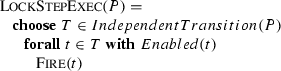
• Petri net runs where each move consists in the simultaneous application of possibly multiple but independently fireable (conflict-free) transitions. They describe the lockstep behavior of Petri nets. Such runs are linear orders of groups of simultaneously executable independent transitions of P, i.e. internal runs of the following basic ASM (where synchronous parallelism is the default case and includes also the use of the universal quantifier $\mathrel {\mathbf {forall}}$). Let IndependentTransition(P) be the set of all sets of conflict-free P-transitions, to be dynamically computed in every state of P; in the ASM framework such locations are called derived locations. One could require IndependentTransition(P) to contain only maximal sets.

  

• Petri net partial order (also called distributed) runs where moves (transition occurrences) are partially ordered by what is called their ‘causal dependency’ (read: token-flow order, a special form of sequential control flow characteristic for Petri nets). For such runs moves that are not ordered by token flow represent transitions that are called to ‘occur concurrently’ to stress that their execution is not forced to be simultaneous (in lock-step) but may happen in any order (including overlapping executions).

  Such runs represent a special case of families of concurrent ASM runs. In fact, when an agent a fires its Petri net transition t the underlying read and write operations a performs to execute t are not only atomic, but happen both in one and the same state in which a starts and completes this step; this is the special case $S_j=S_n$ in Definition 4.

If in a distributed Petri net run conflicts among different enabled transitions occur, due to shared to-be-consumed resources, they yield what in the ASM framework are called inconsistent (whether total or partial) updates.

For an example of inconsistent total updates consider the ${\textsc {MutualExclusion}}$ program in Sect. 2.1: if in a state where $owner(resource)=none$ two different agents $a,a'$ try to simultaneously execute the ${\textsc {Grab}}$ rule, that would yield the update set

$$\begin{aligned} \{((ownerR,resource),a),((owner,resource),a')\}. \end{aligned}$$

This update set represents the attempt to atomically write to owner(resource) the two different values a and $a'$, which is impossible so that the update set cannot be applied and is declared as inconsistent.

Given that a preplace p of a Petri net transition can also be a postplace of the same or another transition, this or these transitions may at the same time remove and insert tokens at p. As a consequence such updates are what in the ASM framework are called cumulative updates, a special vector addition [54] kind of partial updates [32, 56] with their characteristic notion of inconsistency (conflict). Simultaneous removal of m resp. $m'$ and insertion of n resp. $n'$ tokens at place p by agents with two Enabled transitions t resp. $t'$ corresponds to the set

of partial updates to the same location (marking, p); their cumulative effect required by the semantics of Petri nets results in the atomic write operation

$$\begin{aligned} marking(p):=marking(p)-(m + m') + (n+n'). \end{aligned}$$

It is declared by the semantics of Petri nets to be inconsistent if $marking(p) < m+m'$. In fact it has been known for almost half a century that traditional Petri nets are semantically equivalent to factor replacement systems (see [14, pg. 40]) and their geometrical interpretation as vector addition systems, which were introduced by Karp and Miller [54] for the study of decision problems of parallel program schemata, not for the purpose of modeling concurrent systems that come with complex interactions via structured data.

In the literature the intended use of Petri net transitions is suggested by speaking about access/consumption conflicts instead of read/write conflicts. However this does not change the mathematical nature of such shared memory location conflicts. Mathematically speaking the shared locations of (the agent which executes) P(t)—where read/write conflicts with other transitions $P(t')$ may occur—are the following ones: (a) all preplaces of t which are also preplace or postplace of some other transition $P(t')$ of P and (b) all postplaces of t which are also preplace or postplace of some other transition $P(t')$ of P.

References

Abrial, J.R.: The B-Book. Cambridge University Press, Cambridge (1996)
Abrial, J.R.: Modeling in Event-B. Cambridge University Press, Cambridge (2010)
Agha, G.: A Model of Concurrent Computation in Distributed Systems. MIT Press, Cambridge (1986)
Banach, R., Hall, A., Stepney, S.: Retrenchment and the atomicity pattern. In: Fifth IEEE International Conference on Software Engineering and Formal Methods, pp. 37–46 (2007)
Banach, R., Jeske, C., Hall, A., Stepney, S.: Atomicity failure and the retrenchment atomicity pattern. Form. Asp. Comput. 25, 439–464 (2013)
Best, E.: Semantics of Sequential and Parallel Programs. Prentice Hall, Englewood Cliffs (1996)
Blass, A., Gurevich, Y.: Abstract state machines capture parallel algorithms. ACM Trans. Comput. Log. 4(4), 578–651 (2003)
Blass, A., Gurevich, Y.: Ordinary interactive small-step algorithms I. ACM Trans. Comput. Log. 7(2), 363–419 (2006)
Blass, A., Gurevich, Y.: Ordinary interactive small-step algorithms II. ACM Trans. Comput. Log. 8(3), 1–41 (2007)
Blass, A., Gurevich, Y.: Ordinary interactive small-step algorithms III. ACM Trans. Comput. Log. 8(3), 1–51 (2007)
Blass, A., Gurevich, Y.: Abstract state machines capture parallel algorithms: correction and extension. ACM Trans. Comput. Log. 9(3), 1–32 (2008)
Blass, A., Gurevich, Y., Rosenzweig, D., Rossman, B.: Interactive small-step algorithms I: axiomatization. Log. Methods Comput. Sci. 3(4:3), 1–29 (2007)
Blass, A., Gurevich, Y., Rosenzweig, D., Rossman, B.: Interactive small-step algorithms II: abstract state machines and the characterization theorem. Log. Methods Comput. Sci. 3(4:4), 1–35 (2007)
Börger, E.: Computability, complexity, logic (English translation of Berechenbarkeit, Komplexität, Logik, Vieweg-Verlag 1985), Studies in Logic and the Foundations of Mathematics, vol. 128. North-Holland (1989)
Börger, E.: The origins and the development of the ASM method for high-level system design and analysis. J. Univers. Comput. Sci. 8(1), 2–74 (2002)
Börger, E.: The ASM refinement method. Form. Asp. Comput. 15, 237–257 (2003)
Börger, E.: Construction and analysis of ground models and their refinements as a foundation for validating computer based systems. Form. Asp. Comput. 19, 225–241 (2007)
Börger, E., Fleischmann, A.: Abstract state machine nets. Closing the gap between business process models and their implementation. In: Proceedings of the S-BPM ONE 2015. ACM Digital Library. ACM. ISBN:978-1-4503-3312-2 (2015)
Börger, E., Schewe, K.D.: Specifying transaction control to serialize concurrent program executions. In: Ait-Ameur, Y., Schewe, K.D. (eds.) Proceedings ABZ 2014, LNCS. Springer (2014)
Börger, E., Stärk, R.F.: Abstract State Machines: A Method for High-Level System Design and Analysis. Springer, Berlin (2003)
Farahbod, R., et al.: The CoreASM Project. http://www.coreasm.org and http://www.github.com/coreasm
Ferrarotti, F., Schewe, K.D., Tec, L., Wang, Q.: A new thesis concerning synchronised parallel computing—simplified parallel ASM thesis. CoRR abs/1504.06203 (2015).arXiv:1504.06203. Submitted for publication
Fleischmann, A., Schmidt, W., Stary, C., Obermeier, S., Börger, E.: Subject-Oriented Business Process Management. Springer Open Access Book, Heidelberg (2012). www.springer.com/978-3-642-32391-1
Genrich, H.J., Lautenbach, K.: System modelling with high-level Petri nets. Theor. Comput. Sci. 13, 109–136 (1981)
Grädel, E., Nowack, A.: Quantum computing and abstract state machines. In: Börger, E., Gargantini, A., Riccobene, E. (eds.) Abstract State Machines 2003—Advances in Theory and Applications, Lecture Notes in Computer Science, vol. 2589, pp. 309–323. Springer, Berlin (2003)
Gurevich, Y.: Reconsidering Turing’s thesis: toward more realistic semantics of programs. Technical Report CRL-TR-36-84, EECS Department, University of Michigan (1984)
Gurevich, Y.: A new thesis. Amer. Math. Soc. 6(4), 317 (1985)
Gurevich, Y.: Evolving algebras 1993: Lipari guide. In: Börger, E. (ed.) Specification and Validation Methods, pp. 9–36. Oxford University Press (1995)
Gurevich, Y.: Sequential abstract state machines capture sequential algorithms. ACM Trans. Comput. Log. 1(1), 77–111 (2000)
Gurevich, Y., Mani, R.: Group membership protocol: specification and verification. In: Börger, E. (ed.) Specification and Validation Methods, pp. 295–328. Oxford University Press, Oxford (1995)
Gurevich, Y., Rosenzweig, D.: Partially ordered runs: a case study. In: Gurevich, Y., Kutter, P., Odersky, M., Thiele, L. (eds.) Abstract State Machines: Theory and Applications, LNCS, vol. 1912, pp. 131–150. Springer, Berlin (2000)
Gurevich, Y., Tillmann, N.: Partial updates. Theor. Comput. Sci. 336(2–3), 311–342 (2005)
Hamburg, U.: The Petri nets bibliography. http://www.informatik.uni-hamburg.de/TGI/pnbib/index.html
Harris, T., Larus, J., Rajwar, R.: Transactional Memory, 2nd edn. Morgan and Claypool, Los Altos (2010)
Hewitt, C.: What is computation? Actor model versus Turing’s model. In: Zenil, H. (ed.) A Computable Universe: Understanding Computation and Exploring Nature as Computation. Dedicated to the memory of Alan M. Turing on the 100th anniversary of his birth. World Scientific Publishing (2012)
Hoare, C.A.R.: Communicating Sequential Processes. Prentice-Hall, Englewood Cliffs (1985)
Jensen, K.: Coloured Petri Nets - Basic Concepts, Analysis Methods and Practical. Monographs in Theoretical Computer Science. An EATCS Series vol. 3. Springer, Berlin (1997). doi:10.1007/978-3-642-60794-3
Lamport, L.: A new solution of Dijkstra’s concurrent programming problem. Commun. ACM 17(8), 453–455 (1974)
Lamport, L.: Time, clocks, and the ordering of events in a distributed system. Commun. ACM 21(7), 558–565 (1978)
Lamport, L.: How to make a multiprocessor computer that correctly executes multiprocess programs. IEEE Trans. Comput. 28(9), 690–691 (1979)
Lamport, L.: On interprocess communication. Part I: Basic formalism. Part II: algorithms. Distrib. Comput. 1, 77–101 (1986)
Lamport, L.: Specifying Systems: The TLA+ Language and Tools for Hardware and Software Engineers. Addison-Wesley (2003). http://lamport.org
Lamport, L., Schneider, F.B.: Pretending Atomicity. DEC Systems Research Center (1989)
Lamport, L., Lynch, N.: Distributed computing: models and methods. In: J. van Leeuwen (ed.) Handbook of Theoretical Computer Science, pp. 1157–1199. Elsevier (1990)
Lynch, N.: Distributed Algorithms. Morgan Kaufmann (1996). ISBN:978-1-55860-348-6
Mazurkiewicz, A.: Trace Theory, pp. 279–324. Springer, Berlin (1987)
Mazurkiewicz, A.: Introduction to trace theory. In: Diekert, V., Rozenberg, G. (eds.) The Book of Traces, pp. 3–67. World Scientific, Singapore (1995)
Milner, R.: A Calculus of Communicating Systems. Springer (1982). ISBN 0-387-10235-3
Milner, R.: Communicating and Mobile Systems: The Pi-Calculus. Springer (1999). ISBN 9780521658690
Peterson, J.: Petri Net Theory and the Modeling of Systems. Prentice-Hall, Englewood Cliffs (1981)
Petri, C.A.: Kommunikation mit automaten. Ph.D. thesis, Institut für Instrumentelle Mathematik der Universität Bonn (1962). Schriften des IIM Nr. 2
Plosila, J., Sere, K., Walden, M.: Design with asynchronously communicating components. In: de Boer et al., F. (ed.) Proceedings of FMCO 2002, No. 2852 in LNCS, pp. 424–442. Springer (2003)
Prinz, A., Sherratt, E.: Distributed ASM-pitfalls and solutions. In: Aït-Ameur, Y., Schewe, K.D. (eds.) Abstract State Machines, Alloy, B, TLA, VDM and Z—Proceedings of the 4th International Conference (ABZ 2014), LNCS, vol. 8477, pp. 210–215. Springer, Toulouse (2014)
Karp, R.M., Miller, R.: Parallel program schemata. J. Comput. Syst. Sci. 3, 147–195 (1969)
Roscoe, A.: The Theory and Practice of Concurrency. Prentice-Hall, Englewood Cliffs (1997)
Schewe, K.D., Wang, Q.: A customised ASM thesis for database transformations. Acta Cybern. 19(4), 765–805 (2010)
Schewe, K.D., Wang, Q.: XML database transformations. J. Univers. Comput. Sci. 16(20), 3043–3072 (2010)
Schewe, K.D., Wang, Q.: Partial updates in complex-value databases. In: Heimbürger, A., et al. (eds.) Information and Knowledge Bases XXII, Frontiers in Artificial Intelligence and Applications, vol. 225, pp. 37–56. IOS Press, Amsterdam (2011)
Schewe, K.D., Wang, Q.: A simplified parallel ASM thesis. In: Derrick, J., et al. (eds.) Abstract State Machines, Alloy, B, VDM, and Z—Third International Conference (ABZ 2012), LNCS, vol. 7316, pp. 341–344. Springer (2012)
Schewe, K.D., Wang, Q.: Synchronous parallel database transformations. In: Lukasiewicz, T., Sali, A. (eds.) Foundations of Information and Knowledge Bases (FoIKS 2012), LNCS, vol. 7153, pp. 371–384. Springer, Berlin (2012)
Schneider, F., Lamport, L.: Paradigms for distributed programs. In: Distributed Systems, LNCS, vol. 190. Springer (1985)
Stärk, R.F., Schmid, J., Börger, E.: Java and the Java Virtual Machine: Definition, Verification, Validation. Springer, Berlin (2001)
Wallace, C., Tremblay, G., Amaral, J.N.: An abstract state machine specification and verification of the location consistency memory model and cache protocol. J. Univers. Comput. Sci. 7(11), 1089–1113 (2001)
Wang, Q.: Logical Foundations of Database Transformations for Complex-Value Databases.Logos (2010). http://logos-verlag.de/cgi-bin/engbuchmid?isbn=2563&lng=deu&id=
Wegner, P.: Why interaction is more powerful than algorithms. Commun. ACM 40, 80–91 (1997)
Winskel, G., Nielsen, M.: Models for concurrency. In: Abramsky, S., Gabbay, D., Maibaum, T.S.E. (eds.) Handbook of Logic and the Foundations of Computer Science: Semantic Modelling, vol. 4, pp. 1–148. Oxford University Press, Oxford (1995)
Acknowledgments
The first author thanks numerous colleagues with whom he discussed over the years the problems with Gurevich’s distributed ASM runs and what ‘concurrency’ could reasonably mean for ASMs. This includes in particular R. Stärk, D. Rosenzweig, A. Raschke, A. Prinz, M. Lochau, U. Glässer, U. Goltz, A. Fleischmann, I. Durdanović, A. Cisternino, P. Arcaini. We also thank one of the anonymous referees for very careful readings of two previous versions of this paper and for numerous insightful questions and comments for its improvement.
Author information
Authors and Affiliations
Corresponding author
Additional information
The first author gratefully acknowledges support for part of the work by a fellowship from the Alexander von Humboldt Foundation, sequel to the Humboldt Forschungspreis awarded in 2007/2008.
The research reported in this paper results from the project Behavioural Theory and Logics for Distributed Adaptive Systems supported by the Austrian Science Fund (FWF): [P26452-N15]. It was further the supported by the Austrian Research Promotion Agency (FFG) through the COMET funding for the Software Competence Center Hagenberg.