Mass estimation

Abstract

This paper introduces mass estimation—a base modelling mechanism that can be employed to solve various tasks in machine learning. We present the theoretical basis of mass and efficient methods to estimate mass. We show that mass estimation solves problems effectively in tasks such as information retrieval, regression and anomaly detection. The models, which use mass in these three tasks, perform at least as well as and often better than eight state-of-the-art methods in terms of task-specific performance measures. In addition, mass estimation has constant time and space complexities.

1 Introduction

‘Estimation of densities is a universal problem of statistics (knowing the densities one can solve various problems).’ —Vapnik (2000).

Density estimation has been the base modelling mechanism used in many techniques designed for tasks such as classification, clustering, anomaly detection and information retrieval. For example in classification, density estimation is employed to estimate the class-conditional density function (or likelihood function) p(x|j) or posterior probability p(j|x)—the principal function underlying many classification methods; e.g., mixture models, Bayesian networks, Naive Bayes. Examples of density estimation include kernel density estimation, k-nearest neighbours density estimation, maximum likelihood procedures and Bayesian methods.

Ranking data points in a given data set in order to differentiate core points from fringe points in a data cloud is fundamental in many tasks, including anomaly detection and information retrieval. Anomaly detection aims to rank anomalous points higher than normal points; information retrieval aims to rank points similar to a query higher than dissimilar points. Many existing methods (e.g., Bay and Schwabacher 2003; Breunig et al. 2000; Zhang and Zhang 2006) have employed density to provide the ranking; but density estimation is not designed to provide a ranking.

We show in this paper that a new base modelling mechanism called mass estimation possesses different properties from those offered by density estimation:

• A mass distribution stipulates an ordering from core points to fringe points in a data cloud. In addition, this ordering accentuates the fringe points with a concave function derived from data, resulting in fringe points having markedly smaller mass than points close to the core points.

• Mass estimation is more efficient than density estimation because mass is computed by simple counting and it requires only a small sample through an ensemble approach. Density estimation (often used to estimate p(x|j) and p(j|x)) requires a large sample size in order to have a good estimation and is computationally expensive in terms of time and space complexities (Duda et al. 2001).

Mass estimation has two advantages in relation to efficacy and efficiency. First, the concavity property mentioned above ensures that fringe points are ‘stretched’ to be farther from the core points in a mass space—making it easier to separate fringe points from those points close to core points. This property in mass space can then be exploited by a machine learning algorithm to achieve a better result for the intended task than applying the same algorithm in the original space without this property. We show the efficacy of mass in improving the task-specific performance of four existing state-of-the-art algorithms in information retrieval and regression tasks. The significant improvements are achieved through a simple mapping from the original space to a mass space using the mass estimation mechanism introduced in this paper.

Second, mass estimation offers to solve a ranking problem more efficiently using the ordering derived from data directly—without expensive distance (or related) calculations. An example of inefficient application is in anomaly detection tasks where many methods have employed distance or density to provide the required ranking. An existing state-of-the-art density-based anomaly detector LOF (Breunig et al. 2000) (which has quadratic time complexity) completes a job involving half a million data points in more than five hours; yet the mass-based anomaly detector we have introduced here completes it in less than 20 seconds! Section 6.3 provides the details of this example.

The rest of the paper is organised as follows. Section 2 introduces mass and mass estimation, together with their theoretical properties. We also describe methods for one-dimensional mass estimation. We extend one-dimensional mass estimation to multi-dimensional mass estimation in Sect. 3. We provide an implementation of multi-dimensional mass estimation in Sect. 4. Section 5 describes a mass-based formalism which serves as a basis of applying mass to different data mining tasks. We realise the formalism in three different tasks: information retrieval, regression and anomaly detection, and report the empirical evaluation results in Sect. 6. The relations to kernel density estimation, data depth and other related work are described in Sects. 7, 8 and 9, respectively. We provide conclusions and suggest future work in the last section.

2 Mass and mass estimation

Data mass or mass, in its simplest form, is defined as the number of points in a region. Any two groups of data in the same domain have the same mass if they have the same number of points, regardless of the characteristics of the regions they occupy (e.g., density, shape or volume). Mass in a given region is thus defined by a rectangular function which has the same value for the entire region in which the mass is measured.

To estimate the mass for a point and thus the mass distribution of a given data set, a more sophisticated form is required. The intuition is based on the simplest form described above, but multiple (overlapping) regions covering a point are generated. The mass for the point is then derived from an average of masses from all regions covering the point. We show two ways to define these regions. The first is to generate all possible regions through binary splits from the given data points; and the second is to generate random axis-parallel regions within the confine covered by a data sample. The first is described in this section and the second is described in Sect. 3.

Each region can be defined in multiple levels where a higher level region covering a point has a smaller volume than that of a lower level region covering the same point. We show that the mass distribution has special properties: (i) the mass distribution defined by level-1 regions is a concave function which has the maximum mass at the centre of the data cloud, irrespective of its density distribution, including uniform and U-shape distributions; and (ii) higher level regions are required to model multi-modal mass distributions.

Note that mass is not a probability mass function, and it does not provide a probability, as the probability density function does through integration.

In Sect. 2.1, we show (i) how to estimate a mass distribution for a given data set through binary splits and (ii) the theoretical properties of mass estimation. Section 2.2 describes an approximation to the theoretical mass estimation which works more efficiently in practice. The symbols and notations used are provided in Table 1.

Table 1 Symbols and notations

2.1 Mass distribution estimation

In this section, we first show in Sect. 2.1.1 a mass distribution estimation that uses binary splits in the one-dimensional setting, where each binary split separates the one-dimensional space into two non-empty regions. In Sect. 2.1.2, we then generalise the treatment using multiple levels of binary splits.

2.1.1 Mass distribution estimation using binary splits

Here, we employ a binary split to divide the data set into two separate regions and compute the mass in each region. The mass distribution at point x is estimated to be the sum of all ‘weighted’ masses from regions occupied by x, as a result of n−1 binary splits for a data set of size n.

Let x ₁<x ₂<⋯<x _n−1<x _n on the real line,¹ $x_{i} \in\mathcal{R}$ and n>1. Let s _i be the binary split between x _i and x _i+1, yielding two non-empty regions having two masses $m_{i}^{L}$ and $m_{i}^{R}$.

Definition 1

Mass base function: m _i (x) as a result of s _i , is defined as

$$m_i(x)= \left \{ \begin{array}{l@{\quad}l} m_i^L & \mbox{if } x \mbox{ is on the left of } s_i \\ m_i^R & \mbox{if } x \mbox{ is on the right of } s_i\\ \end{array} \right . $$

Note that $m_{i}^{L} = n-m_{i}^{R} = i$.

Definition 2

Mass distribution: mass(x _a ) for a point x _a ∈{x ₁,x ₂,…,x _n−1,x _n } is defined as a summation of a series of mass base functions m _i (x) weighted by p(s _i ) over n−1 splits as follows, where p(s _i ) is the probability of selecting s _i .

(1)

Note that we have defined $\sum_{i=q}^{r} f(i) = 0$, when r<q for any function f.

Example

For an example of five points x ₁<x ₂<x ₃<x ₄<x ₅, Fig. 1 shows the resultant m _i (x) due to each of the four binary splits s ₁,s ₂,s ₃,s ₄; and their associated masses over four splits are given below:

Fig. 1

Examples of mass base function m _i (x) due to each of the four binary splits: s ₁,s ₂,s ₃,s ₄

For a given data set, p(s _i ) can be estimated on the real line as p(s _i )=(x _i+1−x _i )/(x _n −x ₁)>0, as a result of a random selection of splits based on a uniform distribution.²

For a point x∉{x ₁,x ₂,…,x _n−1,x _n }, mass(x) is defined as an interpolation between two masses of adjacent points x _i and x _i+1, where x _i <x<x _i+1.

Theorem 1

mass(x _a ) is maximised at a=n/2 for any density distribution of {x ₁,…,x _n }; and the points x _a , where x ₁<x ₂<⋯<x _n−1<x _n on the real line, can be ordered based on mass as follows.

Proof

The difference in mass between two consecutive points x _a and x _a+1 differs in only one term, i.e., the mass associated with p(s _a ); and ∀i≠a, the terms for p(s _i ) have the same mass.

(2)

Thus,

$$\mathit{sign}\bigl(\mathit{mass}(x_a) - \mathit{mass}(x_{a+1}) \bigr) = \left \{ \begin{array}{l@{\quad}l} \mathrm{negative} & \mbox{if $a < n/2$} \\ 0 & \mbox{if $a = n/2$} \\ \mathit{positive} & \mbox{if $a > n/2$} \end{array} \right . $$

The point x _n/2 can be regarded as the median. Note that the number of points with the maximum mass depends on whether n is odd or even: When n is an odd integer, only one point has the maximum mass at x _median , where median=⌈n/2⌉; when n is an even integer, two points have the maximum mass at a=n/2 and a=1+n/2. □

Theorem 2

mass(x _a ) is a concave function defined w.r.t. {x ₁,x ₂,…,x _n }, when p(s _i )=(x _i+1−x _i )/(x _n −x ₁) for n>2.

Proof

We only need to show that the gradient of x _a is non-increasing, i.e., g(x _a )>g(x _a+1) for each a.

Let g(x _a ) be the gradient between x _a and x _a+1, and from (2):

$$g(x_a) = \frac{\mathit{mass}(x_{a+1})- \mathit{mass}(x_a)}{x_{a+1} - x_a} = \frac{n - 2a}{x_n - x_1} $$

The result follows: g(x _a )>g(x _a+1) for a∈{1,2,…,n−1}. □

Corollary 1

A mass distribution estimated using binary splits stipulates an ordering, based on mass, of the points in a data cloud from x _n/2 (with the maximum mass) to the fringe points (with the minimum mass at either side of x _n/2), irrespective of the density distribution including uniform density distribution.

Corollary 2

The concavity of mass distribution stipulates that fringe points have markedly smaller mass than points close to x _n/2.

The implication from Corollary 2 is that fringe points are ‘stretched’ to be farther away from the median in a mass space than in the original space—making it easier to separate fringe points from those points close to the median. The mass space is mapped from the original space through mass(x). This property in mass space can then be exploited by a machine learning algorithm to achieve a better result for the intended task than applying the same algorithm in the original space without this property. We will show that this simple mapping significantly improves the performance of four existing algorithms in information retrieval and regression tasks in Sects. 6.1 and 6.2.

Equation (1) is sufficient to provide a mass distribution corresponding to a unimodal density function or a uniform density function. To better estimate multi-modal mass distributions, multiple levels of binary splits need to be carried out. This is provided in the following.

2.1.2 Level-h mass distribution estimation

If we treat the mass estimation defined in the last subsection as level-1 estimation, then level-h estimation can be viewed as localised versions of the basic level-1 estimation.

Definition 3

The level-h mass distribution for a point x _a ∈{x ₁,…,x _n }, where h<n, is expressed as

(3)

Here a high level mass distribution is computed recursively by using the mass distributions obtained at lower levels. A binary split s _i in a level-h(>1) mass distribution produces two level-(h-1) mass distributions: (a) $\mathit{mass}_{i}^{L}(x,h\mbox{-}1)$—the mass distribution on the left of split s _i which is defined using {x ₁,…,x _i }; and (b) $\mathit{mass}_{i}^{R}(x,h\mbox{-}1)$—the mass distribution on the right which is defined using {x _i+1,…,x _n }. Equation (1) is the mass distribution at level-1.

Figure 2 shows two (out of 19 splits) required to compute level-2 mass estimation, mass(x,h=2), from a data set of 20 points. Each split produces two level-1 mass estimations: $\mathit{mass}_{i}^{L}(x,h=1)$ and $\mathit{mass}_{i}^{R}(x,h=1)$. Note that level-1 mass distribution is concave, as proven in Theorem 2. This example shows the results of two splits s _i=7 and s _i=11, where each level-1 mass distribution is concave.

Fig. 2

Two examples of $\mathit{mass}_{i}^{L}(x,h=1)$ and $\mathit{mass}_{i}^{R}(x,h=1)$ due to s _i=7 and s _i=11 in the process to get mass(x,h=2) from a data set of 20 points with uniform density distribution. The resultant mass(x,h=2) is shown in Fig. 3(a)

Using the same analysis as in the proof for Theorem 1, the above equation can be re-expressed as:

(4)

As a result, only the mass for the first point x ₁ needs to be computed using (3). Note that it is more efficient to compute the mass distribution from the above equation which has time complexity O(n ^h+1); the computation using (3) has complexity O(n ^h+2).

Definition 4

A level-h mass distribution stipulates an ordering of the points in a data cloud from α-core points to the fringe points. Let α-neighbourhood of a point x be defined as N _α (x)={y∈D|dist(x,y)≤α} for some distance function dist(⋅,⋅). Each α-core point x ^∗ in a data cloud has the highest mass value ∀x∈N _α (x ^∗). A small α defines local core point(s); and a large α, which covers the entire value range for x, defines global core point(s).

Examples of level-h mass estimation in comparison with kernel density estimation are provided in Fig. 3. Note that h=1 mass estimation looks at the data as a group, and it produces a concave function. As a result, an h=1 mass estimation always has its global core point(s) at the median, regardless of the underlying density distribution—see the four examples of h=1 mass estimation in Fig. 3.

Fig. 3

Examples of level-h mass distribution for h=1,2,3 and density distribution from kernel density estimation: Gaussian kernel with bandwidth =0.1 (for the first three figures) and 0.01 (for the last figure in order to show the density spike). The data sets have 20 points each for the first three figures, and the last one has 50 points

For h>1 mass distribution, though there is no guarantee for a concave function any more as a whole, our simulation shows that each cluster within the data cloud (if they exist) exhibits a concave function and it becomes more distinct (as a concave function) as h increases. An example is shown in Fig. 3(b) which has a trimodal density distribution. Notice that the h>1 mass distributions have three α-core points for some α, e.g., 0.2. Other examples are shown in Figs. 3(c) and 3(d).

Traditionally, one can estimate the core-ness or the fringe-ness of non-uniformly distributed data to some degree by using density or distance (but not in uniform density distribution). Mass allows one to do that in any distribution without density or distance calculation—the key computational expense in all methods that employ them. For example in Fig. 3(c) which has a skew density distribution, the distinction between near fringe points and far fringe points are less obvious using density, unless distances are computed to reveal the difference. In contrast, mass distribution depicts the relative distance from x _median using the fringe points’ mass values, without further calculation.

Figure 3(d) shows an example where there are clustered anomalies which are denser than the normal points (shown in the bigger cluster on the left of the figure). Anomaly detection based on density will identify all these clustered anomalies as more ‘normal’ than the normal points because anomalies are defined as points having low density. In sharp contrast, h=1 mass estimation will correctly rank them as anomalies which have the third lowest mass values. These points are interpreted as points at the fringe of the data cloud of normal points which have higher mass values.

This section has described properties of mass distribution from a theoretical perspective. Though it is possible to estimate mass distribution using (1) and (3), they are limited by its high computational cost. We suggest a practical mass estimation method in the next subsection. We use the term ‘mass estimation’ and ‘mass distribution estimation’ interchangeably hereafter.

2.2 Practical one-dimensional level-h mass estimation

Here we devise an approximation to (3) using random subsamples from a given data set.

Definition 5

$\mathit{mass}(x,h|\mathcal{D})$ is the approximate mass distribution for a point $x \in\mathcal{R}$, defined w.r.t. $\mathcal{D} = \{x_{1},\ldots, x_{\psi}\}$, where $\mathcal{D}$ is a random subset of the given data set D, and ψ≪|D|, h<ψ.

Here we employ a rectangular function to define mass for a region encompassing each point $x \in\mathcal{D}$. $\mathit{mass}(x,h|\mathcal{D})$ is implemented using a lookup table where a region for each point $x_{i} \in\mathcal{D}$ covers a range (x _i−1+x _i )/2≤x<(x _i+1+x _i )/2 and has the same $\mathit{mass}(x_{i},h|\mathcal{D})$ value for the entire region. The range for each of the two end-points is set to have equal length on either side of the point. An example is provided in Fig. 4(a).

Fig. 4

(a) An example of practical mass distribution $\mathit{mass}(x,h|\mathcal{D})$ for 5 points, assuming a rectangular function for each point. (b) Correlation between the orderings provided by mass(x,1) and $\mathit{mass}(x,1|\mathcal{D})$ for two data sets: one-dimensional Gaussian density distribution and the COREL data set used in Sect. 6.1 (whose result is averaged over 67 dimensions)

In addition, a number of mass distributions needs to be constructed from different samples in order to have a good approximation, that is,

$$ \overline{\mathit{mass}}(x,h) \approx\frac{1}{c} \sum_{k=1}^c \mathit{mass}(x,h|\mathcal{D}_k) $$

(5)

The computation of mass(x,h) using the given data set D costs O(|D|^h+1) in terms of time complexity; whereas $\mathit{mass}(x,h|\mathcal {D})$ costs O(ψ ^h+1).

Only relative, not absolute, mass is required to provide an ordering between instances. For h=1, because the relative mass is w.r.t. the median and the median is a robust estimator (Aloupis 2006)—that is why small subsamples produce a good estimator for ordering. While this reason cannot be applied to h>1 (and multi-dimensional mass estimation to be discussed in the next section) because the notion of median is undefined, our empirical results in Sect. 6 show that all these mass estimations using small subsamples produce good results.

In order to show that relative performance of mass(x,1) and $\mathit{mass}(x,1|\mathcal{D})$, we compare the ordering results based on mass values in two separate data sets: the one-dimensional Gaussian density distribution and the COREL data set; each of the data sets has 10000 data points. Figure 4(b) shows the correlation (in terms of Spearman’s rank correlation coefficient) between the orderings provided by mass(x,1) using the entire data set and $\mathit{mass}(x,1|\mathcal{D})$ using ψ=8. They achieve very high correlations when c≥100 for both data sets.

The ability to use a small sample, rather than a large sample, is a key characteristic of mass estimation.

3 Multi-dimensional mass estimation

Ting and Wells (2010) describe a way to generalise the one-dimensional mass estimation we have described in the last section. We reiterate the approach in this section but the implementation we employed (to be described in Sect. 4) differs. Section 9 provides the details of these differences.

The approach proposed by Ting and Wells (2010) eliminates the need to compute the probability of a binary split, p(s _i ); and it gives rise to randomised versions of (1), (3) and (5).

The idea is to generate multiple random regions which cover a point, and then the mass for that point is estimated by averaging all masses from all those regions. We show that random regions can be generated using axis-parallel splits called half-space splits. Each half-space split is performed on a randomly selected attribute in a multi-dimensional feature space. For a h-level split, each half-space split is carried out h times recursively along every path in a tree structure. Each h-level (axis-parallel) split generates 2^h non-overlapping regions. Multiple h-level splits are used to estimate mass for each point in the feature space.

The multi-dimensional mass estimation requires two functions. First, it needs a function that generates random regions covering each point in the feature space. This function is a generalisation of the binary split into half-space splits or 2^h-region splits when h levels of half-space splits are used. Second, a generalised version of the mass base function is used to define mass in a region. The formal definition follows.

Let x be an instance in $\mathcal{R}^{d}$. Let T ^h(x) be one of the 2^h regions in which x falls into; T ^h(⋅) is generated from the given data set D, and $T^{h}(\cdot |\mathcal{D})$ is generated from $\mathcal{D} \subset D$; and m be the number of training instances in the region.

The generalised mass base function: m(T ^h(x)) is defined as

$$\mathbf{m}\bigl(T^h(\mathbf{x})\bigr)= \left \{ \begin{array}{l@{\quad}l} \mathsf{m} & \mbox{if } \mathbf{x} \mbox{ is in a region of $T^{h}$ having $\mathsf{m}$ instances} \\ 0 & \mbox{otherwise}\\ \end{array} \right . $$

In one-dimensional problems, (1), (3) and (5) can now be approximated as follows:

(6)

(7)

(8)

where c>0 is the number of random regions to be used to define the mass for x.

Here every $T_{k}^{h}$ is generated randomly with equal probability. Note that p(s _i ) in (1) has the same assumption.

Since T ^h is defined in multi-dimensional space, the multi-dimensional mass estimation is the same as (8) by simply replacing x with x:

$$ \overline{\mathit{mass}}(\mathbf{x},h) \approx \frac{1}{c} \sum_{k=1}^{c} \mathbf{m} \bigl(T_k^h(\mathbf{x}|\mathcal{D}_k)\bigr) $$

(9)

Like its one-dimensional counterpart, the multi-dimensional mass estimation stipulates an ordering from core points (having high mass) to fringe points (having low mass) in a data cloud, regardless of its density distribution. While we do not have a proof of this property for multi-dimensional mass estimation, empirical results suggest that it is. This property is shown in Fig. 5(a) using h=1, where the highest mass value is at the centre of the entire data cloud, when the four clusters are treated as a single data cloud; while the four clusters are scattered in each of the four quadrants. Mass values become lower as they move away from the centre. Note that though this implementation of multi-dimensional mass estimation does not guarantee concavity, the approximation of the ordering is sufficiently close to a concave function (in regions with data) to produce the required ranking for different purposes (see Sect. 6).

Fig. 5

Contour maps of multi-dimensional mass distribution for a two-dimensional data set with four clusters (each containing 50 points), where points in each cluster are marked with a distinct marker. The points are randomly drawn from Gaussian distributions with unit standard deviation and means located at (2; 2), (−2; 2), (−2; −2) and (2; −2), respectively. The two figures are produced using h=1 and h=32, respectively. Other parameters are set as follows: c=1000 and $\psi= |\mathcal{D}|=64$. The algorithm used to generate these contour maps will be described in Sect. 4.2. The legend indicates the colour-coded mass values

Figure 5(b) shows the contour map for h=32 on the same data set. It demonstrates that multi-dimensional mass estimation can use a high h level to model multi-modal distribution.

We show in Sect. 6 that both $\mathit{mass}(x,h|\mathcal {D})$ and $\mathbf{m}(T^{h}(\mathbf{x}|\mathcal{D}))$ (in (5) and (9), respectively) can be employed effectively for three different tasks: information retrieval, regression and anomaly detection, through the mass-based formalism described in Sect. 5. We shall describe the implementation of multi-dimensional mass estimation in the next section.

4 Half-Space Trees for mass estimation

This section describes the implementation of T ^h using Half-Space Tree. Two variants are provided. We have used the second variant of Half-Space Tree to implement the multi-dimensional mass estimation.

4.1 Half-Space Tree

The motivation of the proposed method, Half-Space Tree, comes from the fact that equal-size regions contain the same mass in a space with uniform mass distribution, regardless of the shapes of the regions. This is shown in Fig. 6(a), where the space enveloped by the data is split into equal-size half-spaces recursively three times into eight regions. Note that the shapes of the regions may be different because the splits at the same level may not use the same attribute.

Fig. 6

Half-space subdivisions of: (a) uniform mass distribution; and (b) non-uniform mass distribution

The binary half-space split ensures that every split produces two equal-size half-spaces, each containing exactly half of the mass before the split under a uniform mass distribution. This characteristic enables us to compute the relationship between any two regions easily. For example, the mass in every region shown in Fig. 6(a) is the same, and it is equivalent to the original mass divided by 2³ because three levels of binary half-space splits have been applied. A deviation from the uniform mass distribution allows us to rank the regions based on mass. Figure 6(b) provides such an example in which a ranking of regions based on mass provides an order of the degrees of anomaly in each region.

Definition 6

Half-Space Tree is a binary tree in which each internal node makes a half-space split into two equal-size regions, and each external node terminates further splits. All nodes record the mass of the training data in their own regions.

Let T ^h[i] be a Half-Space Tree with depth level i; and m(T ^h[i]) or short for m[i] be the mass in one of the regions at level i.

The relationship between any two regions is expressed using mass with reference to m[0] at depth level=0 (the root) of a Half-Space Tree.

Under uniform mass distribution, the mass at level i is related to mass at level 0 as follows:

$$\mathbf{m}[0] = \mathbf{m}[i] \times2^i, $$

or mass values between any two regions at levels i and j, ∀i≠j, are related as follows:

$$\mathbf{m}[i] \times2^i = \mathbf{m}[j] \times2^j. $$

Under non-uniform mass distribution, the following inequality establishes an ordering between any two regions at different levels:

$$\mathbf{m}[i] \times2^i < \mathbf{m}[j] \times2^j. $$

We employ the above property to rank instances and define the (augmented) mass for Half-Space Tree as follows.

$$ s(\mathbf{x}) = \mathbf{m}[ \ell] \times2^\ell, $$

(10)

where ℓ is the depth level of an external node with m[ℓ] instances in which a test instance x falls into.

Mass is estimated using m[ℓ] only if a Half-Space Tree has all external nodes at the same depth level. The estimation is based on augmented mass, m[ℓ]×2^ℓ, if the external nodes have differing depth levels. We describe two such variants of Half-Space Tree below.

HS-Tree: based on mass only. The first variant, HS-Tree, builds a balanced binary tree structure which makes a half-space split at each internal node and all external nodes have the same depth. The number of training instances falling into each external node is recorded and it is used for mass estimation. An example of HS-Tree is shown in Fig. 7(a).

Fig. 7

Half-Space Tree: (a) HS-Tree: An HS-Tree for the data shown in Fig. 6(a) has m _i =4,∀i, which are m[ℓ=3] (i.e., mass at level 3). (b) HS*-Tree: An example of a special case of HS*-Tree when the size limit is set to 1

HS*-Tree: based on augmented mass. Unlike HS-Tree, the second variant, HS*-Tree, whose external nodes have differing depth levels. The mass estimated from HS*-Tree is defined in equation (10) in order to account for different depths. We call this augmented mass because the mass is augmented in the calculation by the depth level in HS*-Tree, as opposed to mass only in HS-Tree.

In a special case of HS*-Tree, the tree growing process at a branch will only terminate to form an external node if the training data size at the branch is 1 (i.e., the size limit is set to 1). Here the mass estimated depends on depth level only, i.e., 2^ℓ or simply ℓ. In other words, the depth level becomes a proxy for mass in HS*-Tree when the size limit is set to 1. An example of HS*-Tree, when the size limit is set to 1, is shown in Fig. 7(b).

Since the two variants have similar performance, we focus on HS*-Tree only in this paper because it builds a smaller-sized tree than HS-Tree which may grow many branches with zero mass—this saves on training time and memory space requirements.

4.2 Algorithm to generate Half-Space Trees

Half-Space Trees estimate a mass distribution efficiently, without density or distance calculations or clustering. We first describe the training procedure, then the testing procedure, and finally the time and space complexities.

Training. The procedure to generate a Half-Space Tree is shown in Algorithm 1. It starts by defining a (random) range for each dimension in order to form a work space which covers all the training data. The InitialiseWorkSpace(⋅) function in Algorithm 1 is carried out as follows. For each attribute q, a random split value (z _q ) is chosen within the range $[\mathcal{D}\mathit{min}_{q},\mathcal{D}\mathit{max}_{q}]$, i.e., the minimum and maximum values of q in the subsample. Then, attribute q of the work space is defined to have the range [min _q ,max _q ]=[z _q −r,z _q +r], where $r = 2 \cdot\mbox{max}(z_{q}- \mathcal{D}\mathit{min}_{q},\mathcal{D}\mathit{max}_{q} - z_{q})$. The ranges of all dimensions define the work space used to generate a Half-Space Tree. The work space defined by [min _q ,max _q ] is then passed over to Algorithm 2 to construct a Half-Space Tree.

Algorithm 1

$\mbox{$T^{h}$}(\mathcal{D}, S, h)$

Algorithm 2

$\mbox{SingleHalf-SpaceTree}(\mathcal{D}, \mathit{min}, \mathit{max}, \ell)$

Constructing a single Half-Space Tree is almost identical to constructing an ordinary decision tree³ (Quinlan 1993), except that no splitting selection criterion is required at each node.

Given a work space, an attribute q is randomly selected to form an internal node of an Half-Space Tree (line 4 in Algorithm 2). The split point of this internal node is simply the mid-point between the minimum and maximum values of attribute q (i.e., min _q and max _q ), defined by the work space (line 5). Data are filtered through one of the two branches depending on which side of the split the data reside (lines 6–7). This node building process is repeated for each branch (lines 9–12 in Algorithm 2) until a size limit or a depth limit is reached to form an external node (lines 1–2 in Algorithm 2). The training instances at the external node at depth level ℓ form the mass $\mathbf{m}(T^{h}(\mathbf{x}|\mathcal{D}))$ to be used during the testing process for x. The parameters are set as follows: $S = \log_{2}(|\mathcal{D}|)-1$ and $h=|\mathcal{D}|$ for all the experiments conducted in this paper.

Ensemble. The proposed method uses a random subsample $\mathcal{D}$ to build one Half-Space Tree (i.e., $T^{h}(\cdot|\mathcal{D})$), and multiple Half-Space Trees are constructed from different random subsamples (using sampling without replacement) to form an ensemble.

Testing. During testing, a test instance x traverses through each Half-Space Tree from the root to an external node, and the mass recorded at the external node is used to compute its augmented mass (see (11) below). This testing is carried out for all Half-Space Trees in the ensemble, and the final score is the average score from all trees, as expressed in (12) below.

The mass, augmented by depth ℓ of the region of Half-Space Tree T ^h in which x falls into, is given as follows.

$$ s(\mathbf{x},h) = \mathbf{m} \bigl(T^h(\mathbf{x}|\mathcal{D})\bigr) \times 2^{\ell} $$

(11)

Mass needs to be augmented with depth ℓ of a Half-Space Tree in order to ‘normalise’ the masses from different depths in the tree.

The mass for point x estimated from an ensemble of c Half-Space Trees is given as follows.

$$ \overline{\mathit{mass}}( \mathbf{x},h) \approx\frac{1}{c} \sum_{k=1}^c s_k(\mathbf{x},h) $$

(12)

Time and Space complexities. Because it involves no evaluations or searches, a Half-Space Tree can be generated quickly. In addition, a good performing Half-Space Tree can be generated using only a small subsample (size ψ) from a given data set of size n, where ψ≪n. An ensemble of Half-Space Trees has training time complexity O(chψ) which is constant for an ensemble with fixed subsample size ψ, maximum depth level h and ensemble size c. It has time complexity O(chn) during testing. The space complexity for Half-Space Trees is O(chψ) and is also a constant for an ensemble with fixed subsample size, maximum depth level and ensemble size.

5 Mass-based formalism

The data ordering expressed as a mass distribution can be interpreted as a measure of relevance with respect to the concept underlying the data, i.e., points having high mass are highly relevant to the concept and points having low mass are less relevant. In tasks whose primary aim is to rank points in a database with reference to a data profile, mass provides the ideal ranking measure without distance or density calculations. In anomaly detection, high mass signifies normal points and low mass signifies anomalies; in information retrieval, high (low) mass signifies that a database point is highly (less) relevant to the query. Even in tasks whose primary aim is not ranking, the transformed mass space can be better exploited by existing algorithms because the transformation stretches concept-irrelevant points farther away from relevant points in the mass space.

We introduce a formalism in which mass can be applied to different tasks in this section, and provide the empirical evaluation in the following section.

Let $\mathbf{x}_{i} = [ x_{i}^{1},\ldots,x_{i}^{u} ]$; x _i ∈D of u dimensions; and $\mathbf{z}_{i} = [ z_{i}^{1},\ldots,z_{i}^{t} ]$; z _i ∈D′ in the transformed mass space of t dimensions. The proposed formalism consists of three components:

C1 :

The first component constructs a number of mass distributions in a mass space. A mass distribution $\mathit{mass}(x^{d},h|\mathcal {D})$ for dimension d in the original feature space is obtained using our proposed one-dimensional mass estimation, as given in Definition 5. A total number of t mass distributions is generated which forms $\widetilde{\mathbf{mass}}(\mathbf{x}) \rightarrow\mathcal{R}^{t}$, where t≫u. This procedure is given in Algorithm 3. Multi-dimensional mass estimation $\mathbf{m}(T^{h}(\mathbf{x}|\mathcal {D}))$ (replacing one-dimensional mass estimation $\mathit{mass}(x^{d},h|\mathcal {D})$) can be used to generate the mass space similarly; see note in Algorithm 3.

Algorithm 3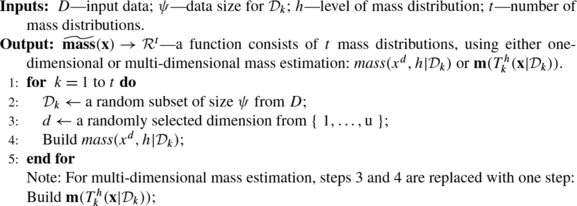

Mass_Estimation(D,ψ,h,t)

C2 :

The second component maps the data set D in the original space of u dimensions into a new data set D′ in t-dimensional mass space using $\widetilde{\mathbf{mass}}(\mathbf{x}) = \mathbf{z}$. This procedure is described in Algorithm 4.

Algorithm 4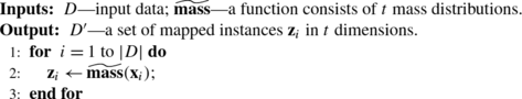

$\mbox{Mass\_Mapping}(D, \widetilde{\mathbf{mass}})$

C3 :

The third component employs a decision rule to determine the final outcome for the task at hand. It is a task-specific decision function applied to z in the new mass space.

The formalism becomes a blueprint for different tasks. Components C1 and C3 are mandatory in the formalism, but component C2 is optional, depending on the task.

For information retrieval and regression, the task-specific C3 procedure is simply using an existing algorithm for the task except that the process is carried out in the new mapped mass space, instead of the original space. The MassSpace procedure is given in Algorithm 5.

Algorithm 5

Perform task in MassSpace(D,ψ,h,t)

The task-specific C3 procedure for anomaly detection is shown in steps 2–5 in Algorithm 6: MassAD. Note that anomaly detection requires C1 and C3 only; whereas the other two tasks require all three components.

Algorithm 6

for Anomaly Detection: MassAD(D,ψ,h,t)

In our experiments described in the next section, the mapping from u dimensions to t dimensions using Algorithm 3 is carried out one dimension at a time when using one-dimensional mass estimation; and all u dimensions at a time when using multi-dimensional mass estimation. Each such mapping produces one dimension in mass space and is repeated t times to get a t-dimensional mass space. Note that randomisation gives different variations to each of the t mappings. The first randomisation occurs at step 2 in Algorithm 3 in selecting a random subset of data. Additional randomisation is applied to attribute selection at step 3 in Algorithm 3 for one-dimensional mass estimation, or at step 4 in Algorithm 2 for multi-dimensional mass estimation.

6 Experiments

We evaluate the performance of MassSpace and MassAD for three tasks in the following three subsections. We denote an algorithm A using one-dimensional and multi-dimensional mass estimations as A′ and A″, respectively.

In information retrieval and regression tasks, the mass estimation uses ψ=8 and t=1000. These settings are obtained by examining the rank correlation as shown in Fig. 4(b)—having a high rank correlation between mass(x,1) and $\mathit{mass}(x,1|\mathcal{D})$. Note that this is done before any method is applied, and no further tuning of the parameters is carried out after this step. In anomaly detection tasks, ψ=256 and t=100 are used so that they are comparable to those used in a benchmark method for a fair comparison. In all tasks, h=1 is used for one-dimensional mass estimation, and it cannot afford to use a high h because of its high cost O(ψ ^h). h=ψ is used for multi-dimensional mass estimation in order to reduce one parameter setting.

All the experiments were run in Matlab and conducted on a Xeon processor which ran at 2.66 GHz and with 48 GB memory. The performance of each method was measured in terms of task-specific performance measure and runtime. Paired t-tests at 5 % significance level were conducted to examine whether the difference in performance is significant between two algorithms under comparison.

Note that we treated information retrieval and anomaly detection as unsupervised learning tasks. Classes/labels in the original data were used as ground truth for evaluation of performance only; they were not used in building mass distributions. In regression, only the training set was used to build mass distributions in step 1 of Algorithm 5; the mapping in step 2 was conducted for both the training and testing sets.

6.1 Content-based image retrieval

We use a Content-Based Image Retrieval (CBIR) task as an example of information retrieval. The MassSpace approach is compared with three state-of-the-art CBIR methods that deal with relevance feedbacks: a manifold based method MRBIR (He et al. 2004), and two recent techniques for improving similarity calculation, i.e., Qsim (Zhou and Dai 2006) and InstR (Giacinto and Roli 2005); and we employ the Euclidean distance to measure the similarity between instances in these two methods. The default parameter settings are used for all these methods.

Our experiments were conducted using the COREL image database (Zhou et al. 2006) of 10000 images, which contains 100 categories and each category has 100 images. Each image is represented by a 67-dimensional feature vector, which consists of 11 shape, 24 texture and 32 color features. To test the performance, we randomly selected 5 images from each category to serve as the queries. For a query, the images within the same category were regarded as relevant and the rest were irrelevant. For each query, we continued to perform up to 5 rounds of relevance feedback. In each round, 2 positive and 2 negative feedbacks were provided. This relevance feedback process was also repeated 5 times with 5 different series of feedbacks. Finally, the average results with one query and in different feedback rounds were recorded. The retrieval performance was measured in terms of Break-Even-Point (BEP) (Zhou and Dai 2006; Zhou et al. 2006) of the precision-recall curve. The online processing time reported is the time required in each method for a query plus the stated number of feedback rounds. The reported result is an average over 5×100 runs for query only; and an average over 5×100×5 runs for query plus feedbacks. The offline costs of constructing the one-dimensional mass estimation and the mapping of 10000 images were 0.27 and 0.32 seconds, respectively. The multi-dimensional mass estimation and the corresponding mapping took 1.72 and 5.74 seconds, respectively.

The results are presented in Table 2 where the retrieval performance better than that conducted in the original space at each round has been boldfaced. The results are grouped for ease of comparison.

Table 2 CBIR results (in BEP×10⁻²). An algorithm A using one-dimensional and multi-dimensional mass estimations are denoted as A′ and A″, respectively. Note that a high BEP is better than a low BEP

The BEP results clearly show that the MassSpace approach achieves a better retrieval performance than that using the original space in all three methods MRBIR, Qsim and InstR, for one query and all rounds of relevance feedbacks. Paired t-tests with 5 % significance level also indicate that the MassSpace approach significantly outperforms each of the three methods in all experiments, without exception. These results show that the mass space provides useful additional information that is hidden in the original space.

The results also show that the multi-dimensional mass estimation provides better information than the one-dimensional mass estimation—MRBIR″, Qsim″ and InstR″ give better retrieval performance than MRBIR′, Qsim′ and InstR′, respectively; only some exceptions occur in the higher feedback rounds for InstR′, with minor differences.

The processing time for the MassSpace approach is expected to be longer than each of the three methods because the number of dimensions in the mass space is significantly higher than those in the original space, where t=1000 and u=67. Despite that, Table 3 shows that MRBIR″, MRBIR′ and MRBIR all have similar level of runtime.

Table 3 CBIR results (online time cost in seconds)

Figure 8 shows an example of performance for InstR′—BEP increases as t increases until it reaches a plateau at some t value; and the processing time is linear w.r.t. the number of dimensions of the mass space, t.

Fig. 8

An example of CBIR round 5 result: The retrieval performance and the processing time as t increases for InstR′

6.2 Regression

In this experiment, we compare support vector regression (Vapnik 2000) that employs the original space (SVR) with that employs the mapped mass space (SVR″ and SVR′). SVR is the ϵ-SVR algorithm with RBF kernel, implemented by LIBSVM (Chang and Lin 2001). SVR is chosen here because it is one of the top performing models.

We utilize five benchmark data sets including four selected from UCI repository (Asuncion and Newman 2007) and one earthquake data (Simonoff 1996) from www.cs.waikato.ac.nz/ml/weka/distribution. The data sizes are shown in the second column of Table 4. We only considered data sets with more than 1000 data points, that contained only real-valued attributes and that had no missing values. we did this in order to get a result with a higher confidence than those obtained from small data sets.

Table 4 Regression results (the smaller the better for MSE)

In each data set, we randomly sampled two-thirds of the instances for training and the remaining one-third for testing. This was repeated 20 times and we report the average result of these 20 runs. The data set, whether in the original space or the mass space, was min-max normalized before an ϵ-SVR model was trained. To select optimal parameters for the ϵ-SVR algorithm, we conducted a 5-fold cross validation based on mean squared error using the training set only. The kernel parameter γ was searched in the range {2⁻¹⁵,2⁻¹³,2⁻¹¹,…,2³,2⁵}; the regularization parameter C in the range {0.1,1,10}, and ϵ in the range {0.01,0.05,0.1}. We measured regression performance in terms of mean squared error (MSE) and runtime in seconds. The runtime reported is the runtime for SVR only. The total cost of mass estimation (from the training set) and mapping (of training and testing sets) in the largest data set, tic, was 1.8 seconds for one-dimensional mass estimation, and 8.5 seconds for multi-dimensional mass estimation. The cost of normalisation and the parameter search using 5-fold cross-validation was not included in the reported result for all SVR″, SVR′ and SVR.

The result is presented in Table 4. SVR′ performs significantly better than SVR in all data sets in MSE measure; the only exception is in the wine_red data set. SVR″ performs significantly better than SVR in all data sets, without exceptions. SVR″ generally performs better than SVR′.

Although both SVR″ and SVR′ take more time to run because each of them runs on the data with a significantly higher dimension, yet the factor of increase in time (shown in the last three columns of Table 5) ranges from 1.3 to 3.4 only, when the factor of increase in the number of dimensions ranges from 12 to over 300. This is because the time complexity in the key optimisation process in SVR is not dependent on the number of dimensions.

Table 5 Regression results (time in seconds)

6.3 Anomaly detection

This experiment compares MassAD with four state-of-the-art anomaly detectors: isolation forest or iForest (Liu et al. 2008), a distance-based method ORCA (Bay and Schwabacher 2003), a density-based method LOF (Breunig et al. 2000), and one-class support vector machine (or 1-SVM) (Schölkopf et al. 2000). MassAD was built with t=100 and ψ=256, the same default settings as used in iForest (Liu et al. 2008), which also employed a multi-model approach. The parameter settings employed for ORCA, LOF and 1-SVM were as stated by Liu et al. (2008).

All the methods were tested on the eight largest data sets used by Liu et al. (2008). The data characteristics are summarized in Table 6, which include one anomaly data generator Mulcross (Rocke and Woodruff 1996) and the other seven are from UCI repository (Asuncion and Newman 2007). The performance was evaluated in terms of averaged AUC (area under ROC curve) and processing time (a total of training time and testing time) over ten runs (following Liu et al. 2008).

Table 6 Data characteristics of the data sets in anomaly detection tasks. The percentage in brackets indicates the percentage of anomalies

MassAD and iForest were implemented in Matlab and tested on a Xeon processor ran at 2.66 GHz. LOF was written in Java in ELKI platform version 0.4 (Achtert et al. 2008); and ORCA was written in C++ (www.stephenbay.net/orca/). The results for ORCA, LOF and 1-SVM were conducted using the same experimental setting but on a slightly slower 2.3 GHz machine, the same machine used by Liu et al. (2008).

The AUC values of all the compared methods are presented in Table 7 where the figures boldfaced are the best performance for each data set. The results show that MassAD using the multi-dimensional mass estimation achieves the best performance in four data sets, and close to the best (the difference which is less than 0.03 AUC) in two data sets; MassAD using the one-dimensional mass estimation achieves the best performance in three data sets, and close to the best in one data set. iForest performs best in four data sets. The results are close for these three algorithms because they share many similarities (see Sect. 9 for details).

Table 7 AUC values for anomaly detection

Again, the multi-dimensional version of MassAD generally performs better than the one-dimensional version, with five wins, one draw and two losses. Most importantly, the worst performance in the Mulcross data set can be easily ‘corrected’ using a better parameter setting—by using ψ=8, instead of 256, the multi-dimensional version of MassAD improves its detection performance from 0.26 to 1.00 in terms of AUC.⁴

It is also noteworthy that the multi-dimensional MassAD significantly outperforms the traditional density-based, distance-based and SVM anomaly detectors in all data sets, except two: one in Annthyroid when compared to ORCA; the poor performance in Mulcross was discussed earlier. The above observations validate the effectiveness of our proposed mass estimation on anomaly detection tasks.

Table 8 shows the runtime result. Although MassAD was run on a slightly faster machine, the result still shows that it has a significant advantage in term of processing time over ORCA, LOF and 1-SVM. The comparison with iForest is presented in Table 9 with a breakdown of training time and testing time. Note that one-dimensional MassAD took the same time as iForest in training, but it only took about one-tenth of the time required by iForest in testing. On the other hand, the multi-dimensional MassAD took slightly more time than iForest in training, but it took up to three times the time required by iForest in testing.

Table 8 Runtime (second) for anomaly detection

Table 9 Training time and testing time (second) for MassAD and iForest, using t=100 and ψ=256

The time and space complexities for five anomaly detection methods are given in Table 10. The one-dimensional MassAD and iForest have the best time and space complexities due to their ability to use small ψ≪n and h=1. Note that the one-dimensional MassAD (h=1) is faster by a factor of log(ψ=256)=8 which shows up in the testing time—ten times faster than iForest given in Table 9. The training time disadvantage, compared to iForest, did not show up because of small ψ. The one-dimensional MassAD also has an advantage over iForest in space complexity by a factor of log(ψ). The multi-dimensional MassAD has similar order of worst-case time and space complexities as iForest, though it might have a larger constant.

Table 10 A comparison of time and space complexities. The time complexity includes both training and testing. n is the given data set size and u is the number of dimensions. For MassAD and iForest, the first part of the summation is the training time and the second the testing time

In contrast to ORCA and LOF (distance-based and density-based methods), the time complexity (and the space complexity) for both MassAD and iForest are independent of the number of dimension u.

6.4 Constant time and space complexities

In this section, we show that $\mathit{mass}(x,h|\mathcal{D})$ (in step 4 of Algorithm 3) takes only constant time, regardless of the given data size n, when the algorithmic parameters are fixed. Table 11 reports the runtime time for sampling (to get a random sample of size ψ from the given data set—steps 2 and 3 of Algorithm 3) and the runtime for one-dimensional mass estimation—to construct $\mathit{mass}(x,h|\mathcal{D})$ t times, for five data sets which include the largest and smallest data sets in regression and anomaly detection tasks.

Table 11 Runtime (second) for sampling, $\mathit{mass}(x,1|\mathcal{D})$ and $\mathit{mass}(x,3|\mathcal{D})$, where t=1000 and ψ=8

The results show that the sampling time increased linearly with the size of the given data set, and it took significantly longer (in the largest data set) than the time to construct the mass distribution—which was constant, regardless of the given data size. Note that the training time provided in Table 9 includes both the sampling time and mass estimation time, and it is dominated by the sampling time for large data sets.

The memory required for each construction of $\mathit{mass}(x,h|\mathcal{D})$ is to store one lookup table of size ψ which is constant.

The constant time and space complexities apply to multi-dimensional mass estimation too.

6.5 Runtime comparison between one-dimensional and multi-dimensional mass estimations

In terms of runtime, the comparison so far in the experiments might give the impression that multi-dimensional mass estimation is worse than one-dimensional mass estimation. In fact, the opposite is true because the above results are obtained from h=1 for one-dimensional mass estimation and h=ψ for multi-dimensional mass estimation. Figure 9 shows the head-to-head comparison for different h values in the COREL data set. When h increases from 1 to 5, the runtime for the one-dimensional mass estimation increases by a factor of 33. In contrast, the runtime for the multi-dimensional mass estimation increases by a factor of 1.5 only.

Fig. 9

Runtime comparison: One-dimensional mass estimation versus multi-dimensional mass estimation for different values of h in the COREL data set, where both are using ψ=8 and t=1000. In this experiment, we set h to the required value for multi-dimensional mass estimation, rather than h=ψ which was used in all experiments reported in the previous sections

6.6 Summary

The above results in all three tasks show that the orderings provided by mass distributions deliver additional information about the data that would otherwise hidden in the original features. The additional information, which accentuates fringe points with a concave function (or an approximation to a concave function in the case of multi-dimensional mass estimation), improves the task-specific performance significantly, especially in the information retrieval and regression tasks.

Using Algorithm 5 for the information retrieval and regression tasks, the runtime is expected to be higher because the new space has much higher dimensions than the original space (t≫u). It shall be noted that the runtime increase (linearly or worse) is solely a characteristic of the existing algorithms used, and is not due to the mass space mapping which has constant time and space complexities.

We believe that a more tailored approach that better integrates the information provided by mass (into the C3 component in the formalism) for a specific task can potentially further improve the current level of performance in terms of either task-specific performance measure or runtime. We have demonstrated this ‘direct’ application using Algorithm 6 for the anomaly detection task, in which MassAD performs equally well or significantly better than four state-of-the-art methods in terms of task-specific performance measure, and the one-dimensional mass estimation executes faster than all other methods in terms of runtime.

Why does one-dimensional mapping work when tackling multi-dimensional problems? We conjecture that if there is no or little interaction between features, then the one-dimensional mapping will work because the ordering that accentuates the fringe points for each original dimension making it easy for existing algorithms to exploit. When there are strong interactions between features, then one-dimensional mapping might not achieve good results. Indeed, our results in all three tasks show that multi-dimensional mass estimation does perform better than one-dimensional mass estimation in general, in terms of task-specific performance measures.

The ensemble method for mass estimation usually needs only a small sample to build each model in an ensemble. In addition, in order to build all t models for an ensemble, tψ could be more than n when ψ>n/t.

The key limitation of the one-dimensional mass estimation is its high cost when a high value of h is applied. This can be avoided by implementing it using a tree structure rather than a lookup table, as we have done using Half-Space Trees which reduces the time complexity to O(th(ψ+n)) from O(t(ψ ^h+1+n)).

7 Relation to kernel density estimation

A comparison of mass estimation and kernel density estimation is provided in Table 12.

Table 12 A comparison of kernel density estimation and mass estimation. Kernel density estimation requires two parameter settings: kernel function K(⋅) and bandwidth h _w ; mass estimation has one: h

Like kernel estimation, mass estimation at each point is computed through a summation of a series of values from a mass base function m _i (⋅), equivalent to a kernel function K(⋅). The two methods differ in the following ways:

• Aim: Kernel estimation is aimed to do probability density estimation; whereas mass estimation is to estimate an order from the core points to the fringe points.

• Kernel function: While kernel estimation can use different kernel functions for probability density estimation; we doubt that mass estimation requires a different base function for two reasons. First, a more sophisticated function is unlikely to provide a better ordering than a simple rectangular function. Second, the rectangular function keeps the computation simple and fast. In addition, a kernel function must be fixed (i.e., having user-defined values for its parameters); e.g., the rectangular kernel function has fixed width or fixed per unit size. But the rectangular function used in mass has no parameter and no fixed width.

• Sample size: Kernel estimation or other density estimation methods require a large sample size in order to estimate the probability accurately (Duda et al. 2001). Mass estimation using $\mathit{mass}(x,h|\mathcal{D})$ needs only a small sample size in an ensemble to accurately estimate the ordering.

Here we present the results using a Gaussian kernel density estimation, replacing the one-dimensional mass estimation, using the same subsample size in an ensemble approach. The bandwidth parameter is set to be the standard deviation of the subsample; and all the other parameters are the same.

The results for information retrieval and anomaly detection are provided in Tables 13 and 15. Compared to mass, density performed significantly worse in information retrieval tasks in all experiments using Qsim and InstR, denoted as Qsim ^K and InstR ^K, respectively. They were even worse than those run in the original space. In anomaly detection, DensityAD, which used a Gaussian kernel density estimation, performed significantly worse than MassAD in six out of eight data sets in the anomaly detection tasks, and better in the other two data sets.

Table 13 CBIR results (in BEP×10⁻²)

8 Relation to data depth

There is a close relationship between the proposed mass and data depth (Liu et al. 1999): they both delineate the centrality of a data cloud (as opposed to compactness in the case of the density measure). The properties common to both measures are: (a) the centre of a data cloud has the maximum value of the measure; (b) an ordering from the centre (having the maximum value) to the fringe points (having the minimum values).

However, there are two key differences. First, not until recently (see Agostinelli and Romanazzi 2011) data depth always models a given data with one centre, regardless whether the data is unimodal or multi-modal; whereas mass can model both unimodal and multi-modal data by setting h=1 or h>1. Local data depth (Agostinelli and Romanazzi 2011) has a parameter (τ) which allows it to model multi-modal data as well as unimodal data. However, the performance of local data depth appears to be sensitive to the setting of τ (see a discussion of the comparison below). In contrast, a single setting of h in mass estimation had produced good task-specific performance in three different tasks in our experiments.

Second, mass is a simple and straightforward measure, and has efficient estimation methods based on axis-parallel partitions only. Data depth has many different definitions, depending on the construct used to define depth. The constructs could be Mahalanobis, Convex Hull, simplicial, halfspace and so on (Liu et al. 1999), all of which are expensive to compute (Aloupis 2006)—this has been the main obstacle in applying data depth to real applications in multi-dimensional problems. For example, Ruts and Rousseeuw (1996) compute the contour of data depth of a data cloud for visualization, and employ depth as the anomaly score to identify anomalies. Because of its computational cost, it is limited to small data size only. In contrast to the axis-parallel partitions used in mass estimation, halfspace data depth⁵ (Tukey 1975), for example, requires to consider all halfspaces which demands high computational time and space.

To provide a comparison, we replace the one-dimensional mass estimation (defined in Algorithm 3) with data depth (defined by simplicial depth Liu et al. 1999) and local data depth (defined by simplicial local depth Agostinelli and Romanazzi 2011). We repeat the experiments by employing both the data depth and local data depth implementation in R by Agostinelli and Romanazzi (2011) (accessible from r-forge.r-project.org/projects/localdepth). Both data depths are carried out in the same approach by using sample size ψ to build each of the t models in an ensemble.⁶ The number of simplices used to do the empirical estimation is set to 10000 for all runs. Default settings are used for all other parameters (i.e., the membership of a data point in simplices is evaluated in the “exact” mode rather than the approximate mode, and the tolerance parameter is fixed to 10⁻⁹). Note that local depth uses an additional parameter τ to select candidate simplices, where a simplex having volume larger than τ is excluded from consideration. As the performance of local depth is sensitive to τ, we employ the quantile order of τ of 10 %, the low value of the range 10 %–30 % suggested by Agostinelli and Romanazzi (2011). Because both data depth and local data depth are estimated using the same procedure, their runtimes are the same.

The task-specific performance result for information retrieval is provided in Table 13. Note that local data depth could produce worse retrieval results than those in the original feature space. Data depth performed close to that achieved by the one-dimensional mass estimation, but it was significantly worse than the multi-dimensional mass estimation.

Figure 10 shows a scale up test in the information retrieval task using Qsim with one query and feedback round 5. It is interesting to note both mass and data depth performed better using small rather than large subsampling size. As expected, KDE produced better results with increasing subsampling sizes; but even with ψ=8196 in the COREL data set of 10000 instances, KDE still performed the worst compared to mass and data depth.

Fig. 10

Scale up test in information retrieval using Qsim. Subsampling data size is increased from ψ=8 to ψ=8196 in the COREL image data set containing 10000 instances. The same experimental setting as reported in Sect. 6.1 is used

Table 15 shows the result in anomaly detection. Data depth performed worse than both versions of mass estimation in six out of eight data sets; local data depth performed worse than multi-dimensional mass estimation in five out of eight data sets; local data depth versus one-dimensional mass estimation have four wins and four losses. Note that though local data depth achieved the best result in two data sets, it also produced the worst in three data sets which were significantly worse than others (in http, forest and shuttle).

The runtime results are provided in Tables 14 and 16. These results do not reveal the time complexities of the algorithms because of small ψ (and the CBIR results do not include the offline time cost). We conducted a scale up test using the Mulcross data set by increasing the subsampling size. Using the runtime at ψ=8 as the base, runtime ratio is computed for all other subsampling sizes. The result is presented in Fig. 11. It shows that data depth or local data depth had the worst runtime ratio which increased its runtime 58 times when ψ was increased by a factor of 512. The multi-dimensional mass estimation had the best runtime ratio of 6.6, followed by KDE (24) and one-dimensional mass estimation (34) when ψ ratio=512. The actual runtimes in seconds were 126.6 (Mass″), 166.7 (KDE), 239.4 (Mass′), and 600.5 (Data Depth). This result is not surprising because the multi-dimensional mass estimation has time complexity O(ψ), KDE has O(ψ ²), the one-dimensional mass estimation has O(ψ ^h+1), and data depth using simplices has O(ψ ⁴) (Aloupis 2006).

Table 14 CBIR results (online time cost in seconds)

Table 15 Anomaly detection: MassAD vs DensityAD and DepthAD (AUC)

Table 16 Anomaly detection: MassAD vs DensityAD and DepthAD (time in seconds)

Fig. 11

Scale up test using the Mulcross data set. The base subsampling data size (ψ) is 8; doubling at each step until ψ=4096. Each point in the graph is an average over 10 runs

9 Other work based on mass

iForest (Liu et al. 2008) and MassAD share some common features: Both are ensemble methods which build t models, each from a random sample of size ψ, and they both combine the outputs of the models through averaging during testing. Although iForest (Liu et al. 2008) employs path length—an instance traverses from the root of a tree to its leaf—as the anomaly score, we have shown that the path length used in iForest is in fact a proxy to mass (see Sect. 4.1 for details). In other words, iForest is a kind of mass-based method—that is why MassAD and iForest have similar detection accuracy. Multi-dimensional MassAD has the closest resemblance to iForest because of the use of tree. The key difference is that MassAD is just one application of the more fundamental concept of mass introduced here, whereas iForest is for anomaly detection only. In terms of implementation, the key difference is how the cut-off value is selected at each internal node of a tree: iForest selects the cut-off value randomly whereas a Half-Space Tree selects a mid point deterministically (see step 5 in Algorithm 2).

How easily can the proposed formalism be applied to other tasks? In addition to the tasks we have applied in this paper, we have applied mass estimation ‘directly’, using the proposed formalism, to solve problems in content-based multimedia information retrieval (Zhou et al. 2012) and clustering (Ting and Wells 2010). While the ‘indirect’ application is straightforward which simply uses the existing algorithms in the mass space, a ‘direct’ application requires a complete rethink of the problem and produces a totally different algorithm. However, this rethink of a problem in terms of mass often results a more efficient and sometimes more effective algorithm than existing algorithms. We provide a brief description of the two applications in the following two paragraphs.

In addition to the mass-space mapping we have shown here (i.e., components C1 and C2), Zhou et al. (2012) present a content-based information retrieval method that assigns a weight (based on iForest, thus, mass) to each new mapped feature w.r.t. a query; and then it ranks objects in the database according to their weighted average feature values in the mapped space. The method also incorporates relevance feedback which modifies the ranking based on the feedbacks through reweighted features in the mapped space. This method forms the third component of the formalism stated in Sect. 5. This ‘direct’ application of mass has been shown to be significantly better than the ‘indirect’ approach we have shown in Sect. 6.1, in terms of both task-specific measure and runtime (Zhou et al. 2012). It is interesting to note that, unlike existing retrieval systems which rely on a metric, the new mass-based method does not employ a metric—it is the first information retrieval system that does not use a metric, as far as we know.

Ting and Wells (2010) use a variant of Half-Space Trees we have employed here and apply mass directly to solve clustering problems. It is the first mass-based clustering algorithm, and it is unique because it does not use any distance and density measure. In this task, like in the case of anomaly detection, only two components are required. After building a mass model (in the C1 component), the C3 component consists of linking instances with non-zero mass connected by the mass model and making each group of connected instances a separate cluster; and all other unconnected instances are regarded as noise. This mass-based clustering algorithm has been shown to perform equally well as DBSCAN (Ester et al. 1996) in terms of clustering performance, but it runs orders of magnitude faster (Ting and Wells 2010).

The earlier version of this paper (Ting et al. 2010) establishes the properties of mass estimation in the one-dimensional setting only; and use it in all three tasks. This paper extends one-dimensional mass estimation to multi-dimensional mass estimation using the same approach as described by Ting and Wells (2010), and implements multi-dimensional mass estimation using Half-Space Trees. This paper reports new experiments using the multi-dimensional mass estimation, and shows the advantage of using multi-dimensional mass estimation over one-dimensional mass estimation in the three tasks reported earlier (Ting et al. 2010). These related works show that mass estimation can be implemented in different ways using tree-based or non-tree-based methods.

10 Conclusions and future work

This paper makes two key contributions. First, we introduce a base measure, mass, and delineate its three properties: (i) a mass distribution stipulates an ordering from core points to fringe points in a data cloud; (ii) this ordering accentuates the fringe points with a concave function—a property that can be easily exploited by existing algorithms to improve their task-specific performance; and (iii) the mass estimation methods have constant time and space complexities. Density estimation has been the base modelling mechanism employed in many techniques thus far. Mass estimation introduced here provides an alternative choice, and it is better suited for many tasks which require an ordering rather than probability density estimation.

Second, we present a mass-based formalism which forms a basis to apply mass to different tasks. The three tasks (i.e., information retrieval, regression and anomaly detection) to which we have successfully applied are just examples of its application. Mass estimation has potentials in many other applications.

There are potential extensions to the current work. First, the algorithms for the three tasks and the formalism can be improved or extended to include more tasks. Second, because the purposes and their properties differ, mass estimation is not intended to replace density estimation—it is thus important to identify areas in which each is best suited for. This will ascertain (i) areas in which density has been a mismatch, unbeknown up to now, and (ii) areas in which mass estimation is weak. Third, the proposed approach to multi-dimensional mass estimation is an approximation and it does not guarantee concavity. It will be interesting to explore a version that has such a guarantee and to examine whether it will further improve the task-specific performance in all three tasks reported here. Fourth, the current implementation of multi-dimensional mass estimation using Half-Space Trees limits its applications to low dimensional problems because it suffers the same problem as in all other grid oriented methods. We will explore non-grid oriented implementations of mass which have potential to tackle high dimensional problems more effectively than existing density-based and distance-based methods.

Appendix: Anomaly detection using data depth that builds a single model from the entire data set

This appendix provides the results in anomaly detection task where data depth and local data depth built a single model from the entire data set, i.e., DepthAD _s . This is in contrast to DepthAD which employed an ensemble approach in Sect. 8.

Table 17 shows that MassAD generally has higher AUC than DepthAD _s which employed either data depth or local data depth. The only exception is the Annthyroid data set. Note that these results are generally worse than those employing an ensemble approach, reported in Table 15.

Table 17 AUC values for anomaly detection, comparing MassAD with DepthAD _s (which employed either data depth or local data depth) that build a single model from the entire data set

References

Achtert, E., Kriegel, H.-P., & Zimek, A. (2008). ELKI: a software system for evaluation of subspace clustering algorithms. In Proceedings of the 20th international conference on scientific and statistical database management (pp. 580–585).
Agostinelli, C., & Romanazzi, M. (2011). Local depth. Journal of Statistical Planning and Inference, 141, 817–830.
Aloupis, G. (2006). Geometric measures of data depth. DIMACS Series in Discrete Math and Theoretical Computer Science, 72, 147–158.
Asuncion, A., & Newman, D. (2007). UCI machine learning repository.
Bay, S. D., & Schwabacher, M. (2003). Mining distance-based outliers in near linear time with randomization and a simple pruning rule. In Proceedings of ACM SIGKDD (pp. 29–38).
Breunig, M. M., Kriegel, H.-P., Ng, R. T., & Sander, J. (2000). LOF: identifying density-based local outliers. In Proceedings of ACM SIGKDD (pp. 93–104).
Chang, C.-C., & Lin, C.-J. (2001). LIBSVM: a library for support vector machines.
Duda, R., Hart, P., & Stork, D. (2001). Pattern classification (2nd ed.). New York: Wiley.
Ester, M., Kriegel, H.-P., Sander, J., & Xu, X. (1996). A density-based algorithm for discovering clusters in large spatial databases with noise. In Proceedings of ACM SIGKDD (pp. 226–231).
Giacinto, G., & Roli, F. (2005). Instance-based relevance feedback for image retrieval. In Advances in NIPS (pp. 489–496).
He, J., Li, M., Zhang, H., Tong, H., & Zhang, C. (2004). Manifold-ranking based image retrieval. In Proceedings of ACM multimedia (pp. 9–16).
Liu, F. T., Ting, K. M., & Zhou, Z.-H. (2008). Isolation forest. In Proceedings of IEEE ICDM (pp. 413–422).
Liu, R., Parelius, J. M., & Singh, K. (1999). Multivariate analysis by data depth. The Annals of Statistics, 27(3), 783–840.
Quinlan, J. (1993). C4.5: programs for machine learning. San Mateo: Morgan Kaufmann.
Rocke, D. M., & Woodruff, D. L. (1996). Identification of outliers in multivariate data. Journal of the American Statistical Association, 91(435), 1047–1061.
Ruts, I., & Rousseeuw, P. (1996). Computing depth contours of bivariate point clouds. Computational Statistics and Data Analysis, 23(1), 153–168.
Schölkopf, B., Williamson, R. C., Smola, A. J., Shawe-Taylor, J., & Platt, J. C. (2000). Support vector method for novelty detection. In Advances in NIPS (pp. 582–588).
Simonoff, J. S. (1996). Smoothing methods in statistics. Berlin: Springer.
Ting, K. M., & Wells, J. R. (2010). Multi-dimensional mass estimation and mass-based clustering. In Proceedings of IEEE ICDM (pp. 511–520).
Ting, K. M., Zhou, G.-T., Liu, F. T., & Tan, S. C. (2010). Mass estimation and its applications. In Proceedings of ACM SIGKDD (pp. 989–998).
Tukey, J. W. (1975). Mathematics and picturing data. In Proceedings of the international congress on mathematics (Vol. 2, pp. 525–531).
Vapnik, V. N. (2000). The nature of statistical learning theory (2nd ed.). Berlin: Springer.
Zhang, R., & Zhang, Z. (2006). BALAS: empirical Bayesian learning in the relevance feedback for image retrieval. Image and Vision Computing, 24(3), 211–223.
Zhou, G.-T., Ting, K. M., Liu, F. T., & Yin, Y. (2012). Relevance feature mapping for content-based multimedia information retrieval. Pattern Recognition, 45, 1707–1720.
Zhou, Z.-H., Chen, K.-J., & Dai, H.-B. (2006). Enhancing relevance feedback in image retrieval using unlabeled data. ACM Transactions on Information Systems, 24(2), 219–244.
Zhou, Z.-H., & Dai, H.-B. (2006). Query-sensitive similarity measure for content-based image retrieval. In Proceedings of IEEE ICDM (pp. 1211–1215).
Zuo, Y., & Serfling, R. (2000). General notion of statistical depth function. The Annal of Statistics, 28, 461–482.
Acknowledgements
This work is supported by the Air Force Research Laboratory, under agreement numbers FA2386-09-1-4014, FA2386-10-1-4052 and FA2386-11-1-4112. The US Government is authorized to reproduce and distribute reprints for Governmental purposes notwithstanding any copyright notation thereon. The anonymous reviewers have provided many helpful comments to improve the clarity of this paper.
Author information
Authors and Affiliations
Corresponding author
Additional information
Editor: Tong Zhang.