
Abstract
Unstable friction-induced vibrations are considered an annoying problem in several fields of engineering. Although several theoretical analyses have suggested that friction-excited dynamical systems may experience sub-critical bifurcations, and show multiple coexisting stable solutions, these phenomena need to be proved experimentally and on continuous systems. The present work aims to partially fill this gap. The dynamical response of a continuous system subjected to frictional excitation is investigated. The frictional system is constituted of a 3D printed oscillator, obtained by additive manufacturing that slides against a disc rotating at a prescribed velocity. Both a finite element model and an experimental setup has been developed. It is shown both numerically and experimentally that in a certain range of the imposed sliding velocity the oscillator has two stable states, i.e. steady sliding and stick–slip oscillations. Furthermore, it is possible to jump from one state to the other by introducing an external perturbation. A parametric analysis is also presented, with respect to the main parameters influencing the nonlinear dynamic response, to determine the interval of sliding velocity where the oscillator presents the two stable solutions, i.e. steady sliding and stick–slip limit cycle.
1 Introduction
Friction-induced vibrations (FIV) [1] are ubiquitous in mechanics and unstable FIV are considered a common problem in several fields of engineering, ranging from automotive [2], railways industry [3], aerospace [4,5,6,7] and bioengineering [8, 9]. The problem is very widespread as in engineering applications almost all mechanical systems are assembled together and include contacting interfaces, e.g. joints [8, 10, 11], dampers and brake systems [12,13,14]. High amplitude FIV is commonly the consequences of friction instabilities that give rise to tedious noise [15,16,17,18] usually classified in squeal, groan or chatter depending on the frequency band in which it occurs [19]. One of the phenomena at the origins of such noises are stick–slip [20]. The appearance of stick–slip instability is influenced by the combination of several tribological and dynamical processes and parameters [21, 22], which in real systems are difficult to discern. One cause of instability is a falling characteristic of the friction coefficient with the relative velocity that may lead to negative damping, causing stick–slip oscillations [23,24,25]. Another kinematic explanation for FIV is the so called sprag-slip instability, which is caused by “jamming” at the interface level [26]. Lastly, “flutter” (or mode-coupling) is an instability mechanism which emerge when, while changing a system parameter, two stable modes merge giving rise to one stable and one unstable mode [27]. Not only the sliding velocity but also damping plays a fundamental role for the occurrence of instability. It has been shown [28, 29] that the increase in the overall system damping allows a smoother transition from micro-slips to continuous sliding. Although several authors have studied the problem of FIV, it remains today a challenge to confidently predict the appearance of FIV, mostly due to the inherent nonlinearity involved in the analysis. Indeed the contact stiffness is generally nonlinear [30] and the friction law is often multivalued even in the most simple Coulomb model [31]. Several authors have shown that due to the system nonlinearity, the frictional system may experience subcritical Hopf bifurcations, with multiple co-existing stable states, i.e. full sliding and stick–slip vibrations [23, 32,33,34]. Papangelo and co-authors [35] considered a mass-spring-damper system in contact with a moving belt with velocity weakening characteristic of the friction law. They showed that a certain region of belt velocity exists, where two attractors are observed: a steady-sliding solution, where small oscillations are damped, and a stick–slip high amplitude limit cycle, being the system state selected by the initial conditions. The authors showed that the width of the bi-stable region is reduced by decreasing the ratio static (μs) to dynamic (μd) friction coefficient or by considering a strengthening term in the friction law. Similar results have been obtained in alike lumped systems [36] using a simple discontinuous Coulomb friction law with μs > μd. For the chosen parameters, the investigated system becomes linearly unstable under small oscillations above a critical friction coefficient, but stick–slip limit cycle oscillations continue to exist (when μs/μd > 1) even for smaller velocities. In multiple degrees of freedom system, vibration localization may occur in certain regions of the governing parameters, where multiple stable co-existing solutions exist [34, 37]. Although several authors have attempted to study experimentally the nonlinearity of FIV, most of the literature results focus on lumped systems (typically a concentrated mass connected to springs and dampers and generally sliding on a substrate). In general, such models do not face the problem of the co-existence of multiple dynamical states, assuming the solution “a regime” is unique for a given set of system parameters [38, 39]. Nevertheless multiple states have been experimentally measured in mass-on-moving-belt lumped systems by Saha et al. [40] and in a brake apparatus by Gräbner et al. [41].
In the present work, a continuous oscillating system in contact with a moving disk is investigated numerically and experimentally to demonstrate the existence of the bi-stable region. Numerical simulations of multiple coexisting dynamical states are shown for the same imposed velocity. An experimental setup has been developed, and parametrical studies have been performed to characterize the region of parameters for which multiple dynamical equilibria coexist.
2 Methodology
As mentioned above, few contributions in literature deal with bi-stable dynamical states in continuous frictional systems. In this work the geometry shown in Fig. 1, obtained experimentally by additive manufacturing, is used to analyse the nonlinear behaviour of stick–slip instability. The proposed geometry is a frictional oscillator, clamped at one side and in frictional contact on the other one with a rigid steel disc. Because the oscillator used in the experimental campaign has been obtained by additive manufacturing, the material properties are slightly different from those of common steel material. While the density (7450 kg/m3) has been calculated by its volume and weight, the Young’s Modulus (131 GPa) has been calculated by comparing its natural frequencies, obtained experimentally and numerically.

a Geometry of the oscillator obtained by additive manufacturing; b oscillator in contact with the disc with an inclination angle α
As multiple stable solutions exist for a certain sliding velocity, it is of outmost importance to clearly define the loading protocol used in both the numerical and experimental analysis:
-
1.
The normal load is first imposed by applying a vertical displacement at the clamped end of the oscillator; the imposed vertical displacement is kept constant during the entire test.
-
2.
The relative velocity between the oscillator and the disc is increased up to a certain target velocity. This phase is referred as the “acceleration phase” (see Fig. 2 and Table 2).
Fig. 2 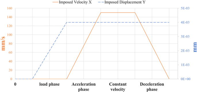
Example of the imposed displacement and velocity profile both numerically and experimentally
-
3.
The velocity of the disc is kept constant for a certain time.
-
4.
The disc velocity is decreased up to the rest. This phase is referred to as the “deceleration phase”.

This trapezoidal profile (see Fig. 2) of the imposed velocity allows for the determination of the so called “critical velocities” [35], i.e. the values of the imposed velocity at which the system switches from stick–slip to stable sliding and vice versa, when, respectively, the system is either accelerating or decelerating. The control parameter for switching from one state to another is then the imposed velocity of the disc.
The aim is to retrieve, as obtained numerically in lumped models [34, 35], the presence of the bi-stable region, and to study the effects of the variation of the key parameters. While numerically the effect of the friction coefficients is investigated, the experiments allow for investigating the effect of the inclination angle and normal load.
3 Numerical analysis
3.1 Finite element model and frictional behaviour
A finite element model of the oscillator in contact with the disc (Fig. 1) was developed using the commercial code ANSYS WORKBENCH. To reduce the computational cost of a full transient frictional dynamical simulation, we have exploited the symmetry of the geometry to develop a 2D numerical model (Fig. 3). Figure 3 shows the numerical model with the imposed boundary conditions. The upper part of the oscillator is constrained along the x-direction, while the normal load is applied by imposing a displacement in the vertical direction. The disc, instead, is constrained in the vertical direction and can move in the horizontal direction with a prescribed velocity profile (see Fig. 2). In order to accurately model the contact zone, the mesh is refined close to the contact interface up to an element size of about 25 µm side length.

2D numerical model (plane strain) with imposed boundary conditions and zoom on mesh refinement in the contact area. System acceleration along X-direction is recovered at point A
The friction law is introduced in the numerical simulation by the definition of the µs/µd ratio (a) and a decay constant (d), according to the following exponentially decaying law:
If zero is set as value for d, the exponential law reduces to a sudden drop, so that there is a discontinuous transition from the static to the dynamic friction coefficient in the transition from sticking to sliding.
The transient simulation is solved by using implicit Newmark time integration scheme [42], with a time step of 1e−5 s and a number of 42,200 nodes. The pure penalty method is implemented at the contact interface, in both normal and tangential directions.
3.2 Nonlinear frictional response
The numerical model is here implemented to reproduce numerically the existence of the bi-stable region. Then, the effect of the friction coefficients, a parameter that cannot be easily varied experimentally, is investigated in the occurrence of the instability and the bi-stable velocity interval. It should be kept in mind that the imposed velocity and acceleration are higher than in the experiments (see Sect. 4). This is due to the need in reducing the overall computational time in simulating a nonlinear transient finite element analysis. Nevertheless, the objective is to verify if the bi-stable region is retrieved and to highlight the trend with respect to the friction parameters. The experiments will then allow for retrieving the same data with more realistic acceleration values. At this first stage, the friction law has been set with a nil value for the decay constant d, so that the focus has been set on the effect of the ratio between static and dynamic friction coefficients. Figure 4 shows the results of the transient simulation obtained with µs equal to 0.4 and µd equal to 0.2. In the beginning of the acceleration phase, the oscillator experiences stick–slip limit cycle oscillations. At a velocity of about \( \sim \) 110 mm/s there is a sudden drop in the horizontal acceleration signal, which indicates a transition to steady sliding. The disc velocity reaches a maximum of 150 mm/s, is kept constant for 0.1 s, then starts to decrease. While the disc decelerates, steady sliding remains stable up to about \( \sim3 \) 0 mm/s, then for lower velocity, stick–slip oscillations take place. The differing “critical velocities” obtained during the acceleration and deceleration phases clearly show that a bi-stable region, with two coexisting stable solutions, have been identified in the numerical results.

Acceleration along the x-direction obtained for a simulation with µs equal to 0.4 and µd equal to 0.2; imposed initial normal load = 30 N/mm
Figure 5 shows the corresponding bifurcation diagram, where the amplitude of the vibration (moving acceleration RMS) is plotted against the driving imposed velocity. The blue dotted curve (circles) is related to the acceleration phase, while the red dotted curve (triangles) is related to the deceleration phase. The following three regions can be observed:

Bifurcation diagram obtained with the acceleration data shown in Fig. 4
-
At high imposed driving velocity stable sliding is observed both in acceleration and deceleration;
-
At lower imposed driving velocity stick–slip is observed both in acceleration and deceleration; the curve in acceleration (dotted-blue) starts at a velocity different from zero (about 27 mm/s) because, when the lower surface starts moving (from 0 to 27 mm/s), the oscillator deforms to reach its equilibrium state before sliding at the interface;
-
The bi-stable zone is obtained, where stick–slip instability and stable sliding solutions coexists; in this region, the system shows stick–slip vibrations when coming from lower velocities (stick–slip initial condition) and shows stable sliding when coming from higher velocities (stable sliding).
The bifurcation diagram shows then that the bi-stable region has been obtained for a continuous system in frictional contact with a moving counterpart.
3.3 Critical velocity versus friction
A parametrical analysis has been then performed to ascertain the effect of the ratio static to dynamic friction coefficient on the velocity interval (difference between upper and lower critical velocity) in which the system exhibits a bi-stable behaviour. The same value of the static and dynamic friction coefficient brings to an overall stable sliding condition. On the other hand, when the two friction values are set different, with higher static friction, the stick–slip instability occurs within different velocity interval. The results are summarised in Table 1 and Fig. 6 for \( \mu_{s} /\mu_{d} \) that ranges between 1.14 and 2.5.

Bi-stable velocity interval as a function of the static/dynamic friction ratio
The first evidence from Table 1 and Fig. 6 is that the ratio between the two friction coefficients determines the spread between the two critical velocities, increasing the length of the velocity interval of the bi-stable region. Another important aspect to notice is that, while the acceleration critical velocity presents large variations according to the change in the ratio between the friction coefficients, the critical velocity in deceleration stays almost constant. Its small variation, instead, seems to be correlated rather with the change in the dynamic friction coefficient: with an increase in µd, a slight increase in the critical velocity in deceleration is observed. The larger increase in the critical velocity in acceleration, with respect to the one in deceleration, according to the µs/µd ratio, has been observed as well numerically on lumped models [35].
4 Experimental results
4.1 Test-bench
A dedicated test bench (Fig. 7), developed for the study of contact instabilities [43,44,45], has been adapted to reproduce the nonlinear dynamic response of the investigated system. The oscillator is put in contact with its counterpart, a steel disc driven by a brushless electric engine, imposing a vertical displacement to its clamped end. The clamping is obtained by a massive block, in order to isolate as much as possible the dynamics of the oscillator [46]. To obtain a better clamping condition and avoid micro sliding at the interface with the clamping block, the upper part of the oscillator has been designed with a thicker section and the corresponding fillet radius (Fig. 7a). Both the normal and the tangential forces are acquired with a 3-axial piezoelectric transducer (Kistler 9017C) located on the upper side of the oscillator. In order to follow the dynamic response of the system, an accelerometer (B&K type 4397) has been positioned at one side of the oscillator, close to the contact interface. A micrometric positioning system is used to apply the load by imposing a vertical displacement to the oscillator, while the inclination angle (see Fig. 1) is obtained by an angular positioning system.

CAD design (a) and photo of the experimental setup (b): (1) vertical support, (2) horizontal support, (3) linear vertical positioning system, (4) 3D force transducer, (5) angular positioning system, (6) massive block, (7) oscillator, (8) disc
The geometry of the oscillator, at the contact side, has been set with two curvature radii (Fig. 7) in order to have a barrel-like shape and ensure the contact in well-localized area in the middle of the oscillator plane, avoiding misalignment issues that would have led to strong asymmetry in the contact zone. The oscillator has been printed by additive technology in steel material.
It order to obtain a frictional response with static friction higher than the dynamic one, the oscillator was coated on the contact side with an epoxy resin. The frictional response of the used epoxy resin in contact with steel material has been measured on a dedicated tribometer [44, 47] to retrieve the friction-velocity characteristic curve, shown in Fig. 8.

4.2 Non-linear stick–slip response
Before the experimental campaign, a running-in phase is required to establish a transfer film of resin on the disc surface, which has been previously polished to obtain a roughness of Ra = 1 µm. After the running-in of the surfaces, the tests have been performed. Figure 9 shows the response of the frictional system during a reference test, where the different phases of the experimental protocol are listed in Table 2. Referring to the imposed boundary conditions (Fig. 2), for the presented test, a vertical displacement is imposed to the system in order to reach an initial load of 50 N, while the maximum speed is set to 44 mm/s.

Recorded acceleration (up) and acceleration spectrogram (down) from an experimental test with angle = 5° and initial load = 50 N
As soon as the relative motion starts (disc rotation), the acceleration of the oscillator shows high amplitude oscillations, until a second stage can be detected, when only low amplitude friction noise is observed. The low amplitude noise increases slightly with the imposed velocity, stays at constant amplitude when the imposed velocity is kept constant, and it decreases again with the decreasing of the velocity, until high amplitude oscillations take place again; here, a sudden increase in the acceleration amplitude occurs and develop until the final stop of the disc.
The low amplitude acceleration is friction noise [46], due to broadband excitation coming from the contact, during the stable sliding state between the oscillator and disc surfaces. The emphasis is here placed on the values of “critical velocities”, i.e. the imposed relative velocities at which the jumps between stable sliding (friction noise) and stick–slip (impulsive oscillations) occur. The impulsive nature of the stick–slip phenomenon is also highlighted in the zoom of the spectrogram in Fig. 9 (when increasing of the imposed velocity); a typical large band excitation (vertical lines) of the system natural frequencies is observed for each periodical stick–slip event. Moreover, increasing the imposed velocity (in the acceleration phase), the period of stick–slip decreases. Then, for higher velocities, the system oscillations are not completely damped between the successive impulsive excitations, leading to continuous oscillations at the natural modes of the system (horizontal lines). The almost continuous lines in the spectrum appears first for the low frequency modes, because they are less damped. Increasing the imposed velocity, the frictional system switches from a stick–slip state to a stable sliding (red star in Fig. 9, v = 13 mm/s) and the spectrogram shows a low amplitude and large band vibrations due to the friction noise. The analogue time and frequency system response is recovered during the deceleration phase (from 40 to 60 s), where the switching from stable sliding to stick–slip state takes place for a lower critical velocity (green star in Fig. 9, v = 7.5 mm/s). In the test reported in Fig. 9, it is possible to observe two different critical velocities for the acceleration phase, at 13 mm/s, and the deceleration phase, at 7.5 mm/s. This proves experimentally that in the velocity interval (7.5–13 mm/s) the system dynamical equilibria can result in stick–slip oscillations (acceleration phase) or in steady sliding (deceleration phase) determining a region of bi-stability, as indeed found in literature for lumped systems [35].
4.3 Parametrical analysis
A parametrical analysis, with respect to the applied normal loadFootnote 1 and the inclination angle of the oscillator, has been performed in order to study the effects of the variation of these parameters. In particular, the normal load is varied between 50 N, upper limit of the positioning system, and 20 N, under which the system does not show appreciable stick–slip instability. On the other hand, the angle has been varied from 5° up to 20°. Tests with higher values do not present stick–slip, while lower inclinations can cause wedging of the oscillator during the test. For each configuration of the angle, all the load values have been tested. Table 3 gives the values of the obtained critical velocities, both in acceleration and deceleration, for each combination of normal load and inclination angle. As expected, when combing lower loads with larger angles the system do not show stick–slip instability (critical velocity equal to 0). When decreasing the angle, or increasing the load, the critical velocities increase (Fig. 10).

a Difference in critical velocities (bi-stable velocity interval) for fixed angle (5°); b Difference in critical velocities for fixed load (50 N)
As well, the overall breadth of the bi-stable velocity interval increases with the increase in load and decrease in the inclination angle (Fig. 10). Being friction and contact instabilities are quite sensitive to several parameters, when comparing the trends of the critical velocities and the by-stability velocity interval, it should be kept in mind that the reported values are not to be taken as absolute. The main results are here the qualitative trends with respect to variations of the selected parameters (Fig. 11).

Experimental parametric results in terms of the bi-stable velocity interval as a function of the initial load and imposed angle
5 Switching within the bi-stable behaviour
In this section the bifurcation diagram, showing the acceleration amplitude RMS as a function of the imposed relative velocity, is reconstructed from the experimental results, and it is shown that it is possible to switch between the two states, i.e. stable sliding and stick–slip, within the bi-stable region by introducing an external perturbation. Figure 12 presents the bifurcation diagram, obtained from the acceleration measured during the experimental test shown in Fig. 9. The curve is obtained performing a moving root mean square (RMS) of the acceleration signal with time window of 0.2 s.

Bifurcation diagram obtained for normal load of 50 N and 5° of inclination angle. The acceleration data are those shown in Fig. 9
During the acceleration branch (blue curve, circles) the stick–slip amplitude increases and then decreases with the increasing of the velocity, to disappear at about 13 mm/s, when stable sliding is observed. In the deceleration branch (red curve, diamonds), instead, the critical speed to switch from stable sliding to stick–slip is at about 7.5 mm/s, highlighting the bi-stable range with the two possible states between 7.5 and 13 mm/s.
The difference in the critical velocities is quite large, allowing performing a new test, at constant velocity, in the region of the bi-stability, as pointed out in Fig. 12. The test begins in steady sliding condition at a constant velocity of 9 mm/s (red dot in Fig. 12), which has been reached starting for high velocity and decelerating the disc. Thus, the system is in stable sliding, showing low amplitude friction noise in the acceleration (Fig. 13, until 32.37 s). After a while, an impulsive excitation has been provided by an external impact on the oscillator (at 9 mm/s in Fig. 12) and the system response shows stick–slip oscillation in the temporal response and remains in this state. The system, excited by an external perturbation, has moved from the stable sliding branch to the unstable stick–slip branch (from red to blue dots in Fig. 12), which shows how the dynamical equilibria in frictional systems may be very sensitive to external perturbations.

Acceleration signal when the system is within the bi-stable zone; an impulsive excitation (up) switches the system response between the two solution branches; load of 50 N, 5° of inclination angle and constant imposed velocity of 9 mm/s
6 Conclusions
In this work, the nonlinear dynamical response of a continuous system subjected to frictional excitation has been studied both experimentally and numerically. Although relevant works in literature have dealt with the topic of friction-induced vibrations, few experimental contributions have been published investigating the multi-stability in frictional systems, i.e. the possibility to show experimentally multiple coexisting dynamical equilibria for the same set of governing parameters. The original contribution of this work, is the extension of such observations and analyses on continuous frictional systems, both numerically and experimentally.
Firstly, a dedicated finite element model of the investigated frictional system has been developed. Then, the frictional oscillator has been realized by additive manufacturing and coated with a layer of epoxy resin that shows a quite reproducible negative friction-velocity slope. Both experiments and numerical results show that, within a certain interval of imposed velocity, the frictional system presents two stable co-existing solutions (stable sliding and stick–slip instability), which are selected by the system initial conditions. Then, the bifurcation diagrams have been traced both numerically and experimentally.
A parametrical analysis has been then performed as a function of the normal load, inclination angle and friction coefficients, showing that the width of the bi-stable regime reduces by reducing the ratio static to dynamic friction coefficient and increases by decreasing the contacting angle or increasing the normal load.
Friction-induced vibrations are often defined as “capricious”, “intermittent”, “sensitive” as for apparently the same conditions they may or may not take place. The results have highlighted that, for velocity within the bi-stable region, external perturbations may lead the system solution to jump from steady sliding to stick–slip oscillations, or vice versa.
The reported results are in agreement with previous analytical/numerical modelling of lumped frictional systems. In light of recent numerical findings [34], further developing of the experimental test bench is ongoing in order to account for more complex and larger system which may show other nonlinear phenomena such as vibration localization and/or propagation of stick–slip fronts.
Notes
The normal load is here referred to the force that is measured at the end of the loading phase when the oscillator is at its rest position.
References
Akay, A.: Acoustics of friction. J. Acoust. Soc. Am. 111(4), 1525–1548 (2002). https://doi.org/10.1121/1.1456514
Kinkaid, N.M., O’Reilly, O.M., Papadopoulos, P.: Automotive disc brake squeal, Journal of sound and vibration. J. Sound Vib. 267(1), 105–166 (2003)
Sinou, J.-J., et al.: A global strategy based on experiments and simulations for squeal prediction on industrial railway brakes. J. Sound Vib. 332(20), 5068–5085 (2013)
Noël, J.P., Kerschen, G.: Nonlinear system identification in structural dynamics: 10 more years of progress. Mech. Syst. Signal Process. 83, 2–35 (2017)
Jacquet-Richardet, G., et al.: Rotor to stator contacts in turbomachines. Review and application. Mech. Syst. Signal Process. Rev. 40(2), 401–420 (2013)
Krack, M., Salles, L., Thouverez, F.: Vibration prediction of bladed disks coupled by friction joints. Arch. Comput. Methods Eng. 24(3), 589–636 (2017)
Ma, H., Yin, F., Guo, Y., Tai, X., Wen, B.: A review on dynamic characteristics of blade–casing rubbing. Nonlinear Dyn. Rev. 84(2), 437–472 (2016)
Ouenzerfi, G., Massi, F., Renault, E., Berthier, Y.: Squeaking friction phenomena in ceramic hip endoprosthesis: modeling and experimental validation. Mech. Syst. Signal Process. 58, 87–100 (2015)
Weiss, C., Gdaniec, P., Hoffmann, N.P., Hothan, A., Huber, G., Morlock, M.M.: Squeak in hip endoprosthesis systems: an experimental study and a numerical technique to analyze design variants. Med. Eng. Phys. 32(6), 604–609 (2010). https://doi.org/10.1016/j.medengphy.2010.02.006
Claeys, M., Sinou, J.-J., Lambelin, J.-P., Todeschini, R.: Experiments and numerical simulations of nonlinear vibration responses of an assembly with friction joints-Application on a test structure named “harmony”. Mech. Syst. Signal Process. 70–71, 1097–1116 (2016)
Gaul, L., Nitsche, R.: The role of friction in mechanical joints. Appl. Mech. Rev. 54, 93–106 (2001)
Kim, J.W., Joo, B.S., Jang, H.: The effect of contact area on velocity weakening of the friction coefficient and friction instability: a case study on brake friction materials. Tribol. Int. 135, 38–45 (2019)
Liu, N., Ouyang, H.: Friction-induced vibration of a slider on an elastic disc spinning at variable speeds. Nonlinear Dyn. 98, 39–60 (2019)
Brunetti, J., Massi, F., Saulot, A., D’Ambrogio, W.: Modal dynamic instabilities generated by frictional contacts. In: 5th world tribology congress, WTC 2013, vol. 1, pp. 751–754 (2013)
Dong, C., Mo, J., Yuan, C., Bai, X., Tian, Y.: Vibration and noise behaviors during stick-slip friction. Tribol. Lett. 67, 103 (2019)
Lee, S., Jang, H.: Effect of plateau distribution on friction instability of brake friction materials. Wear 400, 1–9 (2018). https://doi.org/10.1016/j.wear.2017.12.015
Nielsen, S., Taddeucci, J., Vinciguerra, S.: Experimental observation of stick-slip instability fronts. Geophys. J. Int. 180, 697–702 (2010)
Lenoir, D., Besset, S., Sinou, J.-J.: Transient vibro-acoustic analysis of squeal events based on the experimental bench FIVE@ECL. Appl. Acoust. 165, 107286 (2020)
Ibrahim, R.A.: Friction-induced vibration, chatter, squeal, and chaos—part I: mechanics of contact and friction. Appl. Mech. Rev. 47(7), 209–226 (1994). https://doi.org/10.1115/1.3111079
Tonazzi, D., Massi, F., Culla, A., Baillet, L., Fregolent, A., Berthier, Y.: Instability scenarios between elastic media under frictional contact. Mech. Syst. Signal Process. 40(2), 754–766 (2013). https://doi.org/10.1016/j.ymssp.2013.05.022
Magnier, V., Brunel, J.F., Dufrénoy, P.: Impact of contact stiffness heterogeneities on friction-induced vibration. Int. J. Solids Struct. 51(9), 1662–1669 (2014). https://doi.org/10.1016/j.ijsolstr.2014.01.005
Tonazzi, D., Massi, F., Salipante, M., Baillet, L., Berthier, Y.: Estimation of the normal contact stiffness for frictional interface in sticking and sliding conditions. Lubricants 7(7), 56 (2019)
Hetzler, H.: On the effect of nonsmooth Coulomb friction on Hopf bifurcations in a 1-DoF oscillator with self-excitation due to negative damping. Nonlinear Dyn. 69, 601–614 (2012)
Hetzler, H., Schwarzer, D., Seemann, W.: Analytical investigation of steady-state stability and Hopf-bifurcations occurring in sliding friction oscillators with application to low-frequency disc brake noise. Commun. Nonlinear Sci. Numer. Simul. 12(1), 83–99 (2007). https://doi.org/10.1016/j.cnsns.2006.01.007
Hegde, S., Suresh, B.S.: Study of friction induced stick-slip phenomenon in a minimal disc brake model. J. Mech. Eng. Autom. 5, 100–106 (2015). https://doi.org/10.5923/c.jmea.201502.20
Spurr, R.T.: A theory of brake squeal. Proc. Inst. Mech. Eng. Automob. Div. 15(1), 33–52 (1961). https://doi.org/10.1243/pime_auto_1961_000_009_02
Hoffmann, N., Fischer, M., Allgaier, R., Gaul, L.: A minimal model for studying properties of the mode-coupling type instability in friction induced oscillations. Mech. Res. Commun. 29(4), 197–205 (2002)
Tonazzi, D., Massi, F., Baillet, L., Brunetti, J., Berthier, Y.: Interaction between contact behaviour and vibrational response for dry contact system. Mech. Syst. Signal Process. 110, 110–121 (2018)
Won, H.-I., Chung, J.: Stick–slip vibration of an oscillator with damping. Nonlinear Dyn. 86(1), 257–267 (2016). https://doi.org/10.1007/s11071-016-2887-x
Papangelo, A., Hoffmann, N., Ciavarella, M.: Load-separation curves for the contact of self-affine rough surfaces. Sci. Rep. 7(1), 6900 (2017). https://doi.org/10.1038/s41598-017-07234-4
Coulomb, C.A.: Theorie des machines simples. Paris: Memoire de Mathematique et de Physique de l’Academie Royale, pp. 161–342 (1785)
Koç, İ.M., Eray, T.: Modeling frictional dynamics of a visco-elastic pillar rubbed on a smooth surface. Tribol. Int. 127, 187–199 (2018)
Papangelo, A., Grolet, A., Salles, L., Hoffmann, N., Ciavarella, M.: Snaking bifurcations in a self-excited oscillator chain with cyclic symmetry. Commun. Nonlinear Sci. Numer. Simul. 44, 108–119 (2017). https://doi.org/10.1016/j.cnsns.2016.08.004
Papangelo, A., Hoffmann, N., Grolet, A., Stender, M., Ciavarella, M.: Multiple spatially localized dynamical states in friction-excited oscillator chains. J. Sound Vib. 417, 56–64 (2018). https://doi.org/10.1016/j.jsv.2017.11.056
Papangelo, A., Ciavarella, M., Hoffmann, N.: Subcritical bifurcation in a self-excited single-degree-of-freedom system with velocity weakening-strengthening friction law: analytical results and comparison with experiments. Nonlinear Dyn. 90, 2037–2046 (2017)
Hoffmann, N.: Transient growth and stick-slip in sliding friction. J. Appl. Mech. 73(4), 642–647 (2005). https://doi.org/10.1115/1.2165233
Shiroky, I.B., Papangelo, A., Hoffmann, N., Gendelman, O.V.: Nucleation and propagation of excitation fronts in self-excited systems. Physica D Nonlinear Phenom. 401, 132176 (2020). https://doi.org/10.1016/j.physd.2019.132176
Antoniou, S.S., Cameron, A., Gentle, C.R.: The friction-speed relation from stick-slip data. Wear 36(2), 235–254 (1976). https://doi.org/10.1016/0043-1648(76)90008-9
Liu, Y.F., Li, J., Zhang, Z.M., Hu, X.H., Zhang, W.J.: Experimental comparison of five friction models on the same test-bed of the micro stick-slip motion system. Mech. Sci. 6(1), 15–28 (2015). https://doi.org/10.5194/ms-6-15-2015
Saha, A., Wahi, P., Bhattacharya, B.: Characterization of friction force and nature of bifurcation from experiments on a single-degree-of-freedom system with friction-induced vibrations. Tribol. Int. 98, 220–228 (2016). https://doi.org/10.1016/j.triboint.2016.02.006
Gräbner, N., Tiedemann, M., Von Wagner, U., Hoffmann, N.: Nonlinearities in friction brake NVH—experimental and numerical studies. In: Presented at the SAE Brake Colloquium and Exhibition—32nd Annual, United States, 2014-09-28 (2014)
Bathe, K.-J.: Finite Element Procedures. Prentice-Hall, Englewood Cliffs (1996)
Massi, F., Baillet, L., Culla, A.: Structural modifications for squeal noise reduction: numerical and experimental validation. Int. J. Veh. Des. 51(1), 168–189 (2009). https://doi.org/10.1504/ijvd.2009.02712
Lazzari, A., Tonazzi, D., Massi, F.: Squeal propensity characterization of brake lining materials through friction noise measurements. Mech. Syst. Signal Process. 128, 216–228 (2019). https://doi.org/10.1016/j.ymssp.2019.03.034
Ghezzi, I., Tonazzi, D., Rovere, M., Le Coeur, C., Berthier, Y., Massi, F.: Tribological investigation of a greased contact subjected to contact dynamic instability. Tribol. Int. 143, 106085 (2020)
Lacerra, G., Di Bartolomeo, M., Milana, S., Baillet, L., Chatelet, E., Massi, F.: Validation of a new frictional law for simulating friction-induced vibrations of rough surfaces. Tribol. Int. 121, 468–480 (2018)
Lazzari, A., Tonazzi, D., Conidi, G., Malmassari, C., Cerutti, A., Massi, F.: Experimental evaluation of brake pad material propensity to stick-slip and groan noise emission. Lubricants 6(4), 107 (2018). https://doi.org/10.3390/lubricants6040107
Funding
Open access funding provided by Università degli Studi di Roma La Sapienza within the CRUI-CARE Agreement. Università degli Studi di Roma La Sapienza within the CRUI-CARE Agreement. This study was partially founded by the project no. RM11916B4695CF24, from the Sapienza University of Rome. A. Papangelo acknowledges the support by the Italian Ministry of Education, University and Research under the Programme “Department of Excellence” Legge 232/2016 (Grant No. CUP -D94I18000260001). A. Papangelo is thankful to the DFG (German Research Foundation) for funding the project PA 3303/11. A. Papangelo acknowledges the support from”PON Ricerca e Innovazione 2014-2020 -Azione I.2 - D.D. n. 407, 27/02/2018, bando AIM (Grant No. AIM1895471).
Author information
Authors and Affiliations
Corresponding author
Ethics declarations
Conflict of interest
The authors declare that they have no conflict of interest.
Additional information
Publisher's Note
Springer Nature remains neutral with regard to jurisdictional claims in published maps and institutional affiliations.
Rights and permissions
Open Access This article is licensed under a Creative Commons Attribution 4.0 International License, which permits use, sharing, adaptation, distribution and reproduction in any medium or format, as long as you give appropriate credit to the original author(s) and the source, provide a link to the Creative Commons licence, and indicate if changes were made. The images or other third party material in this article are included in the article's Creative Commons licence, unless indicated otherwise in a credit line to the material. If material is not included in the article's Creative Commons licence and your intended use is not permitted by statutory regulation or exceeds the permitted use, you will need to obtain permission directly from the copyright holder. To view a copy of this licence, visit http://creativecommons.org/licenses/by/4.0/.
About this article

Cite this article
Tonazzi, D., Passafiume, M., Papangelo, A. et al. Numerical and experimental analysis of the bi-stable state for frictional continuous system. Nonlinear Dyn 102, 1361–1374 (2020). https://doi.org/10.1007/s11071-020-05983-y
Received:
Accepted:
Published:
Issue Date:
DOI: https://doi.org/10.1007/s11071-020-05983-y