A Fuzzy Inventory Model for a Deteriorating Item with Variable Demand, Permissible Delay in Payments and Partial Backlogging with Shortage Follows Inventory (SFI) Policy

Abstract

This research studies a fuzzy inventory model for a deteriorating item with permissible delay in payments. For this paper, the demand depends on selling price and the frequency of the advertisement. In order to make a more realistic inventory model, it is considered the case of stock-out which is partial backlogged. In this work, it is taken account the shortage follows inventory (SFI) policy. Several scenarios and sub-scenarios have been provided, and each corresponding problem has been defined as a constrained optimization problem in the fuzzy environment. Further, these problems have converted into a new problem using the nearest interval approximation technique of fuzzy numbers. Quantum-behaved particle swarm optimization (QPSO) algorithm with the help of interval mathematics has been used to solve the optimization problems. Numerical examples have been solved in order to illustrate the proposed inventory model. Finally, with the aim to analyse the significant influence of different factors on the optimal policies, a sensitivity analysis is done.

Appendices

Appendix A: Brief Description of Quantum-Behaved Particle Swarm Optimization (QPSO)

This Appendix is briefly discussing about the efficient soft computing method named as quantum-behaved particle swarm optimization method (see for instance Bhunia and Shaikh [59]). The solution found by this QPSO method is known as efficient solution or in other words can be termed as optimal answer. Unfortunately, the optimality of the solution cannot be proved theoretically. It is well known that Kennedy and Eberhart [60] developed the particle swarm optimization technique considering generic behaviour of bird flocking/fish schooling.

In particle swarm optimization, the different attributes of ith ($1 \le i \le p_{\text{size}}$) particles are as follows:

• 1. $x_{i} = (x_{i1} ,x_{i2} , \ldots ,x_{in} )$ is current position in search spaces.

• 2. $v_{i} = (v_{i1} ,v_{i2} , \ldots ,v_{in} )$ is current velocity.

• 3. $p_{i} = (p_{i1} ,p_{i2} , \ldots ,p_{in} )$ is personal best position or (pbest)

• 4. $p_{\text{g}} = (p_{{{\text{g}}1}} ,p_{{{\text{g}}2}} , \ldots ,p_{{{\text{g}}n}} ).$ is global best (gbest) position

According to Kennedy and Eberhart [60], the velocity of ith particle in kth iteration/generation is updated by the following rule:

$$v_{ij}^{(k + 1)} = wv_{ij}^{(k)} + c_{1} r_{1j}^{(k)} \left( {p_{ij}^{(k)} - x_{ij}^{(k)} } \right) + c_{2} r_{2j}^{(k)} \left( {p_{gj}^{(k)} - x_{ij}^{(k)} } \right),\quad {\text{where}}\;j = 1,2, \ldots ,n,\;k = 1,2, \ldots ,m_{g}$$

Here, inertia weight is $w,$ acceleration coefficients are $c_{1} \& c_{2}$ & $r_{1j}^{(k)} \sim U(0, \, 1); \, r_{2j}^{(k)} \sim U(0, \, 1).$

At (k + 1)-th iteration, the new position of ith particle is calculated by

$$x_{ij}^{(k + 1)} = x_{ij}^{(k)} + v_{ij}^{(k + 1)} \quad {\text{i}} . {\text{e}} . ,\quad x_{i}^{(k + 1)} = x_{i}^{(k)} + v_{i}^{(k + 1)}$$

The personal best (pbest) position of i-th particle is updated as follows:

$$p_{i}^{(k + 1)} = \left\{ {\begin{array}{*{20}l} {p_{i}^{(k)} } \hfill & {{\text{if}}\; \, f\left( {x_{i}^{(k + 1)} } \right) \le \,f\left( {p_{i}^{(k)} } \right)} \hfill \\ {x_{i}^{(k)} } \hfill & {{\text{if}}\;f\left( {x_{i}^{(k + 1)} } \right) > f\left( {p_{i}^{(k)} } \right)} \hfill \\ \end{array} } \right.\quad {\text{with}}\;p_{i}^{(0)} = x_{i}^{(0)}$$

where the objective is to maximize function f.

Global best (gbest) position p _g can be identified by any particle at the time of all previous iterations/generations is defined as $p_{g}^{(k + 1)} = \arg \max_{{p_{i} }} f(p_{i}^{(k + 1)} ),\quad 1 \le i \le p_{\text{size}} .$

Each particle must converge to its local attractor $\tilde{p}_{i} = (\tilde{p}_{i1} ,\tilde{p}_{i2} , \ldots ,\tilde{p}_{in} )$ (Clerc and Kennedy [61]) whose components are given by

$$\begin{aligned} & \tilde{p}_{ij}^{(k)} = {{\left[ {c_{1} p_{ij}^{(k)} + c_{2} p_{gj}^{(k)} } \right]} \mathord{\left/ {\vphantom {{\left[ {c_{1} p_{ij}^{(k)} + c_{2} p_{gj}^{(k)} } \right]} {\left( {c_{1} + c_{2} } \right)}}} \right. \kern-0pt} {\left( {c_{1} + c_{2} } \right)}},\quad j = 1,2, \ldots ,n \\ & {\text{or}}\;\tilde{p}_{ij}^{(k)} = \phi_{j} p_{ij}^{(k)} + \left( {1 - \phi_{j} } \right)p_{gj}^{(k)} ,\quad j = 1,2, \ldots ,n \\ \end{aligned}$$

where $\phi_{j} = \frac{{c_{1} r_{1j}^{(k)} }}{{c_{1} r_{1j}^{(k)} + c_{2} r_{2j}^{(k)} }}$where $\phi_{j} \sim U(0,1).$

After Kennedy and Eberhart [60], some new variants of PSO have been proposed considering different velocity updating rules. Amongst these, the popular versions of PSO are: (1) weighted PSO (Clerc [62]) and (2) PSO-CO (Clerc and Kennedy [61]). It is worth mentioning that in these versions of PSO, particle’s behaviour is according to the rule of classical mechanics; here its position and velocity vectors only depict a particle in the swarm. Nevertheless, this is not true in quantum mechanics. Considering quantum behaviour of particle, Sun et al. [63, 64] introduced quantum-behaved PSO (QPSO). According to Sun et al. [63, 64], the iterative equation for the position of the particle in QPSO is determined by

$$x_{ij}^{(k)} = \tilde{p}_{ij}^{(k)} \pm \beta^{{\prime }} \left| {m_{j}^{(k)} - x_{ij}^{(k)} } \right|\log \left( {\frac{1}{{u_{j}^{(k)} }}} \right)$$

where $u_{j}^{(k)} \sim U(0,1)$ and $\beta^{{\prime }}$ is acted as contraction–expansion coefficient which worked in order to control convergence speed of an algorithm. The value of $\beta^{{\prime }}$ can be decreased linearly from 1.0 to 0.5. The global point is called as mainstream (or mean best $(m^{(k)} )$) of the population at k-th iteration is the mean of the pbest positions of each and every particles.

$$m^{(k)} = \left( {m_{1}^{(k)} ,m_{2}^{(k)} , \ldots ,m_{n}^{(k)} } \right) = \left( {\frac{1}{{p_{\text{size}} }}\sum\limits_{i = 1}^{{p_{\text{size}} }} {p_{i1}^{(k)} ,\frac{1}{{p_{\text{size}} }}\sum\limits_{i = 1}^{{p_{\text{size}} }} {p_{i2}^{(k)} , \ldots ,\frac{1}{{p_{\text{size}} }}\sum\limits_{i = 1}^{{p_{\text{size}} }} {p_{in}^{(k)} } } } } \right).$$

In WQPSO, weighted mean best position is replacing mean best position of QPSO. Therefore, particles can be ranked in decreasing order as per their fitness values. Further, weighted coefficient $\alpha_{i}$ is assigned and linearly decreasing with the particle’s rank such that nearer the best solution, the larger its weighted coefficient is. The mean best position $m^{(k)}$, therefore, is calculated with:

$$m^{(k)} = \left( {m_{1}^{(k)} ,m_{2}^{(k)} , \ldots ,m_{n}^{(k)} } \right) = \left( {\frac{1}{{p_{\text{size}} }}\sum\limits_{i = 1}^{{p_{\text{size}} }} {\alpha_{i1} p_{i1}^{(k)} ,\frac{1}{{p_{\text{size}} }}\sum\limits_{i = 1}^{{p_{\text{size}} }} {\alpha_{i2} p_{i2}^{(k)} , \ldots ,\frac{1}{{p_{\text{size}} }}\sum\limits_{i = 1}^{{p_{\text{size}} }} {\alpha_{in} p_{in}^{(k)} } } } } \right)$$

where $\alpha_{i}$ is the weighted coefficient and $\alpha_{\text{id}}$ is the dimension coefficient of every particle. In this work, the weighted coefficient for each particle decreases linearly from 1.5 to 0.5.

On the hand, in GQPSO, $\tilde{p}_{ij}^{(k)}$ is calculated as follows:

$$\tilde{p}_{ij}^{(k)} = {{\left[ {G^{(k)} p_{ij}^{(k)} + g^{(k)} p_{gj}^{(k)} } \right]} \mathord{\left/ {\vphantom {{\left[ {G^{(k)} p_{ij}^{(k)} + g^{(k)} p_{gj}^{(k)} } \right]} {\left( {G^{(k)} + g^{(k)} } \right)}}} \right. \kern-0pt} {\left( {G^{(k)} + g^{(k)} } \right)}},\quad j = 1,2, \ldots ,n$$

where $G^{(k)}$ and $g^{(k)}$ be the random numbers (at kth iteration) which are generated using the absolute value of the Gaussian (Normal) probability distribution with mean (0) and variance (1).

Here $m^{(k)}$ is computed by

$$m^{(k)} = \left( {m_{1}^{(k)} ,m_{2}^{(k)} , \ldots ,m_{n}^{(k)} } \right) = \left( {\frac{1}{{p_{\text{size}} }}\sum\limits_{i = 1}^{{p_{\text{size}} }} {p_{i1}^{(k)} ,\frac{1}{{p_{\text{size}} }}\sum\limits_{i = 1}^{{p_{\text{size}} }} {p_{i2}^{(k)} , \ldots ,\frac{1}{{p_{\text{size}} }}\sum\limits_{i = 1}^{{p_{\text{size}} }} {p_{in}^{(k)} } } } } \right)$$

and the iterative equation for the position of the particle is given by

$$x_{ij}^{(k)} = \tilde{p}_{ij}^{(k)} \pm \beta^{{\prime }} \left| {m_{j}^{(k)} - x_{ij}^{(k)} } \right|\log \left( {\frac{1}{{G^{(k)} }}} \right)$$

where $\beta^{{\prime }}$ decreases linearly from 1.0 to 0.5.

Appendix B: Interval Arithmetic and Order Relations

A real number A is represented as an interval number with the form $A = \left[ {a_{\text{L}} ,a_{\text{R}} } \right] = \left\{ {x:a_{\text{L}} \le x \le a_{\text{R}} ,x \in {\mathbb{R}}} \right\}$ of the width (a_R − a_L). So, each real number $x \in {\mathbb{R}}$ is represented as an interval number [x, x] with zero width. In the other way, an interval number can be represented with the centre and radius form as follows $A = \left\langle {a_{\text{C}} ,a_{\text{W}} } \right\rangle = \left\{ {x:a_{\text{C}} {-}a_{\text{W}} \le x \le a_{\text{C}} + a_{\text{W}} ,x \in {\mathbb{R}}} \right\}$, where centre $a_{\text{C}} = (a_{\text{L}} + a_{\text{R}} )/2$ and ${\text{radius}} = a_{\text{W}} = \left( {a_{\text{R}} {-}a_{\text{L}} } \right)/2.$

Definition 1

Let $A = \, \left[ {a_{\text{L}} ,a_{\text{R}} } \right]$ and $B = \left[ {b_{\text{L}} ,b_{\text{R}} } \right]$ be two interval numbers. Then addition of two interval numbers, subtraction of two interval numbers, multiplication with scalar number, multiplication of two interval numbers and division of two interval numbers are described below:

Addition of two interval numbers: $A + B = \left[ {a_{\text{L}} ,a_{\text{R}} } \right] + \left[ {b_{\text{L}} ,b_{\text{R}} } \right] = \left[ {a_{\text{L}} + b_{\text{L}} ,a_{\text{R}} + b_{\text{R}} } \right].$

Subtraction two interval numbers: $A - B = \left[ {a_{\text{L}} , a_{\text{R}} } \right] = \left[ {b_{\text{L}} ,b_{\text{R}} } \right] = \left[ {a_{\text{L}} ,a_{\text{R}} } \right] + \left[ { - \,b_{\text{R}} , - \,b_{\text{L}} } \right] = \left[ {a_{\text{L}} - b_{\text{R}} ,a_{\text{R}} - b_{\text{L}} } \right].$

Multiplication with scalar number:

$$\lambda A = \lambda \left[ {a_{\text{L}} , \, a_{\text{R}} } \right] = \left\{ {\begin{array}{*{20}l} {\left[ {\lambda a_{\text{L}} , \, \lambda a_{\text{R}} } \right]} \hfill & {{\text{if}}\;\lambda \ge 0} \hfill \\ {\left[ {\lambda a_{\text{R}} , \, \lambda a_{\text{L}} } \right]} \hfill & {{\text{if}}\;\lambda < 0} \hfill \\ \end{array} } \right.$$

Multiplication of two interval numbers: $A \times B = \left[ {\hbox{min} \left( {a_{\text{L}} b_{\text{L}} ,a_{\text{L}} b_{\text{R}} ,a_{\text{R}} b_{\text{L}} ,a_{\text{R}} b_{\text{R}} } \right),\hbox{max} \left( {a_{\text{L}} b_{\text{L}} ,a_{\text{L}} b_{\text{R}} ,a_{\text{R}} b_{\text{L}} ,a_{\text{R}} b_{\text{R}} } \right)} \right]$

Division of two interval numbers:

$$\frac{A}{B} = A \times \left( {\frac{1}{B}} \right) = \left[ {a_{\text{L}} , \, a_{\text{R}} } \right] \times \left[ {\frac{1}{{b_{\text{R}} }}, \, \frac{1}{{b_{\text{L}} }}} \right]\quad {\text{where}}\quad 0 \notin \left[ {b_{\text{L}} ,b_{\text{R}} } \right]$$

Definition 2

Let us consider $A = \left\langle {a_{\text{C}} ,a_{\text{W}} } \right\rangle$ and $B = \left\langle {b_{\text{C}} ,b_{\text{W}} } \right\rangle$ in the form of centre and radius. Then, addition, subtraction and scalar multiplication of interval numbers with centre and radius form are described as follows:

$$\begin{aligned} & A + B = \left\langle {a_{\text{C}} + b_{\text{C}} ,a_{\text{W}} + b_{\text{W}} } \right\rangle \\ & A{-}B = \, \left\langle {a_{\text{C}} ,a_{\text{W}} } \right\rangle - \left\langle {b_{\text{C}} ,b_{\text{W}} } \right\rangle = \left\langle {a_{\text{C}} ,a_{\text{W}} } \right\rangle + \left\langle { - b_{\text{C}} ,b_{\text{W}} } \right\rangle = \left\langle {a_{\text{C}} {-}b_{\text{C}} ,a_{\text{W}} + b_{\text{W}} } \right\rangle \\ & \lambda A = \lambda \left\langle {a_{\text{C}} ,a_{\text{W}} } \right\rangle = \left\langle {\lambda a_{\text{C}} ,\lambda a_{\text{W}} } \right\rangle \\ \end{aligned}$$

2.1 Interval Order Relations

Consider $A = [a_{\text{L}} ,a_{\text{R}} ]$ and $B = [b_{\text{L}} ,b_{\text{R}} ]$ are two interval numbers. There may be any one of the form happened of these two intervals which describe as follows:

Case 1:

These two intervals are distinct and disjoint (see Fig. 2).

Fig. 2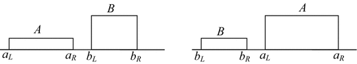

Type-1 intervals

Case 2:

These two intervals are partially related or overlapping (see Fig. 3).

Fig. 3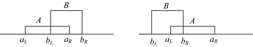

Type-2 intervals

Case 3:

Any one of the intervals contains other (see Fig. 4).

Fig. 4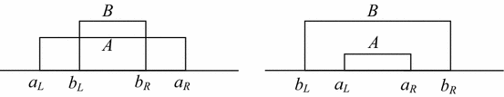

Type-3 intervals

Sahoo et al. [65] have proposed the definitions of interval order relations between two interval numbers in order to solve the maximization and minimization problems.

Definition 3

Order relation of type $>_{\hbox{max} }$ between two intervals. Let us consider two intervals $A = [a_{\text{L}} ,a_{\text{R}} ] = \left\langle {a_{\text{c}} ,a_{\text{w}} } \right\rangle$ and $B = [b_{\text{L}} ,b_{\text{R}} ] = \left\langle {b_{\text{c}} ,b_{\text{w}} } \right\rangle$. Therefore, for solving the maximization problems, the following properties hold:

• 1. $A >_{\hbox{max} } B \Leftrightarrow a_{\text{c}} > b_{\text{c}} \;{\text{for}}\;{\text{Type}}\;{\text{I}}\;{\text{and}}\;{\text{Type}}\;{\text{II}}\;{\text{intervals}},$

• 2. $A >_{\hbox{max} } B \Leftrightarrow$ either $a_{\text{c}} \ge b_{\text{c}} \wedge a_{\text{w}} < b_{\text{w}}$ or $a_{\text{c}} \ge b_{\text{c}} \wedge a_{\text{R}} > b_{\text{R}} \;{\text{for}}\;{\text{Type}}\;{\text{III}}\;{\text{intervals}},$

According to the above definition, the interval number $A$ is accepted for maximization case. So, the order relation $A >_{\hbox{max}} B$ is not symmetric, but it is reflexive and transitive.

Definition 4

Order relation of type $<_{\hbox{min} }$ between two intervals. Let us consider two interval numbers $A = [a_{\text{L}} ,a_{\text{R}} ] = \left\langle {a_{\text{c}} ,a_{\text{w}} } \right\rangle$ and $B = [b_{\text{L}} ,b_{\text{R}} ] = \left\langle {b_{\text{c}} ,b_{\text{w}} } \right\rangle$. Then, for solving the minimization problems, the following properties hold:

• 1. $A <_{\hbox{min} } \; B \Leftrightarrow a_{\text{c}} < b_{\text{c}} \;{\text{for}}\;{\text{Type}}\;{\text{I}}\;{\text{and}}\;{\text{Type}}\;{\text{II}}\;{\text{intervals}},$

• 2. $A <_{\hbox{min} } \; B \Leftrightarrow$ either $a_{\text{c}} \le b_{\text{c}} \wedge a_{\text{w}} < b_{\text{w}}$ or $a_{\text{c}} \le b_{\text{c}} \wedge a_{\text{L}} < b_{\text{L}} \;{\text{for}}\;{\text{Type}}\;{\text{III}}\;{\text{intervals}},$

According to the above definition, the interval $A$ is accepted for minimization case. So, the order relation $A \,{<_{\hbox{min} }}\, B$ is reflexive and transitive, but it is not symmetric.

$A \,{<_{\hbox{min} }}\, B$ is reflexive and transitive, but it is not symmetric.

References

Harris, F.W.: How many parts to make at once, factory. Mag. Manag. 10(2), 135–136 and 152 (1913)
Ghare, P.M., Schrader, G.F.: A model for exponentially decaying inventory. J. Ind. Eng. 14(5), 238–243 (1963)
Chen, S.C., Cárdenas-Barrón, L.E., Teng, J.T.: Retailer’s economic order quantity when the supplier offers conditionally permissible delay in payments link to order quantity. Int. J. Prod. Econ. 155, 284–291 (2014)
Haley, C.W., Higgins, R.C.: Inventory policy and trade credit financing. Manag. Sci. 20(4-part-i), 464–471 (1973)
Goyal, S.K.: Economic order quantity under conditions of permissible delay in payments. J. Oper. Res. Soc. 36(4), 335–338 (1985)
Aggarwal, S.P., Jaggi, C.K.: Ordering policies of deteriorating items under permissible delay in payments. J. Oper. Res. Soc. 46(5), 658–662 (1995)
Jamal, A.M.M., Sarker, B.R., Wang, S.: An ordering policy for deteriorating items with allowable shortages and permissible delay in payment. J. Oper. Res. Soc. 48(8), 826–833 (1997)
Emmons, H.: A replenishment model for radioactive nuclide generators. Manag. Sci. 14(5), 263–274 (1968)
Covert, R.P., Philip, G.C.: An EOQ model for items with Weibull distribution deterioration. AIIE Trans. 5(4), 323–326 (1973)
Giri, B.C., Jalan, A.K., Chaudhuri, K.S.: Economic order quantity model with Weibull deterioration distribution, shortage and ramp-type demand. Int. J. Syst. Sci. 34(4), 237–243 (2003)
Ghosh, S.K., Chaudhuri, K.S.: An order-level inventory model for a deteriorating item with Weibull distribution deterioration, time-quadratic demand and shortages. Adv. Model. Optim. 6(1), 21–35 (2004)
Chakrabarty, T., Giri, B.C., Chaudhuri, K.S.: An EOQ model for items with Weibull distribution deterioration, shortages and trended demand: an extension of Philip’s model. Comput. Oper. Res. 25(7), 649–657 (1998)
Giri, B.C., Chakraborty, T., Chaudhuri, K.S.: Retailer’s optimal policy for perishable product with shortages when supplier offers all-unit quantity and freight cost discounts. Proc. Natl. Acad. Sci. 69(A), 315–326 (1999)
Sana, S., Goyal, S.K., Chaudhuri, K.S.: A production–inventory model for a deteriorating item with trended demand and shortages. Eur. J. Oper. Res. 157(2), 357–371 (2004)
Sana, S., Chaudhuri, K.S.: On a volume flexible production policy for deteriorating item with stock-dependent demand rate. Nonlinear Phenom. Complex Syst. 7(1), 61–68 (2004)
Misra, R.B.: Optimum production lot-size model for a system with deteriorating inventory. Int. J. Prod. Res. 13(5), 495–505 (1975)
Deb, M., Chaudhuri, K.S.: An EOQ model for items with finite rate of production and variable rate of deterioration. Opsearch 23, 175–181 (1986)
Giri, B.C., Pal, S., Goswami, A., Chaudhuri, K.S.: An inventory model for deteriorating items with stock-dependent demand rate. Eur. J. Oper. Res. 95(3), 604–610 (1996)
Goswami, A., Chaudhuri, K.S.: An EOQ model for deteriorating items with shortage and a linear trend in demand. J. Oper. Res. Soc. 42(12), 1105–1110 (1991)
Bhunia, A.K., Maiti, M.: Deterministic inventory model for deteriorating items with finite rate of replenishment dependent on inventory level. Comput. Oper. Res. 25(11), 997–1006 (1998)
Bhunia, A.K., Maiti, M.: An inventory model of deteriorating items with lot-size dependent replenishment cost and a linear trend in demand. Appl. Math. Model. 23(4), 301–308 (1999)
Mandal, B.N., Phaujdar, S.: An inventory model for deteriorating items and stock-dependent consumption rate. J. Oper. Res. Soc. 40(5), 483–488 (1989)
Padmanabhan, G., Vrat, P.: EOQ models for perishable items under stock-dependent selling rate. Eur. J. Oper. Res. 86(2), 281–292 (1995)
Pal, S., Goswami, A., Chaudhuri, K.S.: A deterministic inventory model for deteriorating items with stock-dependent demand rate. Int. J. Prod. Econ. 32(3), 291–299 (1993)
Mandal, M., Maiti, M.: Inventory model for damageable items with stock-dependent demand and shortages. Opsearch 34(3), 156–166 (1997)
Goyal, S.K., Gunasekaran, A.: An integrated production-inventory-marketing model for deteriorating items. Comput. Ind. Eng. 28(4), 755–762 (1995)
Sarker, B.R., Mukherjee, S., Balan, C.V.: An order-level lot-size inventory model with inventory-level dependent demand and deterioration. Int. J. Prod. Econ. 48(3), 227–236 (1997)
Pal, A.K., Bhunia, A.K., Mukherjee, R.N.: Optimal lot size model for deteriorating items with demand rate dependent on displayed stock level (DSL) and partial backordering. Eur. J. Oper. Res. 175(2), 977–991 (2006)
Raafat, F.: Survey of literature on continuously deteriorating inventory models. J. Oper. Res. Soc. 42(1), 27–37 (1991)
Goyal, S.K., Giri, B.C.: Recent trends in modeling of deteriorating inventory. Eur. J. Oper. Res. 134(1), 1–16 (2001)
Bakker, M., Riezebos, J., Teunter, R.H.: Review of inventory systems with deterioration since 2001. Eur. J. Oper. Res. 221(2), 275–284 (2012)
Janssen, L., Claus, T., Sauer, J.: Literature review of deteriorating inventory models by key topics from 2012 to 2015. Int. J. Prod. Econ. 182, 86–112 (2016)
Summers, B., Wilson, N.: An empirical investigation of trade credit demand. Int. J. Econ. Bus. 9(2), 257–270 (2002)
Seifert, D., Seifert, R.W., Protopappa-Sieke, M.: A review of trade credit literature: opportunities for research in operations. Eur. J. Oper. Res. 231(2), 245–256 (2013)
Teng, J.T.: On the economic order quantity under conditions of permissible delay in payments. J. Oper. Res. Soc. 53(8), 915–918 (2002)
Das, B.C., Das, B., Mondal, S.K.: An integrated production inventory model under interactive fuzzy credit period for deteriorating item with several markets. Appl. Soft Comput. 28, 453–465 (2015)
Das, B.C., Das, B., Mondal, S.K.: An integrated production-inventory model with defective item dependent stochastic credit period. Comput. Ind. Eng. 110, 255–263 (2017)
Guchhait, P., Maiti, M.K., Maiti, M.: A production inventory model with fuzzy production and demand using fuzzy differential equation: an interval compared genetic algorithm approach. Eng. Appl. Artif. Intell. 26(2), 766–778 (2013)
Guchhait, P., Maiti, M.K., Maiti, M.: Inventory model of a deteriorating item with price and credit linked fuzzy demand: a fuzzy differential equation approach. Opsearch 51(3), 321–353 (2014)
Chang, C.T., Ouyang, L.Y., Teng, J.T.: An EOQ model for deteriorating items under supplier credits linked to ordering quantity. Appl. Math. Model. 27(12), 983–996 (2003)
Abad, P.L., Jaggi, C.K.: A joint approach for setting unit price and the length of the credit period for a seller when end demand is price sensitive. Int. J. Prod. Econ. 83(2), 115–122 (2003)
Ouyang, L.Y., Wu, K.S., Yang, C.T.: A study on an inventory model for non-instantaneous deteriorating items with permissible delay in payments. Comput. Ind. Eng. 51(4), 637–651 (2006)
Huang, Y.F.: An inventory model under two levels of trade credit and limited storage space derived without derivatives. Appl. Math. Model. 30(5), 418–436 (2006)
Huang, Y.F.: Economic order quantity under conditionally permissible delay in payments. Eur. J. Oper. Res. 176(2), 911–924 (2007)
Huang, Y.F.: Optimal retailer’s replenishment decisions in the EPQ model under two levels of trade credit policy. Eur. J. Oper. Res. 176(3), 1577–1591 (2007)
Sana, S.S., Chaudhuri, K.S.: A deterministic EOQ model with delays in payments and price-discount offers. Eur. J. Oper. Res. 184(2), 509–533 (2008)
Huang, Y.F., Hsu, K.H.: An EOQ model under retailer partial trade credit policy in supply chain. Int. J. Prod. Econ. 112(2), 655–664 (2008)
Ho, C.H., Ouyang, L.Y., Su, C.H.: Optimal pricing, shipment and payment policy for an integrated supplier–buyer inventory model with two-part trade credit. Eur. J. Oper. Res. 187(2), 496–510 (2008)
Bhunia, A.K., Shaikh, A.A., Sahoo, L.: A two-warehouse inventory model for deteriorating items under permissible delay in payment via particle swarm optimization. Int. J. Logist. Syst. Manag. 24(1), 45–68 (2016)
Jaggi, C.K., Tiwari, S., Shafi, A.: Effect of deterioration on two-warehouse inventory model with imperfect quality. Comput. Ind. Eng. 88, 378–385 (2015)
Jaggi, C., Sharma, A., Tiwari, S.: Credit financing in economic ordering policies for non-instantaneous deteriorating items with price dependent demand under permissible delay in payments: a new approach. Int. J. Ind. Eng. Comput. 6(4), 481–502 (2015)
Jaggi, C.K., Tiwari, S., Goel, S.K.: Credit financing in economic ordering policies for non-instantaneous deteriorating items with price dependent demand and two storage facilities. Ann. Oper. Res. 248(1–2), 253–280 (2017)
Tiwari, S., Cárdenas-Barrón, L.E., Khanna, A., Jaggi, C.K.: Impact of trade credit and inflation on retailer’s ordering policies for non-instantaneous deteriorating items in a two-warehouse environment. Int. J. Prod. Econ. 176, 154–169 (2016)
Jaggi, C.K., Yadavalli, V.S.S., Sharma, A., Tiwari, S.: A fuzzy EOQ model with allowable shortage under different trade credit terms. Appl. Math. Inf. Sci. 10(2), 785–805 (2016)
Jaggi, C., Tiwari, S., Goel, S.: Replenishment policy for non-instantaneous deteriorating items in a two storage facilities under inflationary conditions. Int. J. Ind. Eng. Comput. 7(3), 489–506 (2016)
Bhunia, A.K., Mahato, S.K., Shaikh, A.A., Jaggi, C.K.: A deteriorating inventory model with displayed stock-level-dependent demand and partially backlogged shortages with all unit discount facilities via particle swarm optimisation. Int. J. Syst. Sci. Oper. Logist. 1(3), 164–180 (2014)
Bhunia, A.K., Shaikh, A.A.: Investigation of two-warehouse inventory problems in interval environment under inflation via particle swarm optimization. Math. Comput. Model. Dyn. Syst. 22(2), 160–179 (2016)
Grzegorzewski, P.: Nearest interval approximation of a fuzzy number. Fuzzy Sets Syst. 130(3), 321–330 (2002)
Bhunia, A.K., Shaikh, A.A.: An application of PSO in a two-warehouse inventory model for deteriorating item under permissible delay in payment with different inventory policies. Appl. Math. Comput. 256, 831–850 (2015)
Kennedy, J.F., Eberhart, R.C.: Particle swarm optimization. In: Proceedings of the IEEE International Conference on Neural Network, vol. IV, Perth, Australia, pp. 1942–1948 (1995)
Clerc, M., Kennedy, J.: The particle swarm-explosion, stability, and convergence in a multidimensional complex space. IEEE Trans. Evol. Comput. 6(1), 58–73 (2002)
Clerc, M.: The swarm and the queen: towards a deterministic and adaptive particle swarm optimization: In: Proceedings of the 1999 Congress on Evolutionary Computation, 1999, CEC 99, vol. 3, pp. 1951–1957. IEEE (1999)
Sun, J., Feng, B., Xu, W.: Particle swarm optimization with particles having quantum behaviour. In: Congress on Evolutionary Computation, 2004, CEC2004, vol. 1, pp. 325–331. IEEE (2004)
Sun, J., Xu, W., Feng, B.: A global search strategy of quantum-behaved particle swarm optimization. In: 2004 IEEE Conference on Cybernetics and Intelligent Systems, vol. 1, pp. 111–116. IEEE (2004)
Sahoo, L., Bhunia, A.K., Kapur, P.K.: Genetic algorithm based multi-objective reliability optimization in interval environment. Comput. Ind. Eng. 62(1), 152–160 (2012)
Acknowledgements
We thank the editor and anonymous reviewers for their constructive feedback on earlier drafts of this manuscript. The Tecnológico de Monterrey Research Group in Industrial Engineering and Numerical Methods 0822B01006 supported the first and third authors.
Author information
Authors and Affiliations
Corresponding author