Flexural Performance of Steel–FRP Composites for Automotive Applications

Abstract

The design of hybrid structure offers an attractive solution to enhance strength and structural stiffness as well as to achieve lightweight effect and cost reduction. The applications of steel–FRP (fiber-reinforced polymer) composites in transportation and civil engineering have been comprehensively reviewed. In order to apply hybrid structures to car body parts such as B-pillar, flexural performance of steel–FRP composites is investigated by means of three-point bending test in this study. An analytical model is deduced to calculate the initial stiffness, the bending load and the energy absorption of steel–FRP composites. Steel–CFRP (carbon fiber-reinforced polymer) and steel–AFRP (aramid fiber-reinforced polymer) composites are experimentally studied and discussed. The results demonstrate that the steel–FRP composites exhibit significantly higher load-carrying capabilities and initial stiffnesses along with larger energy absorptions in the bending process compared to the single steel sheet.

1 Introduction

Lightweight design has attracted increasing attention in automotive industry owing to the demand of reducing CO₂ emissions [1]. Developing lightweight materials is one of the main research directions in the area of automotive lightweight [2]. Lightweight can be achieved by using a single material with high performance (e.g., high strength) or by combining dissimilar materials to form a composite or hybrid structure [3]. Applying high-strength materials offers an opportunity to reduce weight through decreasing wall thickness of a structure; however, excessive wall thickness reduction may lead to instability of a structure due to insufficient stiffness. The application of pure composite material (e.g., carbon fiber-reinforced polymers, CFRP) has disadvantages like high cost and long cycle time in production. Hence, it came up with the idea of employing two materials to form a hybrid structure utilizing the respective advantages and complementing each other. This idea matches well with the lightweight design concept of “the right material applied on right place” [4, 5]. Optimal design of a hybrid structure gives full play to the respective constituents in strength, stiffness and weight reduction and allows to balance cost and weight of the hybrid structure [6,7,8]. Metal–FRP hybrid structures are fabricated from metal and fiber-reinforced polymer (FRP), where metal and FRP are adhesively bonded. Metal serves as the base of the structural component, and FRP offers the possibility to enhance the mechanical properties of the structure such as load-carrying capability and stiffness due to the high specific strength and specific stiffness of fibers, e.g., carbon fibers, aramid fibers, etc. In addition, the mechanical properties of metal–FRP composites vary with the types of fiber and matrix as well as fiber orientation; therefore, metal material (i.e., material with good toughness and impact resistance) overcomes drawbacks of FRP (e.g., low ductility and poor impact resistance), and the combination of metal and FRP generates outstanding overall mechanical performance [9].

The earliest application of metal–FRP composites traces back to the 1970s. The aerospace industry introduced a new hybrid material, i.e., aramid fiber-reinforced aluminum laminate as illustrated in Fig. 1, which combines superior impact resistance of aluminum alloy and fatigue resistance of aramid fiber-reinforced polymers (AFRP) to improve the resistance of crack propagation of the hybrid structure [4]. At present, metal–FRP composites, e.g., from aluminum alloy and glass fiber-reinforced polymers (GFRP), are widely applied on the airbus A380 airplane [10].

Fig. 1

Aramid fiber-reinforced aluminum laminate [4]

In the 1990s, the application of FRP gradually spread to the field of civil engineering, where FRP acted as a reinforcement of concrete and/or steel structures to meet specific requirements of structural strength and corrosion resistance. FRP has been used for repair and maintenance of concrete beams against seismic action after the Kobe earthquake in 1995 [11], and since then, FRP has been paid much attention by the engineering community. CFRP has been widely used in this field, and it is generally adhered onto the surface of a steel structure by adhesives (e.g., epoxy resin) for load-sharing, as shown in Fig. 2. It was found that the reinforcement of CFRP contributed greatly to increasing load-carrying ability of an undamaged structure or to preventing crack initiation and propagation in a damaged structure [12,13,14,15]. In addition, reinforcement by CFRP exhibits advantages of high corrosion resistance with nearly negligible weight increase in comparison with other reinforcing approaches (e.g., externally bonding steel sheet to concrete structures).

Fig. 2

An application of CFRP reinforcement on civil structures [14]

Since 2010, metal–FRP hybrid structures have been gradually applied in automotive industry, and they are mainly utilized to improve energy absorptions, NVH performances and load-carrying abilities of car body components. Figure 3 presents an Al–GFRP hybrid front bumper from the Benteler, where GFRP was used to enhance the crashworthiness of the aluminum alloy front bumper. It was reported that the Al–GFRP hybrid structure succeeded in increasing the energy absorption in a collision test and reducing 45% weight compared with a steel–aluminum component [15]. Figure 4 presents an aluminum subframe reinforced by Hexcel’s fast-curing carbon fiber prepreg [16]. The testing result indicated that the hybrid subframe demonstrated a positive effect on improving overall NVH performance through adhering merely 500 g CFRP prepreg, and its total weight was significantly reduced in comparison with the all-metal ones.

Fig. 3

An Al–GFRP hybrid front bumper [15]

Fig. 4

An Al–CFRP hybrid subframe [16]

Passive safety is a key issue in automotive industry [17]. The safety components such as A-pillar assembly and B-pillar assembly play a vital role in ensuring vehicle safety to resist bending during a side crash, and locally reinforcing safety structures is a common approach to improve their stiffnesses and load-carrying abilities to achieve excellent crash performances [1, 18]. Figure 5 presents a hybrid A-pillar assembly from a soft top convertible, which was applied to Porsche 911 series [19]. The A-pillar assembly is fabricated from several elements, i.e., glass fibers and high-strength steel, and all elements are bonded with adhesive. The hybrid A-pillar assembly exhibits similar crashworthiness, but is around 5 kg lighter compared to the all-steel A-pillar assembly.

Fig. 5

A steel–GFRP hybrid A-pillar assembly from Porsche [19]

In 2015, BMW 7 series firstly strengthened B-pillar assembly by rivet-bonding with a preformed CFRP reinforcement, as shown in Fig. 6, which achieved an improvement in crashworthiness of car body as well as a weight reduction [6, 20]. Lee et al. [21] compared the collision testing results of B-pillars fabricated from tailor-welded steel blanks and steel–CFRP hybrid structures. The result shows that the weight of the hybrid structure was reduced by 44%, while its crashworthiness was improved by 10% compared with that of the tailor-welded steel B-pillar.

Fig. 6

A steel–CFRP hybrid B-pillar assembly from BMW [20]

Metal–FRP hybrid structures are complex multi-components and multi-interface systems. It has been reported that the mechanical properties and deformation behavior of a hybrid structure are affected by mechanical properties of FRP and metal, interfacial properties between metal and FRP, fiber orientation and direction of applied load [22]. Finite element method is commonly employed to investigate the mechanical behavior of a metal–FRP hybrid structure, especially to predict progressive failure during deformation. Jin et al. [23] established a 3D constitutive model to predict the ductile damage of aluminum, failure of GFRP and interface delamination of Al–GFRP composites during three-point bending, as shown in Fig. 7a. Dhaliwal et al. [24] modeled the progressive damage behavior of Al–CFRP composites under static flexural loading and found that the progressive damage behavior of a multilayer Al–CFRP composite was affected by the position of carbon fiber–epoxy layers in the composite. Xu et al. [25] developed a numerical model of an Al–CFRP composite under an in-plane bending condition; the simulation results suggested that the primary damage modes were the yielding of aluminum in the midspan and delamination between the aluminum and CFRP layers. The effect of metal volume fraction on the failure modes of Al–CFRP hybrid beams was investigated by Dhaliwal and Newaz [26] using FE simulation with FE model shown in Fig. 7b. It was found that the failure mode changed from rupture in the midspan of the hybrid beam to gradual deformation with an increase in the metal volume fraction in an Al–CFRP hybrid beam. There are some studies analyzing mechanical behavior of a metal–FRP hybrid structure in terms of initial stiffness, bending load versus displacement and energy absorption during three-point bending or axial crushing [27,28,29]. The aforementioned studies suggest that finite element simulation is a vital tool to predict deformation behavior of steel–FRP hybrid structures. However, it is still difficult to understand and clearly clarify the strengthening mechanism of metal–FRP hybrid structures simply by using finite element simulation. Nevertheless, analytical models are of significance to describe and analyze such mechanism.

Fig. 7

Finite element models of a an Al–GFRP composite [23] and b an Al–CFRP hybrid beam [26] during three-point bending

The existing theoretical studies in literature focus primarily on the prediction of interfacial stresses in a metal–FRP composite to avoid debonding during deformation. Ghafoori et al. [30] conducted an analytical study to predict interfacial shear stresses of simply supported steel beams strengthened through bonding prestressed or non-stressed FRP plates, and the distributions of interfacial shear stresses between steel and FRP under typical boundary conditions were given. It is also found in Ref. [30] that prestressing FRP did not affect the stiffness of a plated beam, but helped to increase its yield and maximum bending loads. Mohamed et al. [31] proposed a theoretical model of interfacial stress distribution of FRP reinforced concrete beams under bending loads accounting for creep and shrinkage effects. Based on the deformation compatibility approach, Guenaneche et al. [32] presented a theoretical analysis method to solve interface stresses of simply supported concrete–FRP hybrid beams subjected to arbitrary loading and concluded that shear stresses were distributed in a parabolic manner through the thickness of the adhesive layer. However, there are very limited studies reporting the mechanical performances of metal–FRP composites and/or hybrid structures, and the associated analytical models were developed mostly under tensile conditions [33, 34] or axial crushing conditions [35, 36]. In addition, the current models are only capable of predicting the mechanical performances of the hybrid structure under elastic deformation, and it is required to take into account nonlinear mechanical properties of metals (e.g., plastic deformation) [37] in fundamental research.

According to Lin et al. [38], steel–FRP composites behave differently from bending to compression and to tension. It should also be noted that bending is a typical deformation mode of vehicle safety structures during crashes, e.g., A/B-pillar assemblies in a side crash and front bumpers in a front crash. A theoretical model was developed by Kecman [39] to describe the bending collapse behavior of thin-walled structures. As exemplarily illustrated in Fig. 8, the bending process of a thin-walled structure can be considered as a combination of two deformation modes, i.e., flexural deformation of the top and bottom thin sheets, and compressive deformation of the two side walls. Therefore, studying the flexural performances of steel–FRP composites is crucial to systematically understand the deformation behavior and strengthening mechanism of steel–FRP hybrid structures during which the analytical approach employed plays an essential role in the application of FRP reinforcement to automotive bodies.

Fig. 8

The flexural deformation can be regarded as a combination of the flexural deformation of flat sheets on the top and bottom, and the compressive deformation of the side walls

In this work, the flexural performance of steel–FRP composites was studied by means of three-point bending. An analytical model, which accounts for plastic deformation of the steel, has been deduced to calculate the bending moments and bending loads of the steel–FRP composites. Three-point bending tests of steel–FRP hybrid sheets were carried out to validate the analytical model. The reinforcing effect of FRP on bending moment and energy absorption of steel–FRP composites were discussed on the basis of the analytical model.

2 Analytical Modeling

An analytical model of three-point bending has been developed in this study to investigate the flexural behaviors of steel–FRP composites. The following assumptions in the analytical modeling are listed in details:

• 1. The steel–FRP composite is placed on two supports in a three-point bending test with no external forces applied along the tangential direction.

• 2. The steel–FRP composite always keeps line contact with the supports along the length of the support, which is parallel to the supports’ axis during bending process.

• 3. The widths of two constituents ($b_{\text{s}}$ and $b_{\text{FRP}}$) are large enough compared to their thicknesses. Therefore, the strain of the composite is zero in the width direction [40].

• 4. The thicknesses of two constituents ($t_{\text{s}}$ and $t_{\text{FRP}}$) remain constant during and after the bending.

• 5. No relative sliding between the contact point of the steel–FRP composite and the support (i.e., points A₁ and B₁ in Fig. 9 in the x–y plane) occurs under three-point bending, and the elastic deformation of the composite in a three-point bending test is small due to the low elongation of FRP. Thus, the length of steel–FRP composite between points A₁ and B₁ is assumed to be constant in a three-point bending test.

  Fig. 9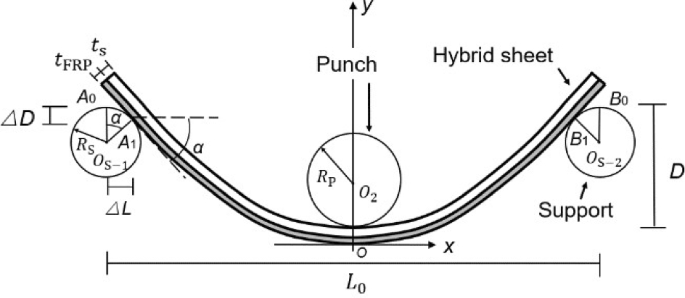

  

  Geometries of the steel–FRP composite, the support and the punch arrangement in a three-point bending test

• 6. Only after the fracture of fibers, debonding between FRP and steel occurs during bending process.

• 7. Maximum bending load can be achieved as carbon fibers or aramid fibers reach the fracture strain [41].

2.1 Calculation of Bending Radius

Figure 9 shows the schematic of steel–FRP composite, support and punch in a three-point bending test. The punch is in contact with the composite at the midspan and is given the displacement D. The composite is in contact with the supports at points A and B in the x–y plane, the coordinates of which are $\left( {x_{A} ,y_{A} } \right)$ and $\left( {x_{B} ,y_{B} } \right)$, respectively. The subscripts 0 and 1 of points A and B denote the points at the beginning of bending process and at a certain moment during bending, respectively. The curve A₁B₁ is tangent to the two cylindrical supports, respectively, at points A₁ and B₁. According to the study of Tolomeo [42], the deformed shape of the steel–metal composite can be simplified to an on-axis parabola, which can be expressed by

$$ y\left( x \right) = \frac{{x^{2} }}{2p} $$

(1)

where p (p > 0) is a parameter determining a parabola. The slopes of the tangent lines of y(x) at points A and B (e.g., $k_{A}$ and $k_{B}$) are given by Eq. (2).

$$ \begin{array}{*{20}l} {k_{\text{A}} = \frac{{x_{\text{A}} }}{p} = \tan \alpha } \hfill \\ {k_{\text{B}} = \frac{{x_{\text{B}} }}{p} = - \tan \alpha } \hfill \\ \end{array} $$

(2)

where $\alpha$ is the deflection angle between the tangent line of y(x) at point A and the x-axis. Based on assumption (5), the length of steel–FRP composite between points A₁ and B₁ remains a constant value of $L_{0}$ (namely the initial span length), which can be expressed as

$$ L_{0} = \frac{{x_{\text{A}1} }}{p}\sqrt {x_{\text{A}1}^{2} + p^{2} } + p\ln \left( {x_{\text{A}1} + \sqrt {x_{\text{A}1}^{2} + p^{2} } } \right) - p\ln p $$

(3)

By substituting Eq. (2) into Eq. (3), the value of p during bending (with a given value of $\alpha$) can be calculated as

$$ p = \frac{{L_{0} }}{{\tan \alpha \sqrt {\tan^{2} \alpha + 1} + \ln \left( {\tan \alpha + \sqrt {\tan^{2} \alpha + 1} } \right)}} $$

(4)

Thus, the punch displacement D can be calculated:

$$ D = \frac{{x_{\text{A}}^{2} }}{2p} + \Delta D = \frac{{p \cdot \tan^{2} \alpha }}{2} + R_{\text{S}} \cdot (1 - \cos \alpha ) $$

(5)

where $\Delta D$ is the displacement in the y direction due to the rotation of the support. $R_{\text{S}}$ is the radius of the support. The bending radius of the convex surface at the midspan $R_{\text{o}}$ can be expressed by

$$ R_{\text{o}} = \frac{{\left[ {1 + y^{{\prime }} \left( x \right)} \right]^{{\frac{3}{2}}} }}{{y^{{\prime \prime }} \left( x \right)}}|_{x = 0} = p $$

(6)

The bending radius of the concave surface $R_{\text{i}}$ and the neutral layer $R_{\text{n}}$ can be expressed by Eqs. (7) and (8), respectively.

$$ R_{\text{i}} = R_{\text{o}} - t_{\text{s}} - t_{\text{FRP}} $$

(7)

$$ R_{\text{n}} = R_{\text{i}} + y_{\text{n}} $$

(8)

where $y_{\text{n}}$ denotes the distance between the concave surface and the neutral layer and will be discussed in Sect. 2.3.

2.2 Stress and Strain Calculations

According to Refs. [43,44,45] and assumption (1), the tangential and transverse strains through sheet thickness can be obtained.

$$ \varepsilon_{\text{r}} + \varepsilon_{\uptheta } = 0 $$

(9)

$$ \varepsilon_{\uptheta } = \ln \frac{r}{{R_{\text{n}} }} $$

(10)

where $\varepsilon_{\uptheta }$ and $\varepsilon_{\text{r}}$ are the tangential and transverse strains, respectively, and r is the radius of the concerned bending layer. The nonlinear strain-hardening behavior of steel is considered in this model. The distribution of the tangential stress $\sigma_{\uptheta }$ through sheet thickness can be expressed as Eq. (11) on the basis of stress–strain relationship [40] and Hill48 quadratic yield function [46].

$$ \sigma_{\theta } = \left\{ {\begin{array}{*{20}l} { - fk\left( {\varepsilon_{0} - f\ln \frac{r}{{R_{\text{n}} }}} \right)^{n} ,\quad R_{\text{i}} \le r \le R_{\text{n}} - C} \\ {\frac{{E_{\text{s}} }}{{1 - \gamma_{\text{s}}^{2} }}\ln \frac{r}{{R_{\text{n}} }} = E_{\text{s}}^{'} \ln \frac{r}{{R_{\text{n}} }},\quad R_{\text{n}} - C \le r \le R_{\text{n}} + C} \\ {fk\left( {\varepsilon_{0} + f\ln \frac{r}{{R_{\text{n}} }}} \right)^{n} ,\quad R_{\text{n}} + C \le r \le R_{\text{o}} - t_{\text{FRP}} } \\ \end{array} } \right. $$

(11)

where $E_{\text{s}}$ and $E_{\text{s}}^{'}$ are the elastic modulus of steel in uniaxial tensile and plane strain conditions, respectively [47], f is a parameter related to the transverse anisotropy in plane strain condition, which equals to $\left( {1 + \bar{r}} \right)/\sqrt {1 + 2\bar{r}}$, and $\bar{r}$ is the transverse anisotropy coefficient. For simplicity, $\bar{r}$ of the investigated steel is selected as 1 and f is then calculated as $2/\sqrt 3$ [48], k and n denote the hardening exponent and the strength coefficient, respectively. C is the half thickness of elastic region (i.e., as shown in Fig. 10), which can be defined as

$$ C = \frac{{\sigma_{\text{s}}^{\text{S}} R_{\text{n}} \left( {1 - \gamma_{\text{s}}^{2} } \right)}}{{E_{\text{s}} }} $$

(12)

where $\sigma_{\text{s}}^{\text{S}}$ and $\gamma_{\text{s}}$ denote the yield strength and the Poisson’s ratio of steel, respectively.

Fig. 10

Elastic and plastic regions of the steel–FRP composite under three-point bending

The FRP composite material is described as a linear elastic material in this study, and its stress–strain relationship can be expressed by the following equation:

$$ \sigma_{\text{FRP}} = \left\{ {\begin{array}{*{20}l} {E_{\text{FRP}}^{1} \varepsilon_{\text{FRP}} , 0 \le \varepsilon_{\text{FRP}} \le \varepsilon_{\text{FRP}}^{\text{U}} } \\ {0, \varepsilon_{\text{FRP}} > \varepsilon_{\text{FRP}}^{\text{U}} } \\ \end{array} } \right. $$

(13)

where $E_{\text{FRP}}^{1}$ denotes the elastic modulus of FRP along fiber direction. $\varepsilon_{\text{FRP}}$ and $\varepsilon_{\text{FRP}}^{\text{U}}$ are the true strain and the fracture strain of FRP, respectively. When the true strain of FRP is beyond $\varepsilon_{\text{FRP}}^{\text{U}}$, the steel–FRP composite is regarded to have the same bendability with a single steel sheet. The elastic modulus of FRP along fiber direction $E_{\text{FRP}}^{1}$ can be calculated by Eq. (14) [49]. According to Ref. [50], the elastic modulus of FRP in plane strain condition can be calculated by Eq. (15).

$$ E_{\text{FRP}}^{1} = V_{\text{f}} E_{\text{f}} + \left( {1 - V_{\text{f}} } \right)E_{\text{m}} $$

(14)

$$ E_{\text{FRP}}^{'} = \frac{{E_{\text{FRP}}^{1} }}{{1 - \nu_{\text{FRP}}^{12} \nu_{\text{FRP}}^{21} }} $$

(15)

where $E_{\text{f}}$ and $E_{\text{m}}$ denote the elastic modulus of fiber along fiber direction and the elastic modulus of matrix, respectively. $V_{\text{f}}$ is the fiber volume. $\nu_{\text{FRP}}^{12}$ and $\nu_{\text{FRP}}^{21}$ are the major and minor Poisson’s ratio of FRP, respectively.

$$ \mathop \smallint \limits_{{R_{\text{n}} }}^{{R_{\text{n}} + t_{\text{s}} - y_{\text{n}} }} E_{\text{s}}^{'} \ln \frac{r}{{R_{\text{n}} }}b_{\text{s}} {\text{d}}r + \mathop \smallint \limits_{{R_{\text{n}} + t_{\text{s}} - y_{\text{n}} }}^{{R_{\text{n}} + t_{\text{s}} + t_{\text{FRP}} - y_{\text{n}} }} E_{\text{FRP}}^{'} \ln \frac{r}{{R_{\text{n}} }}b_{\text{FRP}} {\text{d}}r - \mathop \smallint \limits_{{R_{\text{n}} - y_{\text{n}} }}^{{R_{\text{n}} }} E_{\text{s}}^{'} \ln \frac{r}{{R_{\text{n}} }}b_{\text{s}} {\text{d}}r = 0 $$

(16)

$$ \mathop \smallint \limits_{{R_{\text{n}} }}^{{R_{\text{n}} + C}} E_{\text{s}}^{'} \ln \frac{r}{{R_{\text{n}} }}b_{\text{s}} {\text{d}}r + \mathop \smallint \limits_{{R_{\text{n}} + C}}^{{R_{\text{n}} + t_{\text{s}} - y_{\text{n}} }} fk\left( {\varepsilon_{0} + f\ln \frac{r}{{R_{\text{n}} }}} \right)^{n} b_{\text{s}} {\text{d}}r + \mathop \smallint \limits_{{R_{\text{n}} + t_{\text{s}} - y_{\text{n}} }}^{{R_{\text{n}} + t_{\text{s}} + t_{\text{FRP}} - y_{\text{n}} }} E_{\text{FRP}}^{'} \ln \frac{r}{{R_{\text{n}} }}b_{\text{FRP}} {\text{d}}r - \mathop \smallint \limits_{{R_{\text{n}} - C}}^{{R_{\text{n}} }} E_{\text{s}}^{'} \ln \frac{r}{{R_{\text{n}} }}b_{\text{s}} {\text{d}}r - \mathop \smallint \limits_{{R_{\text{n}} - y_{\text{n}} }}^{{R_{\text{n}} - C}} fk\left( {\varepsilon_{0} - f\ln \frac{r}{{R_{\text{n}} }}} \right)^{n} b_{\text{s}} {\text{d}}r = 0 $$

(17)

2.3 Modeling of Internal Bending Moment and Bending Load

The geometries, the strain distribution and the tangential stress distribution of the steel–FRP composite through thickness are presented in Fig. 11, where $y_{\text{s}}$ and $y_{\text{FRP}}$ denote the distance between the concave surface of the steel–FRP composite and the middle layer of steel and FRP, respectively, and $\varepsilon_{\text{s}}$ and $\varepsilon_{\text{FRP}}$ denote the true strains of steel and FRP, respectively. $y_{\text{n}}$ can be calculated by Eqs. (16) and (17) when the steel constituent of a steel–FRP composite is under elastic and plastic deformations, respectively. It should be noted that $y_{\text{n}}$ in Fig. 11 is assumed smaller than $t_{\text{s}}$ in this study as $t_{\text{s}}$ is large enough compared with $t_{\text{FRP}}$ and the neutral layer shift is smaller than half of $t_{\text{s}}$; therefore, the thickness of FRP complies with Eq. (18) in this study.

Fig. 11

Geometries, the strain distribution and the tangential stress distribution of the steel–FRP composite through sheet thickness under the conditions of a ${{C}} \ge y_{\text{n}}$, b $t_{\text{s}} - y_{\text{n}} \le {{C}} \le y_{\text{n}}$ and c ${{C}} \le t_{\text{s}} - y_{\text{n}}$

$$ t_{\text{FRP}} < \sqrt {\frac{{b_{\text{s}} E_{\text{s}}^{'} t_{\text{s}}^{2} }}{{b_{\text{FRP}} E_{\text{FRP}}^{'} }}} $$

(18)

Figure 11 shows that steel–FRP composite has a non-uniform tangential stress distribution through thickness due to the different stress–strain relations of two constituents and the neutral layer shift. The evolutions of the elastic and plastic regions through sheet thickness are illustrated in Fig. 11 as well, where the cross-sectional areas hatched with gray color and dots represent the regions under elastic and plastic bending moments, respectively. With an increase in D, the shift of neutral layer increases and the area of steel under elastic deformation decreases in three-point bending. Thus, the bending moments in different stages of bending process need separate discussions.

The internal bending moment of the steel–FRP composite consists of the elastic moments of both steel and FRP when C is larger than $y_{\text{n}}$ (as shown in Fig. 11a), which is expressed by Eq. (19). The internal bending moment of steel–FRP composite consists of the elastic moments of steel and FRP, and the plastic moment of steel when C is shorter than $y_{\text{n}}$. When $t_{\text{s}} - y_{\text{n}} \le {{C}} \le y_{\text{n}}$ (i.e., as presented in Fig. 11b) and $C \le t_{\text{s}} - y_{\text{n}}$ (i.e., as presented in Fig. 11c), the bending moments can be expressed by Eqs. (20) and (21), respectively.

$$ M = M_{{{\text{s}} - {\text{e}}}} + M_{{{\text{FRP}} - {\text{e}}}} = \frac{{\left[ {\left( {t_{\text{s}} - y_{\text{n}} } \right)^{3} + y_{\text{n}}^{3} } \right]b_{\text{s}} E_{\text{s}}^{'} }}{{3R_{\text{n}} }} + \frac{{[\left( {t_{\text{s}} - y_{\text{n}} + t_{\text{FRP}} } \right)^{3} - \left( {t_{\text{s}} - y_{\text{n}} )^{3} } \right]b_{\text{FRP}} E_{\text{FRP}}^{'} }}{{3R_{\text{n}} }} $$

(19)

$$ M = M_{{{\text{s}} - {\text{e}}}} + M_{{{\text{s}} - {\text{p}}}} + M_{{{\text{FRP}} - {\text{e}}}} = \frac{{\left[ {C^{3} + \left( {t_{\text{s}} - y_{\text{n}} } \right)^{3} } \right]b_{\text{s}} E_{\text{s}}^{'} }}{{3R_{\text{n}} }} - \mathop \smallint \limits_{{R_{\text{n}} - y_{\text{n}} }}^{{R_{\text{n}} - {\text{C}}}} fk\left( {\varepsilon_{0} - f\ln \frac{r}{{R_{n} }}} \right)^{n} \left( {r - R_{\text{n}} } \right)b_{\text{s}} {\text{d}}r + \frac{{\left[ {(t_{\text{s}} - y_{\text{n}} + t_{\text{FRP}} )^{3} - \left( {t_{\text{s}} - y_{\text{n}} } \right)^{3} } \right]b_{\text{FRP}} E_{\text{FRP}}^{'} }}{{3R_{\text{n}} }} $$

(20)

$$ \begin{aligned} M & = M_{{{\text{s}} - {\text{e}}}} + M_{{{\text{s}} - {\text{p}}}} + M_{{{\text{FRP}} - {\text{e}}}} = \frac{{2C^{3} b_{\text{s}} E_{\text{s}}^{'} }}{{3R_{\text{n}} }} + \mathop \smallint \limits_{{R_{\text{n}} + C}}^{{R_{\text{n}} + t_{\text{s}} - y_{\text{n}} }} fk\left( {\varepsilon_{0} + f\ln \frac{r}{{R_{\text{n}} }}} \right)^{n} \left( {r - R_{\text{n}} } \right)b_{\text{s}} {\text{d}}r \\ & \quad - \mathop \smallint \limits_{{R_{\text{n}} - y_{\text{n}} }}^{{R_{\text{n}} - C}} fk\left( {\varepsilon_{0} - f\ln \frac{r}{{R_{\text{n}} }}} \right)^{n} \left( {r - R_{\text{n}} } \right)b_{\text{s}} {\text{d}}r + \frac{{[\left( {t_{\text{s}} - y_{\text{n}} + t_{\text{FRP}} } \right)^{3} - \left( {t_{\text{s}} - y_{\text{n}} )^{3} } \right]b_{\text{FRP}} E_{\text{FRP}}^{'} }}{{3R_{\text{n}} }} \\ \end{aligned} $$

(21)

where $M_{{{\text{s}} - {\text{e}}}}$, $M_{{{\text{s}} - {\text{p}}}}$ and $M_{{{\text{FRP}} - {\text{e}}}}$ denote internal bending moments of steel in the elastic and plastic regions (as presented in Fig. 11), and the elastic bending moment of FRP, respectively. According to Chudasama et al. [51], the relationship between the internal bending moment M and bending load $F_{\text{b}}$ in a three-point bending test is given by Eq. (22). By combining with Eqs. (19)–(22), the bending load of a steel–FRP composite in three-point bending can be obtained, i.e., Eq. (23).

$$ M = \frac{{F_{\text{b}} }}{2}\left( {1 - \frac{{L_{0} - R_{\text{S}} \sin \alpha }}{{2L_{0} - R_{\text{S}} \sin \alpha }}} \right)\left( {\frac{1}{\cos \alpha + \mu \sin \alpha }} \right)\left\{ {\frac{{L_{0} }}{2} - \tan \alpha \left( {R_{\text{S}} - D} \right) + \mu \left[ {\frac{{L_{0} }}{2}\tan \alpha - R_{\text{S}} \left( {\frac{{\sin^{2} \alpha }}{\cos \alpha } + \cos \alpha - 1} \right) - D} \right]} \right\} $$

(22)

$$ F_{\text{b}} = \left\{ {\begin{array}{*{20}l} {\frac{{2\left[ {\left( {t_{\text{s}} - y_{\text{n}} } \right)^{3} + y_{\text{n}}^{3} } \right]b_{\text{s}} E_{\text{s}}^{'} + 2[\left( {t_{\text{s}} - y_{\text{n}} + t_{\text{FRP}} } \right)^{3} - \left( {t_{\text{s}} - y_{\text{n}} )^{3} } \right]b_{\text{FRP}} E_{\text{FRP}}^{'} }}{{3R_{\text{n}} \left( {1 - \frac{{L_{0} - R_{\text{S}} \sin \alpha }}{{2L_{0} - R_{\text{S}} \sin \alpha }}} \right)\left( {\frac{1}{\cos \alpha + \mu \sin \alpha }} \right)\left\{ {\frac{{L_{0} }}{2} - \tan \alpha \left( {R_{\text{S}} - D} \right) + \mu \left[ {\frac{{L_{0} }}{2}\tan \alpha - R_{\text{S}} \left( {\frac{{\sin^{2} \alpha }}{\cos \alpha } + \cos \alpha - 1} \right) - D} \right]} \right\}}},} \hfill & {{{C}} \ge y_{\text{n}} } \hfill \\ {\frac{{2\left[ {C^{3} + \left( {t_{\text{s}} - y_{\text{n}} } \right)^{3} } \right]b_{\text{s}} E_{\text{s}}^{'} - 6R_{\text{n}} \mathop \smallint \limits_{{R_{\text{n}} - y_{\text{n}} }}^{{R_{\text{n}} - {\text{C}}}} fk\left( {\varepsilon_{0} - f\ln \frac{r}{{R_{\text{n}} }}} \right)^{n} \left( {r - R_{\text{n}} } \right)b_{\text{s}} {\text{d}}r + 2\left[ {\left( {t_{\text{s}} - y_{\text{n}} + t_{\text{FRP}} } \right)^{3} - \left( {t_{\text{s}} - y_{\text{n}} } \right)^{3} } \right]b_{\text{FRP}} E_{\text{FRP}}^{'} }}{{3R_{\text{n}} \left( {1 - \frac{{L_{0} - R_{\text{S}} \sin \alpha }}{{2L_{0} - R_{\text{S}} \sin \alpha }}} \right)\left( {\frac{1}{\cos \alpha + \mu \sin \alpha }} \right)\left\{ {\frac{{L_{0} }}{2} - \tan \alpha \left( {R_{\text{S}} - D} \right) + \mu \left[ {\frac{{L_{0} }}{2}\tan \alpha - R_{\text{S}} \left( {\frac{{\sin^{2} \alpha }}{\cos \alpha } + \cos \alpha - 1} \right) - D} \right]} \right\}}},} \hfill & {t_{\text{s}} - y_{\text{n}} \le {{C}} \le y_{\text{n}} } \hfill \\ {\frac{{4C^{3} b_{\text{s}} E_{\text{s}}^{'} + 6R_{\text{n}} \mathop \smallint \limits_{{R_{\text{n}} + C}}^{{R_{\text{n}} + t_{\text{s}} - y_{\text{n}} }} fk\left( {\varepsilon_{0} + f\ln \frac{r}{{R_{\text{n}} }}} \right)^{n} \left( {r - R_{\text{n}} } \right)b_{\text{s}} {\text{d}}r}{ - 6R_{\text{n}} \mathop \smallint \limits_{{R_{\text{n}} - y_{\text{n}} }}^{{R_{\text{n}} - {\text{C}}}} fk\left( {\varepsilon_{0} - f\ln \frac{r}{{R_{\text{n}} }}} \right)^{n} \left( {r - R_{\text{n}} } \right)b_{\text{s}} {\text{d}}r + 2\left[ {(t_{\text{s}} - y_{\text{n}} + t_{\text{FRP}} )^{3} - (t_{\text{s}} - y_{\text{n}} )^{3} } \right]b_{\text{FRP}} E_{\text{FRP}}^{'} }}{{3R_{\text{n}} \left( {1 - \frac{{L_{0} - R_{\text{S}} \sin \alpha }}{{2L_{0} - R_{\text{S}} \sin \alpha }}} \right)\left( {\frac{1}{\cos \alpha + \mu \sin \alpha }} \right)\left\{ {\frac{{L_{0} }}{2} - \tan \alpha \left( {R_{\text{S}} - D} \right) + \mu \left[ {\frac{{L_{0} }}{2}\tan \alpha - R_{\text{S}} \left( {\frac{{\sin^{2} \alpha }}{\cos \alpha } + \cos \alpha - 1} \right) - D} \right]} \right\}}}} \hfill & {, {{C}} \le {t_{\text{s}}} - {y_{\text{n}}}} \hfill \\ \end{array} } \right. $$

(23)

where $F_{\text{b}}$ is the bending load and $\mu$ is the friction coefficient on the punch–sheet interface. Based on the study of Ref. [51], $\mu$ has little effect on $F_{\text{b}}$; therefore, $\mu$ was set to a common value of 0.2 in this study. It is noted that in the case of $t_{\text{FRP}} = 0$, namely without the reinforcement of FRP, Eqs. (19), (20), (21) and (23) can be reduced to the model of the single steel sheet in Refs. [40, 48, 51], where the internal bending moment and bending load are expressed by Eqs. (24) and (25), respectively.

$$ M = \left\{ {\begin{array}{*{20}l} {\frac{{t_{\text{s}}^{3} b_{\text{s}} E_{\text{s}}^{'} }}{{12R_{\text{n}} }}, } \hfill & {C \ge \frac{{t_{\text{s}} }}{2}} \hfill \\ {\frac{{2C^{3} b_{\text{s}} E_{\text{s}}^{'} }}{{3R_{\text{n}} }} + \mathop \smallint \limits_{{R_{\text{n}} + C}}^{{R_{\text{o}} }} \sigma_{\theta } \left( {r - R_{\text{n}} } \right)b_{\text{s}} {\text{d}}r + \mathop \smallint \limits_{{R_{\text{i}} }}^{{R_{\text{n}} - {{C}}}} \sigma_{\theta } \left( {r - R_{\text{n}} } \right)b_{\text{s}} {\text{d}}r,} \hfill & {C < \frac{{t_{\text{s}} }}{2}} \hfill \\ \end{array} } \right. $$

(24)

$$ F_{\text{b}} = \left\{ {\begin{array}{*{20}l} {\frac{{t_{\text{s}}^{3} b_{\text{s}} E_{\text{s}}^{'} }}{{6R_{\text{n}} \left( {1 - \frac{{L_{0} - R_{\text{S}} \sin \alpha }}{{2L_{0} - R_{\text{S}} \sin \alpha }}} \right)\left( {\frac{1}{\cos \alpha + \mu \sin \alpha }} \right)\left\{ {\frac{{L_{0} }}{2} - \tan \alpha \left( {R_{\text{S}} - D} \right) + \mu \left[ {\frac{{L_{0} }}{2}\tan \alpha - R_{\text{S}} \left( {\frac{{\sin^{2} \alpha }}{\cos \alpha } + \cos \alpha - 1} \right) - D} \right]} \right\}}},} \hfill & {C \ge \frac{{t_{\text{s}} }}{2}} \hfill \\ {\frac{{4C^{3} b_{\text{s}} E_{\text{s}}^{'} + 6R_{\text{n}} \mathop \smallint \limits_{{R_{\text{n}} + C}}^{{R_{\text{o}} }} \sigma_{\theta } \left( {r - R_{\text{n}} } \right)b_{\text{s}} {\text{d}}r - 6R_{\text{n}} \mathop \smallint \limits_{{R_{\text{i}} }}^{{R_{\text{n}} - {\text{C}}}} \sigma_{\theta } \left( {r - R_{\text{n}} } \right)b_{\text{s}} {\text{d}}r}}{{3R_{\text{n}} \left( {1 - \frac{{L_{0} - R_{\text{S}} \sin \alpha }}{{2L_{0} - R_{\text{S}} \sin \alpha }}} \right)\left( {\frac{1}{\cos \alpha + \mu \sin \alpha }} \right)\left\{ {\frac{{L_{0} }}{2} - \tan \alpha \left( {R_{\text{S}} - D} \right) + \mu \left[ {\frac{{L_{0} }}{2}\tan \alpha - R_{\text{S}} \left( {\frac{{\sin^{2} \alpha }}{\cos \alpha } + \cos \alpha - 1} \right) - D} \right]} \right\}}},} \hfill & {C < \frac{{t_{\text{s}} }}{2}} \hfill \\ \end{array} } \right. $$

(25)

3 Experimental Details

3.1 Materials

DP980 (Dual Phase, 980 MPa) sheet steel is widely applied on car bodies, so it was used in this work. The length, width and thickness of DP980 sheets were 220, 60 and 1.2 mm, respectively, as shown in Fig. 12. Two types of T700SC-12 k carbon fibers (CF) with surface masses of 300 and 200 g/m² and KRS-60 aramid fibers (AF) with a surface mass of 450 g/m² were employed as reinforcement. It is noted that the fibers used in this study are in the form of unidirectional fabrics. The mechanical properties of FRP fabrics are listed in Table 1, where the thicknesses of fabrics were measured by the manufacturer according to the GB/T7689.1-2013 standard. The density and the elastic modulus of resin matrix are 1.70 g/cm³ and 1.5 GPa, respectively. The composites fabricated from DP980 and various FRPs are designated as DP980-CFRP300, DP980-CFRP200 and DP980-AFRP450, respectively. The mechanical properties and the true stress versus true strain curve of DP980 are presented in Table 2 and Fig. 13, respectively, where the stress–strain curve was measured by uniaxial tensile testing with the aid of digital image correlation (DIC) techniques. $t_{\text{f}}$ in Table 1 is the thickness of fiber fabric, and $\sigma_{\text{s}}^{\text{U}}$ in Table 2 denotes the ultimate tensile strength of steel.

Fig. 12

Dimensions of DP980 sheet

Table 1 Mechanical properties of fiber fabrics^a

Table 2 Mechanical properties of DP980

Fig. 13

True stress versus true strain curve of DP980

Figure 14 presents the preparation of DP980-FRP composite specimens, and FRP had the same dimension with DP980 sheet, i.e., one side of each DP980 sheet was fully covered and bonded with FRP. FRP was adhered to the DP980 sheet with an epoxy matrix, where the epoxy resin and hardener were mixed in 2:1 weight ratio. The elastic modulus of the matrix is 1.5 GPa. The fiber direction is along the length of the steel sheet in all-steel–FRP composites. A primer layer was applied between the steel and epoxy matrix to enhance their bonding. The resin/hardener ratio of the primer was 3:1. The epoxy matrix was cured at 25 °C and under atmospheric pressure for 7 days per manufacturer’s recommendations. Three specimens were tested for repeatability verification for each type of composite. It is noted that the matrix was manually applied to steel and fiber fabrics; thus, the weight of the steel–FRP composites was measured, and the thickness of epoxy matrix $t_{\text{m}}$ was calculated by the following expression:

$$ t_{\text{m}} = \frac{{m_{\text{h}} - St_{\text{s}} \rho_{\text{s}} - S\rho_{\text{f}} }}{{S\rho_{\text{m}} }} $$

(26)

where $m_{\text{h}}$ is the weight of the steel–FRP composite and S is the area of the sheet (i.e., 220 × 60 mm² in this study). $\rho_{\text{f}}$, $\rho_{\text{m}}$ and $\rho_{\text{s}}$ denote the density of fiber, epoxy matrix and steel, respectively. The weight increases of DP980-CFRP300, DP980-CFRP200 and DP980-AFRP450 composites were 8.15%, 6.26% and 11.68% compared to the single DP980 sheet, and the thicknesses of matrix $t_{\text{m}}$ of DP980-CFRP300, DP980-CFRP200 and DP980-AFRP450 composites were 0.36, 0.30 and 0.50 mm, respectively. Six steel–FRP composites with different fiber directions and fiber types were experimentally studied in this work considering fiber type and in-plane anisotropy of FRP. The detailed descriptions of testing specimens are summarized in Table 3, where 0-degree orientation in Table 3 means the length direction of the specimen. Selected composite specimens for three-point bending tests are presented in Fig. 15.

Fig. 14

Preparation of steel–FRP composites: a steel sheet with a primer layer, b wet the fiber fabrics with epoxy resin, c attach the wetted fiber fabric to the steel sheet

Table 3 Details of steel–FRP composites

Fig. 15

Three specimens of steel–FRP composites

3.2 Three-Point Bending

Three-point bending tests were conducted to investigate the flexural performance of steel–FRP composites, which is schematically illustrated in Fig. 16. The initial span length was fixed at 140 mm, and the radii of the two supports and punch were 10 mm. A constant loading rate of 5 mm/min was applied in all three-point bending tests. The deflection and the bending load of the steel–FRP composites were recorded using a computer data acquisition system.

Fig. 16

A schematic illustration of three-point bending test

In addition, the curvature of the single steel sheet on the convex surface was measured using a DIC system to validate the deduced analytical model, as shown in Fig. 17. The fracture mode was recorded by the digital cameras.

Fig. 17

A DIC system used to measure the curvature of DP980 sheet on the convex surface

4 Results and Discussion

To evaluate the flexural performance of the DP980-FRP composites, the flexural load-carrying capabilities and initial bending stiffnesses of tested specimens were obtained through experimental measurements and analytical calculations. Moreover, the elastic and plastic deformations and the energy absorption of specimens were calculated according to the analytical models deduced in Sect. 2.

4.1 Three-Point Bending Test Results

Figure 18 presents the analytically calculated bending load versus punch displacement curves of the DP980-FRP composites from three-point bending tests. The calculated bending load versus punch displacement curve of the single DP980 sheet is included for comparison. The bending load increases with an increase in the punch displacement during three-point bending, and the increase in the analytically calculated bending load presents a linear trend prior to yielding of the steel. The initial stiffness and load-carrying capability of steel–FRP composites were significantly elevated in comparison with that of the single DP980 sheet. The sudden drops in the bending load versus punch displacement curves of steel–FRP composites indicate failure (fracture) of fibers in three-point bending tests.

Fig. 18

Calculated bending load $F_{\text{b}}$ versus punch displacement D curves of the DP980 steel sheet and the DP980-FRP composites based on Eqs. (23) and (25)

Tables 4 and 5 list a summary of the flexural performance of all tested specimens in terms of the initial stiffness and the maximum bending load, respectively. The initial stiffness of a steel–FRP composite in a three-point bending test can be calculated as the ratio of the bending load to the punch displacement when the steel is under elastic deformation. The improvements in the initial bending stiffnesses of DP980-CFRP300_L, DP980-CFRP200_L and DP980-AFRP450_L composites are 126.75%, 75.25% and 140.12%, respectively, compared to that of the single DP980 sheet. The increases in maximum bending loads of DP980-CFRP300_L, DP980-CFRP200_L and DP980-AFRP450_L composites are 170.18%, 126.67% and 234.22%, respectively, compared to that of the single DP980 sheet. It is not surprising that the steel–FRP composites with fibers along the 90° direction exhibit little improvement in the bending performance compared to the single DP980 sheet. The limited improvement is attributed to the poor elastic properties of unidirectional FRP in the transverse direction (e.g., low elastic modulus and tensile strength). Therefore, only steel–FRP composites with fibers along the 0° direction are discussed in this study.

Table 4 Initial bending stiffness of tested specimens

Table 5 Maximum bending loads of tested specimens

Tables 6 and 7 compare the initial stiffness and the maximum bending loads of steel–FRP composites from experiments and analytical calculations, respectively, and the bending load versus punch displacement curves of three DP980-FRP composites and the single DP980 sheet are compared in Fig. 19. It can be observed that the maximum deviations in the maximum bending load and the initial stiffness are 2.83% and 5.16%, respectively. Hence, the deduced analytical models provide predictions in good agreement with experimental data.

Table 6 Comparisons of the initial stiffness of steel–FRP composites from analytical calculations and experimental measurements

Table 7 Comparisons of the maximum bending loads of steel–FRP composites from analytical calculations and experimental measurements

Fig. 19

Comparisons of bending load $F_{\text{b}}$ versus punch displacement D curves from analytical calculations and three-point bending tests: a single DP980 sheet, b DP980-CFRP300_L, c DP980-CFRP200_L, d DP980-AFRP450_L composites

Figure 20 compares the bending radius of the single DP980 sheet on the convex surface $R_{\text{o}}$ versus punch displacement D from analytical calculations and experimental results, and the maximum deviations is 10.78%. To this point, the analytical model of the flexural performance of steel–FRP composites has been validated.

Fig. 20

Bending radius of the single DP980 sheet on the convex surface $R_{\text{o}}$ versus punch displacement D from analytical calculation and experimental results

The failure mode of FRP fabric is presented in Fig. 21. Cracks were observed at the FRP and expanded along the width direction (Fig. 21b, c). No debonding of epoxy matrix was observed prior to the fracture of FRP in this work, which suggests that the failure of steel–FRP composite is a result of reaching fracture strain limit of FRP and also demonstrates that assumption (7) is reasonable.

Fig. 21

Failure evolution of FRP in a three-point bending test: a cracks observed at the FRP fabric, b cracks expanded along the width direction of FRP, c debonding of epoxy matrix observed after the fracture of FRP

4.2 Bending Moments of Steel–FRP Composites

According to the analytical model deduced in this study, the load-carrying capability of a steel–FRP composite depends on the bending moments of its constituents. The evolutions of the elastic and plastic bending moments of steel can be calculated by the following equations:

$$ M_{\text{e}}^{\text{s}} = M_{{{\text{s}} - {\text{e}}}} + \mathop \smallint \limits_{{R_{\text{n}} + C}}^{{R_{\text{o}} - t_{\text{FRP}} }} \sigma_{\text{s}}^{\text{S}} \left( {r - R_{\text{n}} } \right)b_{\text{s}} {\text{d}}r - \mathop \smallint \limits_{{R_{\text{i}} }}^{{R_{\text{n}} - C}} \sigma_{\text{s}}^{\text{S}} \left( {r - R_{\text{n}} } \right)b_{\text{s}} {\text{d}}r $$

(27)

$$ M_{\text{p}}^{\text{s}} = M_{{{\text{s}} - {\text{p}}}} - \mathop \smallint \limits_{{R_{\text{n}} + C}}^{{R_{\text{o}} - t_{\text{FRP}} }} \sigma_{\text{s}}^{\text{S}} \left( {r - R_{\text{n}} } \right)b_{\text{s}} {\text{d}}r + \mathop \smallint \limits_{{R_{\text{i}} }}^{{R_{\text{n}} - C}} \sigma_{\text{s}}^{\text{S}} \left( {r - R_{\text{n}} } \right)b_{\text{s}} {\text{d}}r $$

(28)

$$ M_{\text{e}}^{\text{FRP}} = \frac{{\left[ {\left( {t_{\text{s}} - y_{\text{n}} + t_{\text{FRP}} } \right)^{3} - (t_{\text{s}} - y_{\text{n}} )^{3} } \right]b_{\text{FRP}} E_{\text{FRP}}^{'} }}{{3R_{\text{n}} }} $$

(29)

where $M_{\text{e}}^{\text{s}}$, $M_{\text{p}}^{\text{s}}$ and $M_{\text{e}}^{\text{FRP}}$ denote the elastic and plastic bending moments of steel and the elastic bending moment of FRP, respectively. The bending moments of the single DP980 sheet and DP980-FRP composites are presented in Fig. 22.

Fig. 22

Bending moment evolutions in a three-point bending test of a single DP980 sheet, b DP980-CFRP300_L, c DP980-CFRP200_L, d DP980-AFRP450_L composites

The distribution of elastic and plastic bending moments in the single DP980 sheet is symmetric on the neutral layer, while an asymmetrical bending moment distribution is observed in a steel–FRP composite. According to Eq. (12), the thickness of elastic region (2C) decreases with an increase in the punch displacement, which conduces to that the proportion of plastic moment of steel continues to increase during three-point bending. In addition, bonding FRP shifts the neutral layer of steel–FRP composite from the middle layer of steel sheet to the region close to the convex surface, which results in more plastic deformation in the regions close to the concave surface. It is important to note that FRP greatly increases the bending moment of the steel–FRP composite, and the contribution of FRP to the load-carrying capability increases with an increase in D as shown in Fig. 22, which accounts for 46.05%, 37.73% and 51.40% of the maximum loads of DP980-CFRP300_L, DP980-CFRP200_L and DP980-AFRP450_L composites, respectively.

4.3 Energy Absorption of Steel–FRP Composites

The energy absorption E of a steel–FRP composite is mainly due to the plastic deformation of steel, which can be expressed by Eq. (30).

$$ \begin{aligned} E & = \smallint M_{\text{p}}^{\text{s}} {\text{d}}\alpha = \mathop \smallint \limits_{{\alpha_{0} }}^{{\alpha_{1} }} \left[ {\mathop \smallint \limits_{{R_{\text{n}} + C}}^{{R_{\text{o}} - t_{\textsc{frp}} }} fk\left( {\varepsilon_{0} + f\ln \frac{r}{{R_{\text{n}} }}} \right)^{n} \left( {r - R_{\text{n}} } \right) - \mathop \smallint \limits_{{R_{\text{n}} + C}}^{{R_{\text{o}} - t_{\textsc{frp}} }} \sigma_{\text{s}}^{\text{S}} \left( {r - R_{\text{n}} } \right)} \right]b_{\text{s}} {\text{d}}r{\text{d}}\alpha \\ & \quad - \mathop \smallint \limits_{{\alpha_{0} }}^{{\alpha_{1} }} \left[ {\mathop \smallint \limits_{{R_{\text{i}} }}^{{R_{\text{n}} - {\text{C}}}} fk\left( {\varepsilon_{0} - f\ln \frac{r}{{R_{\text{n}} }}} \right)^{n} \left( {r - R_{\text{n}} } \right) - \mathop \smallint \limits_{{R_{\text{i}} }}^{{R_{\text{n}} - C}} \sigma_{\text{s}}^{\text{S}} \left( {r - R_{\text{n}} } \right)} \right]b_{\text{s}} {\text{d}}r{\text{d}}\alpha \\ \end{aligned} $$

(30)

where $\alpha_{0}$ and $\alpha_{1}$ are the deflection angles at the beginning of and during bending, respectively. The energy absorption of the single DP980 sheet and three steel–FRP composites is compared in Fig. 23. The steel constituent in a steel–FRP composite absorbs more energy, and the improvements of energy absorption were 88.23%, 78.62% and 102.61% for DP980-CFRP300_L, DP980-CFRP200_L and DP980-AFRP450_L composites, respectively, compared to that of the single DP980 sheet. Besides increasing the structural stiffness and load capability, applying steel–FRP composite also improves energy absorption, which is of the utmost significance to an automotive safety structure, e.g., B-pillar.

Fig. 23

Energy absorptions of the single DP980 sheet and DP980-FRP composites

Moreover, in terms of the initial stiffness, load-carrying capability and energy absorption, DP980-AFRP450 has the best flexural performance among all investigated steel–FRP composites. However, the cost of AF fabric is higher than that of CF fabric, and due to AF’s high toughness and thickness, it was found in the experiments that AF fabric required more efforts than CF fabric in mechanical cutting and resin infiltration. It is suggested to take into account performance requirements, manufacturing process and cost of hybrid structures when choosing fibers in automotive application.

5 Conclusions

Steel–FRP composite is a promising candidate for automotive applications to enhance mechanical performances of car body parts during bending collapse. This work investigated the flexural performance of steel–FRP composite through three-point bending. An analytical model was deduced to calculate the initial stiffness, the bending moment and the energy absorption of steel–FRP composites. Composites were fabricated from DP980-CFRP and DP980-AFRP and tested. The following conclusions can be drawn:

• 1. It is found that the calculated bending load and initial bending stiffness by the deduced analytical model are in good accordance with the experimental results. The deviations of the maximum bending load and initial bending stiffness between analytical calculations and experimental results are maximum 2.83% and 5.16%, respectively.

• 2. Results from both analytical and experimental investigations indicate that steel–FRP composites exhibit significantly higher load-carrying capability, initial bending stiffness and larger energy absorption in a three-point bending test compared with a single steel sheet.

• 3. Composites fabricated from DP980 and KRS-60 AF unidirectional fabric exhibit the best flexural performance among all tested specimens. With a weight increase of 11.68%, the maximum bending load, the initial bending stiffness and energy absorption of DP980-AFRP450 composites have improvements of 234.22%, 140.12% and 102.61%, respectively, compared to those of the single DP980 sheet.

References

Lauter, C., Niewel, J., Siewers, B., Zanft, B.: Crash worthiness of hybrid pillar structures consisting of sheet metal and local CFRP reinforcements. Paper presented at the 15th International Conference on Experimental Mechanics, Porto, 22–27 July 2012
Li, J.: Lightweight commercial vehicle and application of aluminum alloy in modern automobile production. Autom. Appl. Tech. 01, 178–180 (2020)
Rosenthal, S., Maaß, F., Kamaliev, M., Hahn, M., Gies, S., Tekkaya, A.E.: Lightweighting in mobility by forming technology. Automot Innov. (2020). https://doi.org/10.1007/s42154-020-00103-3.
Sinmazçelik, T., Avcu, E., Bora, M.Ö., Coban, C.: A review: fibre metal laminates, background, bonding types and applied test methods. Mater. Des. 32(7), 3671–3685 (2011)
Scholze, M., Kolonko, A., Lindner, T., Lampke, T., Helbig F.: Deformation behavior of FRP-metal composites locally reinforced with carbon fibers. Paper presented at IOP Conference Series: Materials Science and Engineering. Chemnitz, 10–11 March 2016
Cai, K.: Lightweight multi-objective collaborative optimization design of hybrid-material BIW. Dissertation, Jilin University (2018)
Ludke, B., Woltmann, R.: Functional design of a lightweight body-in-white taking the new BMW generation as an example. DVS Ber. 218, 101–118 (2001)
Cui, X., Zhang, H., Wang, S., Zhang, L., Ko, J.: Design of lightweight multi-material automotive bodies using new material performance indices of thin-walled beams for the material selection with crashworthiness consideration. Mater. Des. 32(2), 815–821 (2011)
Gonzalez-Canche, N.G., Flores-Johnson, E.A., Carrillo, J.G.: Mechanical characterization of fiber metal laminate based on aramid fiber reinforced polypropylene. Compos. Struct. 172, 259–266 (2017)
Wanhill, R.J.H.: GLARE®: a versatile fibre metal laminate (FML) Concept. In: Prasad, N.E., Wanhill, R.J.H. (eds.) Aerospace Materials and Material Technologies. Springer, Singapore (2017)
Mortazavi, A.A., Pilakoutas, K., Son, K.S.: RC column strengthening by lateral pre-tensioning of FRP. Constr. Build. Mater. 17(6–7), 491–497 (2003)
Yuan, C., Chen, W., Pham, T.M., Hao, H.: Bond behaviour between hybrid fiber reinforced polymer sheets and concrete. Constr. Build. Mater. 210, 93–110 (2019)
Altoubat, S., Karzad, A.S., Maalej, M.: Strengthening of damaged reinforced concrete beams using externally bonded fiber reinforced polymer. Spec. Publ. 327, 28.1–28.12 (2018)
Alkhrdaji, T.: Strengthening of Concrete Structures Using FRP Composites. https://www.structuremag.org/?p=8643. Accessed June 2015
Böttcher, A., Opdemom, H.: Series-production adhesive process for hybrid components. Lightw. Des. Worldw. 12(6), 48–53 (2019)
Stamford.: HexPly patches for improved NVH performance. https://www.insidecomposites.com/hexply-patches-for-improved-nvh-performance. Accessed 11 Feb 2019
Lin, C., Wang, W., Chen, X.: Automobile Body Structure and Design. China Machine Press, Beijing (2013)
Kopp, G., Beeh, E., Schšll, R., Kobilke, A., Stra§burger, P., Krieschera, M.: New lightweight structures for advanced automotive vehicles–safe and modular. Procedia Soc. Behav. Sci. 48, 350–362 (2012)
LANXESS.: Composite insert as a structural reinforcement for A-pillars - Continuous-fiber-reinforced thermoplastic composites for lightweight car design. http://bond-laminates.com/en/company/press-releases-media/latest-press-releases/2019-00084e. Accessed 24 Sep 2019
Larry, M.: A guide to carbon fiber reinforced polymer repairs. https://www.searchautoparts.com/automechanika-chicago/commitment-training/guide-carbon-fiber-reinforced-polymer-repairs. Accessed 1 Dec 2016
Lee, M., Seo, H., Kang, C.: Comparison of collision test results for center-pillar reinforcements with TWB and CR420/CFRP hybrid composite materials using experimental and theoretical methods. Compos. Struct. 168, 698–709 (2017)
Teng, J.G., Yu, T., Fernando, D.: Strengthening of steel structures with fiber-reinforced polymer composites. J. Constr. Steel Res. 78, 131–143 (2012)
Jin, K., Wang, H., Tao, J., Du, D.: Mechanical analysis and progressive failure prediction for fibre metal laminates using a 3D constitutive model. Compos. Part A: Appl. S 124, 105490 (2019)
Dhaliwal, G.S., Newaz, G.M.: Experimental and numerical investigation of flexural behavior of carbon fiber reinforced aluminum laminates. J. Reinf. Plast. Compos. 35(12), 945–956 (2016)
Xu, R., Huang, Y., Lin, Y., Bai, B., Huang, T.: In-plane flexural behaviour and failure prediction of carbon fibre-reinforced aluminium laminates. J. Reinf. Plast. Compos. 36(18), 1384–1399 (2017)
Dhaliwal, G.S., Newaz, G.M.: Experimental and numerical investigation of flexural behavior of hat sectioned aluminum/carbon fiber reinforced mixed material composite beam. Compos. B Eng. 182, 107642 (2020)
Kabir, M.H., Fawzia, S., Chan, T.H.T., Gamage, J.C.P.H., Bai, J.B.: Experimental and numerical investigation of the behaviour of CFRP strengthened CHS beams subjected to bending. Eng. Struct. 113, 160–173 (2016)
Huang, Z., Zhang, X., Yang, C.: Experimental and numerical studies on the bending collapse of multi-cell Aluminum/CFRP hybrid tubes. Compos. B Eng. 181, 107527 (2020)
Reuter, C., Tröster, T.: Crashworthiness and numerical simulation of hybrid aluminium-CFRP tubes under axial impact. Thin Wall Struct. 117, 1–9 (2017)
Ghafoori, E., Motavalli, M.: Flexural and interfacial behavior of metallic beams strengthened by prestressed bonded plates. Compos. Struct. 101, 22–34 (2013)
Mohamed, B.B., Abdelouahed, T., Samir, B., El Abbas, A.B.: Approximate analysis of adhesive stresses in the adhesive layer of plated RC beams. Comp. Mater. Sci. 46(1), 15–20 (2009)
Guenaneche, B., Tounsi, A., Bedia, E.A.A.: Effect of shear deformation on interfacial stress analysis in plated beams under arbitrary loading. Int. J. Adhes. Adhes. 48, 1–13 (2014)
Lu, Y., Zhang, H., Liu, S.: Calculation of tensile strength of steel plate bonded by carbon fiber reinforced polymer. China Rail Sci. 28(5), 59–64 (2007)
Lu, Y., Li, W., Li, S., Zhu, T.: Study of the tensile properties of CFRP strengthened steel plates. Plymers-Basel 7(12), 2595–2610 (2015)
Wang, X., Lu, G.: Axial crushing force of externally fibre-reinforced metal tubes. Proc. Inst. Mech. Eng. C-J Mech. 216(9), 863–874 (2002)
Zhang, J., Lu, B., Zheng, D., Li, Z.: Axial crushing theory of metal-FRP hybrid square tubes wrapped with antisymmetric angle-ply. Thin Wall Struct. 137, 367–376 (2019)
Ma, Q., Zhou, Q., Gan, X., Weng, W., Meng, Z.: Research progress of metal/carbon fiber Composites reinforced mixed thin-walled Pipe. Eng. Plast. Appl. 8, 128–134 (2019)
Lin, Y., Min, J., Li, Y., Lin, J., Xu, N., Teng, H.: Mechanical performances of steel/FRP hybrid laminates. J. Tongji Univ. Nat. Sci. Ed. 47(S1), 43–47 (2019)
Kecman, D.: Bending collapse of rectangular and square section tubes. Int. J. Mech. Sci. 25(9), 623–636 (1983)
Zhang, D., Cui, Z., Ruan, X., Li, Y.: An analytical model for predicting springback and side wall curl of sheet after U-bending. Comp. Mater. Sci. 38(4), 707–715 (2007)
Naghipour, M., Nematzadeh, M., Yahyazadeh, Q.: Analytical and experimental study on flexural performance of WPC–FRP beams. Constr. Build. Mater. 25(2), 829–837 (2011)
Tolomeo, J.A.: Bending of a simple beam to an optically accurate parabolic shape. Int. J. Solids Struct. 42(5–6), 1819–1830 (2005)
Huang, Z., Zhang, X., Yang, C.: Static and dynamic axial crushing of Al/CRFP hybrid tubes with single-cell and multi-cell sections. Compos. Struct. 2019, 111023 (2019)
Chellapandian, M., Prakash, S.S., Sharma, A.: Axial compression–bending interaction behavior of severely damaged RC columns rapid repaired and strengthened using hybrid FRP composites. Constr. Build. Mater. 195, 390–404 (2019)
Kara, I.F., Ashour, A.F., Köroğlu, M.A.: Flexural behavior of hybrid FRP/steel reinforced concrete beams. Compos. Struct. 129, 111–121 (2015)
Hill, R.: The Mathematical Theory of Plasticity. Oxford University Press, Oxford (1998)
Hu, J., Marciniak, Z., Duncan, J.: Mechanics of Sheet Metal Forming. Elsevier, Oxford (2002)
Chudasama, M., Raval, H.: Development of analytical model of bending force during 3-roller conical bending process and its experimental verification. Int. J. Mech. Mech. Eng. 7(11), 2362–2370 (2014)
Jones, R.M.: Mechanics of Composite Materials. CRC Press, Boca Raton (2014)
Tan, J.: Formula of the stress–strain relation of orthotropic materials. Mech. Pract. 13(2), 64–65 (1991)
Chudasama, M.K., Raval, H.K.: An approximate bending force prediction for 3-roller conical bending process. Int. J. Mater. Form 6(2), 303–314 (2013)
Acknowledgements
The support from the Fundamental Research Funds for the Central Universities is gratefully acknowledged.
Author information
Authors and Affiliations
Corresponding author
Ethics declarations
Conflict of interest
On behalf of all the authors, the corresponding author states that there is no conflict of interest.
Rights and permissions
Open Access This article is licensed under a Creative Commons Attribution 4.0 International License, which permits use, sharing, adaptation, distribution and reproduction in any medium or format, as long as you give appropriate credit to the original author(s) and the source, provide a link to the Creative Commons licence, and indicate if changes were made. The images or other third party material in this article are included in the article's Creative Commons licence, unless indicated otherwise in a credit line to the material. If material is not included in the article's Creative Commons licence and your intended use is not permitted by statutory regulation or exceeds the permitted use, you will need to obtain permission directly from the copyright holder. To view a copy of this licence, visit http://creativecommons.org/licenses/by/4.0/.
About this article
Cite this article
Lin, Y., Min, J., Teng, H. et al. Flexural Performance of Steel–FRP Composites for Automotive Applications. Automot. Innov. 3, 280–295 (2020). https://doi.org/10.1007/s42154-020-00109-x
Received:
Accepted:
Published:
Issue Date:
DOI: https://doi.org/10.1007/s42154-020-00109-x