
Abstract
Texture classification is an active area of research in the field of pattern recognition. Convolutional neural networks (CNNs) have a remarkable capability of recognizing patterns and are one of the most efficient deep learning techniques. But, finding the optimal values of the different hyperparameters of the CNN is a major challenge. Nature-inspired algorithms (NIAs) are the meta-heuristic algorithms well-known for their optimizing capability. Whale optimization algorithm (WOA) is a recent nature-inspired algorithm (NIA) that is inspired by the hunting behaviour of the humpback whales. In this paper, we propose a novel deep learning technique for texture recognition using a CNN optimized through WOA. We apply WOA at the two different levels in the CNN: In the convolutional layer (for optimizing the values of the filters), and in the fully-connected layer (for optimizing the values of the weights and biases). For examining the performance of our technique, we apply it to the following three benchmark texture datasets: Kylberg v1.0, Brodatz, and Outex_TC_00012. Our model performs better than the most of the existing methods for the Kylberg and the Outex_TC_00012 datasets and gives competitive results for the Brodatz dataset. It is evident from the results that our model has the potential for application in the field of texture recognition.
1 Introduction
Deep Learning for the past few years has evolved as one of the important pillars while developing models based on machine learning. CNN is one of the models which have performed exceptionally well for image classification and pattern recognition tasks [1, 2]. The following sub-sections help in introducing the fundamentals of texture recognition, CNN, and NIA and also discuss the contributions of the paper and its organization.
1.1 CNN
CNN is a biologically inspired technique for classification. It generally deals with the image classification and pattern recognition tasks. The architecture of a simple CNN is represented by Fig. 1 as shown below.

Basic CNN model
The working of a typical CNN is explained as follows. The data in the input layer is being processed by the convolutional layer with the help of filters/kernels to generate feature maps which signify the raw features. The pooling layer performs a downsampling operation which reduces the dimensionality of the feature map. The processed features from the ReLU units are supplied to the fully connected layer (FCL) which enables classification of the data. Output layer generally consists of the soft-max approximation which facilitates the multiclass classification (if needed).
1.2 Texture classification
Texture is the atomic quantity for the characterization of an object which helps in its identification. Various images such as medical, agricultural, aerial, satellite and others have been identifiable due to the presence of texture in them. Hence, textures play a key role in distinguishing objects in such images. In the textile industry as well, textures play an important role. Hence, the correct classification of texture could be very useful in such fields and forms the motivation for conducting the current research. In the recent years, textures have been widely used in the content-based image retrieval systems as well. The common methods which are used for texture classification are namely parametric statistical model-based methods, structural methods, empirical second order statistical methods and various other transform methods. Deep learning-based techniques for the classification of texture have been proposed in [3,4,5,6].
There is also a major class of classification approaches based on the local properties of texture. These approaches use local operators to identify the local properties of texture and classify them according to those properties. Also, the local neighbourhood properties are the dominant reasons for the overall appearance of a texture or a pattern, and so, any local operation on exploiting the neighbourhood properties helps in identifying the texture. The common local properties which are exploited are “edges” and “spots.” The convolution operation plays a crucial role in determining the neighbouring properties. Hence, the techniques which are based on the convolutional operation can be helpful in the classification of the textures. CNN is one such technique which helps in identifying the local neighbourhood properties during the feature extraction phase. In this paper, we have utilized this property of the CNN to excel over the texture databases.
1.3 Nature inspired algorithm
NIAs are the meta-heuristic algorithms which have the remarkable capability to solve optimization problems concerning the constrained environment. Most of these problems are NP-hard in nature and cannot be solved using the traditional deterministic algorithms. NIAs have been proven to be an excellent method to address these complex optimization problems, and have been applied to solve many such problems. Over the past few decades, various NIAs have been developed taking inspiration from the processes that occur in nature; WOA is one such recently developed algorithm [7]. Recently, NIAs have been applied to the fields of medical image classification, robot path planning, financial and industrial optimization, etc. through hybridization with various existing machine learning techniques [8].
1.3.1 Whale optimization algorithm
WOA is an NIA that imitates the behaviour of humpback whales [7]. WOA has been hybridized with the various machine learning algorithms like SVM, ANN, etc. [9,10,11,12]. WOA consists of the following two phases [7].
-
I.
Encircling Prey (Exploration Phase) and,
-
II.
Bubble-Net Attacking (Exploitation Phase)
The basic WOA can be mathematically represented as follows [7].
here \({\vec{\text{a}}}\) = variable that linearly decreases from 2 to 0 with iterations, \({\vec{\text{r}}}\) = random vector in [0, 1], b = constant, l = random number in [− 1, 1], \({\vec{\text{D}}}^{{\prime }}\) = the distance between the best solution obtained till now and the whale, t = present iteration, \({\vec{\text{A}}},\;{\vec{\text{C}}}\) = coefficient vectors, \(\vec{X}^{*}\) = Best solution’s Position Vector, \(X\) = Position Vector
Equations 3 and 4 represent the ‘encircling prey’ behaviour, Eqs. 5 and 6 represent the ‘search for prey’ mechanism, and Eqs. 7 and 8 represent the ‘bubble-net attacking’ behaviour of the humpback whales. The detailed working mechanism of the WOA can be referred from [7]. Some changes need to be incorporated in the basic WOA to align it with the working of the CNN model. In Sect. 4.2, we have discussed these changes in detail.
1.4 Our contributions and organization of the paper
The incremental addition to current state-of-art is given as follows:
-
1.
A novel deep learning based approach using a CNN optimized through WOA has been proposed.
-
2.
Addition of optimization at the feature extraction phase of the CNN model.
-
3.
The proposed approach has given competitive results for the three different benchmark datasets for texture recognition viz. Kylberg, Brodatz, and Outex_TC_00012.
The rest of this manuscript is arranged in the following way: In Sect. 2, a review of the related work is given. Section 3 gives a brief description of the datasets being used. Section 4 explains the proposed technique and discusses its implementation details. In Sect. 5, the results of experiments conducted over the various datasets are presented. Section 6 concludes the paper and highlights the scope for enhancing it.
2 Literature review
A CNN employs the concept of ANN for the purpose of classification. This section deals with the related work on the amalgamation of the ANN with the NIAs, and also describes the research papers utilizing the concept of NIAs for the optimization of the CNN.
There have been various methodologies proposing the hybridization of NIAs with the ANN. These hybrid algorithms have outperformed the traditional algorithms for classification (which may be binary or multi-class). A comparative study of the genetically optimized neural network (NN) and the individual algorithms like ANN, SVM, and GA has been presented in [13]. Another such comparison of the traditional NN, WOA-Elman NN, and chaos WOA-Elman NN model can be seen in [12].
ANNs work on the methodology of trial-and-error which makes it complex in time and space analysis. ANNs are also not able to utilize the benefits of multi-threading or multi-clustering properties of the modern technologies. There is a need for the fusion of other algorithms like NIAs to introduce the concept of parallelism in neural networks and related models. Further, the conventional algorithms for classification problems perform poorly on raw, unstructured, and noisy data. Examples of such datasets could be medical images, traffic signs, speech recognition systems, etc. The integration of NIAs makes these algorithms suitable for various kinds of data which may or may not have noise along with it. The evolutionary nature of the NIA makes it possible to diminish the effect of noise, as the solution evolves from the scratch.
CNNs with deep architecture usually deploy a fully connected layer which has some weights associated with it. In some architecture, there is an addition of the soft-max regression to make it suitable for multi-class classification. [14] focused on learning activation functions by combining basic activation functions. The feature extraction layer of the CNN consists of filters/kernels which help in generating the feature maps, indicating the various possible features present in the data. The number of these filters is usually tuned up manually. NIAs can contribute in deciding the number of filters so as to make the system more robust and accurate. But there have been no significant advancements in employing NIAs to the feature extraction layer. The other parameters such as window size, stride, filter values, etc. also need to be adjusted as per the need of the application. NIAs can come handy for selecting the optimal values of these parameters also.
A hybrid deep learning technique utilizing GA to optimize the weights of the FCL of the CNN has been proposed in [15]. The model was tested on the benchmark dataset of the Devanagari numerals, and the results indicated that it outperformed the basic CNN model and had given encouraging results. It is a well-known fact that the initial layers of a CNN that is trained on a large dataset are capable of extracting the common features of the other dataset as well through the concept of transfer learning. A detailed review of the transfer learning approaches has been given in [16]. Lopes et al. [17] had utilized pre-trained CNNs as feature extractors for detecting tuberculosis, and had achieved encouraging results.
3 Overview of the datasets
We have used three benchmark datasets belonging to the family of texture classification for conducting the experiments. The summary of these three datasets is given below.
3.1 Kylberg dataset
We have used the Kylberg Dataset v1.0. This dataset has two versions: (1) with rotation patches and (2) without rotation patches [18]. Currently, we have used the version that is without rotation patches. The summary of this dataset is represented by Table 1.
Some of the classes in this dataset include the textures of blankets, lentils, canvas, ceilings, cushions, etc.
3.2 Brodatz dataset
Brodatz Dataset [19,20,21] is very popular for texture classification. Here, we have referred it from the University of Southern California [20, 21]. The original dataset did not contain the rotated images, which are introduced into it through a simple computer graphics technique using 40 different rotation angles. The summary of this dataset is given by Table 2.
3.3 Outex dataset
We have used the Outex_TC_00012 dataset, which is one of the datasets in the Outex Database [22, 23]. The summary of this dataset is as follows (Table 3).
4 Proposed methodology
4.1 Data pre-processing and splitting
As each of the datasets mentioned above has a similar arrangement, they are pre-processed using single module architecture. Each dataset is divided into three subsets: train, test, and validation. The splitting ratio for these three subsets is 80:10:10, i.e., 80% of the images are taken for training, 10% for validation, and the rest 10% for testing. The splitting of the images within the class is also kept consistent with the overall ratio. For example, in the Kylberg dataset each class contains 160 images, out of which 128 images are used for training, 16 images are used for validation, and the rest 16 images are used for testing. Hence, the ratio within the class, i.e., 128:16:16 remains equivalent to the overall ratio, i.e., 80:10:10.
4.2 Proposed hybrid model consisting of CNN and WOA
Our model consists of the three major modifications in the basic CNN model. The key highlights of the proposed model are as follows:
-
1.
Feature extraction using the Pre-Trained CNN model.
-
2.
Optimizing the filter/kernel values using the WOA.
-
3.
Optimizing the weights of the dense layer of CNN using the WOA.
The overall architecture of our model is represented by Fig. 2.

Our model (pre-trained CNN + WOA)
The summary of the model after the pre-trained feature extraction unit is represented by Table 4 as shown below.
The summary of the major modifications which are incorporated in the model is given as follows.
-
A.
Feature extraction from VGG-16 pre-trained model
VGG-16 model comprises of total 16 layers, of which 13 are convolutional and 3 are fully connected layers [24]. This model provides the features which need to be reshaped. ‘Reshape,’ provided by the TensorFlow API [25] does the job for us.
-
B.
Optimization at feature extraction layer and dense layer
The paradigm for optimizing the filter values at the feature extraction layer and weights at the dense layer is quite similar. The filter values and weights are arranged one after the other, and are passed onto the WOA algorithm for parametric optimization. During individual fitness calculation, these weights are passed onto the module that contains the replica of the model, and the individual weights get copied onto that replica for accuracy/fitness calculation. The following figure helps in understanding the data flow through the entire process (Fig. 3).

Optimization process flow in the feature extraction layer
-
C.
WOA algorithm and objective function
The changes which are introduced into the WOA algorithm to align it with the convolutional model are as follows:
-
The individual length is n-dimensional instead of the single point in space.
-
Parameters are no longer of the single dimension. Instead, they change to an n-dimensional array with n being controlled by the size of the individual.
-
The objective function consists of the evaluation of the forward network.
The objective function for the current model is given as follows:
-
Vectors: vexp = Expected output for given input
-
vcalc = Calculated output for given individual with Forward Network Evaluation
-
Similarity index: \(\sqrt {\mathop \sum \limits_{i} \left[ {vexp\left( i \right) - vcalc\left( i \right)} \right]^{2} }\)
-
Best individual: The individual having the minimum similarity index.
The complexity of the model is stated in terms of the parameters which are to be optimized as represented by Table 5.
5 Results and analysis
5.1 Simulation environment
The experiments are carried out on a system with Intel i7-6850K processor @ 3.60 GHz with 12 cores, 24 GB RAM and a Nvidia GeForce GTX 1080 Ti having 11 GB GDDR5X memory and 3584 Cuda cores. Models are implemented using Python 3.5.2 version and use Tensorflow-GPU as backend. Other python dependencies are NumPy, Pandas, TQDM (image folder search). The entire model is designed using the TensorFlow Library [25]. It provides the GPU support and place-holding capabilities, which makes it more reliable for dynamic model testing.
5.2 Results and discussion
The accuracies and Root Mean Square Loss for the following three models is calculated for each dataset.
-
1.
Basic CNN model,
-
2.
Pre-trained model (VGG-16) and,
-
3.
Pre-trained VGG-16 + CNN + WOA (proposed method)
The results are represented in a graphical as well as tabular manner as shown below.
-
A.
Results for Kylberg dataset (Fig. 4)
Fig. 4 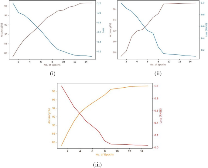
Accuracy and loss curves for the Kylberg dataset using a Basic CNN (acc.: 96.62%, loss: 0.1127), b VGG-16 (acc.: 97.19%, loss: 0.0528), and c Proposed Model (acc.: 99.71%, loss: 0.0301)
-
B.
Results for Brodatz dataset (Fig. 5)
Fig. 5 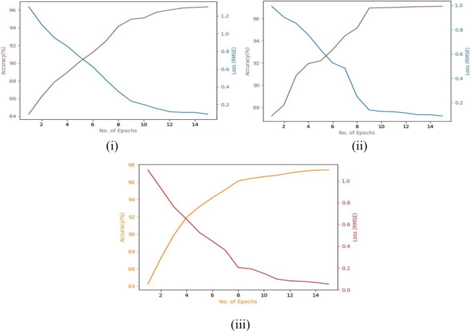
Accuracy and loss curves for the Brodatz dataset using i Basic CNN (acc.: 96.37%, loss: 0.1309), ii VGG-16 (acc.: 97.12%, loss: 0.0767), and iii Proposed model (acc.: 97.43%, loss: 0.0391)
-
C.
Results for outex dataset (Fig. 6)
Fig. 6 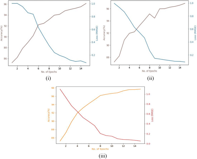
Accuracy and loss curves for the Outex dataset using i Basic CNN (acc.: 96.12%, loss: 0.0945), ii VGG-16 (acc.: 96.89%, loss: 0.0492), and iii Proposed Model (acc.: 97.70%, loss: 0.0396)


In Figs. 4(i, ii), 5(i, ii), 6(i, ii) the purple line indicates the accuracy curve and the blue line indicates the loss curve.
In Fig. 4(iii), 5(iii), and 6(iii) the orange line represents the accuracy curve and the red line represents the loss curve.
The summary of the performance of various models over the three benchmark datasets is represented by Table 6. Table 7 represents the detailed results obtained by applying our model to these three datasets (Figs. 5, 6).
The summary of performance comparison of our technique with the models based on LBP descriptors, Extreme Learning Machine, and other statistical techniques [25,26,27,28,29] is represented by Tables 8, 9 and 10.
It is clear from the results that our method gives better results than most of the other existing models for the Kylberg and Outex TC-12 datasets, and gives competitive results for the Brodatz dataset.
6 Conclusion and future enhancement
In this paper, we have proposed a novel methodology for finding the optimal structure of a deep CNN for the task of texture recognition. Our methodology applies the concept of WOA for optimizing the values of the filters in the convolutional layer, and the values of the weights and biases in the dense layer. For testing the performance of our method, we have applied it to the three different benchmark datasets viz. Kylberg v1.0, Brodatz, and Outex_TC_00012. The results indicate that our model gives better results than most of the existing methods for the Kylberg and Outex_TC_00012 datasets and achieves competitive classification accuracy for the Brodatz dataset. We conclude that our approach helps in making the CNN more robust, and is an effective method for the task of texture recognition.
Our future work includes the utilization of the other recently proposed swarm-intelligence algorithms for optimizing the structure of the CNN. There is immense scope for enhancing this research by applying our model to other pattern recognition tasks like traffic sign recognition, handwritten character recognition, gait recognition, medical image classification, etc.
References
Lu Y, Yi S, Zeng N, Liu Y, Zhang Y (2017) Identification of rice diseases using deep convolutional neural networks. Neurocomputing 267:378–384
Roth HR, Lee CT, Shin HC, Seff A, Kim L, Yao J, Lu L, Summers RM (2015) Anatomy-specific classification of medical images using deep convolutional nets. In: IEEE 12th ISBI, pp 101–104
Basu S, Mukhopadhyay S, Karki M, DiBiano R, Ganguly S, Nemani R, Gayaka S (2018) Deep neural networks for texture classification—a theoretical analysis. Neural Netw 97:173–182
Cimpoi M, Maji S, Vedaldi A (2015) Deep filter banks for texture recognition and segmentation. In: Proceedings of the IEEE conference on computer vision and pattern recognition, pp 3828–3836
Andrearczyk V, Whelan PF (2016) Using filter banks in convolutional neural networks for texture classification. Pattern Recogn Lett 84:63–69
Zhang H, Xue J, Dana K (2017) Deep ten: texture encoding network. In: Proceedings of the IEEE conference on computer vision and pattern recognition, pp 708–717
Mirjalili S, Lewis A (2016) The whale optimization algorithm. Adv Eng Softw, 95:51–67. ISSN 0965-9978. https://doi.org/10.1016/j.advengsoft.2016.01.008
Ma H, Shen S, Yu M, Yang Z, Fei M, Zhou H (2019) Multi-population techniques in nature inspired optimization algorithms: a comprehensive survey. Swarm Evolut Comput 44:365–387
Al-Zoubi AM, Faris H, Alqatawna J, Hassonah MA (2018) Evolving support vector machines using whale optimization algorithm for spam profiles detection on online social networks in different lingual contexts. Knowl Based Syst. Available online 23 April 2018. ISSN 0950-7051. https://doi.org/10.1016/j.knosys.2018.04.025
Mafarja M, Mirjalili S (2018) Whale optimization approaches for wrapper feature selection. Appl Soft Comput, 62:441–453. ISSN 1568-4946. https://doi.org/10.1016/j.asoc.2017.11.006
Sun WZ, Wang JS (2017) Elman Neural network soft-sensor model of conversion velocity in polymerization process optimized by chaos whale optimization algorithm. IEEE Access 5:13062–13076
Aljarah I, Faris H, Mirjalili S (2018) Optimizing connection weights in neural networks using the whale optimization algorithm. Soft Comput 22(1):1–15
Bhardwaj A, Tiwari A, Bhardwaj H, Bhardwaj A (2016) A genetically optimized neural network model for multi-class classification. Expert Syst Appl 60:211–221
Qian S, Liu H, Liu C, Wu S, Wong HS (2018) Adaptive activation functions in convolutional neural networks. Neurocomputing 272:204–212. ISSN 0925-2312. https://doi.org/10.1016/j.neucom.2017.06.070
Trivedi A, Srivastava S, Mishra A, Shukla A, Tiwari R (2018) Hybrid evolutionary approach for Devanagari handwritten numeral recognition using convolutional neural network. Procedia Comput Sci 125:525–532. https://doi.org/10.1016/j.procs.2017.12.068
Pan SJ, Yang Q (2010) A survey on transfer learning. IEEE Trans Knowl Data Eng 22:1345–1359
Lopes UK, Valiati JF (2017) Pre-trained convolutional neural networks as feature extractors for tuberculosis detection. Comput Biol Med. https://doi.org/10.1016/j.compbiomed.2017.08.001
Kylberg G The Kylberg Texture Dataset v. 1.0, Centre for Image Analysis, Swedish University of Agricultural Sciences and Uppsala University, External report (Blue series) No. 35. http://www.cb.uu.se/gustaf/texture/
Brodatz texture image database (2014) [Online]. http://www.ux.uis.no/~tranden/brodatz.html
USC-SIPI Image Database (1977) http://sipi.usc.edu/database/
Brodatz P (1966) Textures: a photographic album for artists and designers. Dover Publications, New York
Outex Database, Center for Machine Vision Research Department of Computer Science and Engineering, University of Oulu, Finland http://www.outex.oulu.fi/index.php?page=test_suites
Ojala T, Mäenpää T, Pietikäinen M, Viertola J, Kyllönen J, Huovinen S (2002) Outex—new framework for empirical evaluation of texture analysis algorithms. In: ICPR, pp 701–706
Simonyan K, Zisserman A (2015) Very deep convolutional networks for large-scale image recognition in ICLR. https://www.robots.ox.ac.uk/~vgg/publications/2015/Simonyan15/simonyan15.pdf
Tensorflow API, Google Brain, Apache License 2.0, Nov. 15. https://www.tensorflow.org/api_docs/
Y Kaya, ÖF Ertuğrul, R Tekin (2015) Two novel local binary pattern descriptors for texture analysis. Appl Soft Comput 34:728–735. ISSN 1568-4946. https://doi.org/10.1016/j.asoc.2015.06.009
El Khadiri I, Kas M, El Merabet Y, Ruichek Y, Touahni R (2018) Repulsive-and-attractive local binary gradient contours: new and efficient feature descriptors for texture classification. Inf Sci. https://doi.org/10.1016/j.ins.2018.02.009
de Mesquita Sá Jr. JJ, Backes AR (2016) ELM based signature for texture classification. Pattern Recognit 51:395–401. ISSN 0031-3203. https://doi.org/10.1016/j.patcog.2015.09.014
Ahmadvand A, Daliri MR (2016) Invariant texture classification using a spatial filter bank in multi-resolution analysis. Image Vis Comput 45:1–10. ISSN 0262-8856. https://doi.org/10.1016/j.imavis.2015.10.002
Pan Z, Li Z, Fan H, Wu X (2017) Feature based local binary pattern for rotation invariant texture classification. Expert Syst Appl 88:238–248. ISSN 0957-4174. https://doi.org/10.1016/j.eswa.2017.07.007
Author information
Authors and Affiliations
Corresponding author
Ethics declarations
Conflict of interest
The authors declare that they have no conflict of interest.
Additional information
Publisher's Note
Springer Nature remains neutral with regard to jurisdictional claims in published maps and institutional affiliations.
Rights and permissions
About this article

Cite this article
Dixit, U., Mishra, A., Shukla, A. et al. Texture classification using convolutional neural network optimized with whale optimization algorithm. SN Appl. Sci. 1, 655 (2019). https://doi.org/10.1007/s42452-019-0678-y
Received:
Accepted:
Published:
DOI: https://doi.org/10.1007/s42452-019-0678-y