
Abstract
Cross-projects software defect prediction improves the quality of new software projects or projects with a shortage of historical data. Therefore, various data mining techniques are recommended in this field. The classification accuracy issue is considered one of the most significant problems due to the shortage and heterogeneous in historical data. To address this challenge, this research utilizes a spotted hyena optimizer algorithm as a classifier to predict defects through cross-projects. Confidence and Support are utilized as a multi-objective fitness function to look for the best classification rules. These classification rules are used to predict defects for new projects or other projects with insufficient data. The datasets of NASA such as JM1, KC1, and KC2 are used. By applying spotted hyena optimizer algorithm as a classifier on one dataset and predicting defects in the other two datasets, accuracy is reported 84.6, 92.0, 82.4, 90.7, 86.6 and 81.8 for JM1, KC1, and KC2 respectively. These accuracy values are better than the most significant data mining techniques in the field such as Support Vector Machine, Naïve Bayes, Boosting, C4.5, and Bagging. Also, the proposed research discusses other performance measures such as precision, recall, and f-measure. The conclusion proves that there are many features of McCabe and Halstead that have a strong impact to generate highly accurate predictors for defects such as McCabe’s line count of code, McCabe’s cyclomatic complexity, McCabe’s essential complexity, McCabe’s design complexity iv, Halstead’s effort, Halstead’s time estimator, Halstead’s line count, Halstead’s count of line of comments and total operators.
1 Introduction
Nowadays, Software Defect Prediction (SDP) is very critical in software engineering and one of the most helping activities during the testing phase of the System Development Life Cycle (SDLC). However, predicting the defective modules isn’t a straight forward job [1].
Defects of software are errors, flaws, mistakes, faults or bugs in software. They may come from the absence of developer experience, the misconception of requirements or uncontrollable development phase which will produce failures or unexpected results [2].
The quality and reliability of the software are demanded to meet user requirements in constrained timespan by identifying and predicting defects in the early stage of SDLC. Therefore, SDP models help teams of quality assurance to allocate resources to the most defective modules [2,3,4].
Generally, there are three approaches in SDP models.
-
With-in project SDP: SDP model is built by gathering historical data from a project of software (training phase) and predicts defects in the same project (testing phase) i.e. training and testing phases are applied on the same project. However, projects that have no historical data cannot be applied. Therefore, accuracy cannot be achieved [5].
-
Cross-projects SDP for similar datasets: SDP model is utilized in a mode such that historical data of projects isn’t presented or insufficient to train and build the SDP model. The SDP model is trained and developed on one project and applied for cross projects or other projects. The drawback here is that it requires projects with the same features and metrics [5].
-
Cross-projects SDP for heterogeneous or dissimilar datasets: SDP model is presented to predict defects with disparate datasets [5].
Recent researches use data mining methodologies that depend on machine learning as important models. Many techniques were used in SDP such as Support Vector Machine (SVM) [6], Naïve Bayes (NB) [7], Boosting [8], C4.5 [9] and Bagging [10]. SDP models still suffer from a very important and challenging issue, which is detecting accuracy [11, 12].
This research uses an algorithm called Spotted Hyena Optimizer (SHO) [13] as a classifier model for predicting software defects in cross projects for similar metrics in different datasets. SHO is developed and trained on one project and applied for predicting software defects in other projects (cross projects) with the same features and metrics. To locate the most fitness classification rules, the experiments apply confidence (CONF) and support (SUP) as a multi-objective function on one project with historical data to build the SDP model and apply these classification rules on other projects that don’t have a sufficient historical data such as new projects. Moreover, it assists software engineering industries to upgrade quality in limited time and effort during the development process.
In this research, SHO is used for the first time as a classifier with a multi-objective fitness function of CONF and SUP. This algorithm makes accuracy values better than the most significant data mining techniques in the field. SHO is utilized as a feasible meta-heuristic algorithm in terms of complexity and efficiency as compared to other traditional algorithms. It has been utilized for obtaining the acceptable solutions for different design problems [13]. In the previous researches, there is a shortage study on the accuracy of traditional cross-project SDP models for similar datasets. Therefore, the experiment study uses SHO as a classifier using (CONF) and (SUP) as a multi-objective fitness function on one project with historical data to build the SDP model. The previous step results the most fitness classification rules used in other projects that don’t have a sufficient historical data such as new projects.
The rest of this research is composed as follows: Sect. 2 describes recent techniques for predicting software defects. Section 3 discusses the SHO algorithm and its mathematical model. Section 4 presents a brief discussion of the proposed classifier. Section 5 shows the discussion and experimental study of the proposed algorithm. Finally, Sect. 6 lists the conclusion and future work.
2 Literature survey
Manual testing requires 27% of development effort [14] furthermore; it couldn’t detect all defects of software. Also, With-in project SDP still suffers from classification accuracy because there are new projects without historical data used to build the SDP model. Hence, cross-projects SDP is considered one of the most significant activities in producing defect-free products of software. It reduces the time and effort of testing teams. This section discusses the common related work of cross-projects SDP with a similar dataset.
It is commonly favored for SDP to learn utilizing the locally accessible data of a software project (within–projects SDP). This local data is obtained from the historical versions and forms of the project. With-in projects SDP model is constructed by gathering historical data from a software (training phase) and predicts defects in the same software (testing phase). This approach suffers from different challenges such as how to predict defects in new projects with a shortage in historical data? Therefore, accuracy cannot be achieved. Nevertheless, the challenge of unavailability of the local data faces the organization’s team. The reasons for unavailability may be due to the changing of technology or no similar features of projects previously developed [1]. To overcome this problem, the cross-project software defect prediction is used. It is utilized in a mode such that historical data of projects isn’t presented or insufficient to train and build a SDP model. Therefore, the SDP model is trained and developed on one project and is applied for cross projects or other projects provided the projects have the same features and metrics [5]. The cross-projects SDP is a classification model that is composed of a set of rules for prediction gathered on the training phase.
Steffn Herbold [15] presented research that provided a benchmark of 26 cross-projects software defect prediction methodologies depended on cost metrics. His benchmark demonstrated that expecting everything as defective was on average better than cross-projects software defect prediction under cost considerations. Moreover, the research demonstrated that the rank of methodologies utilizing metrics of cost was uncorrelated to the rank depended on the metrics that don’t utilize costs.
Fei Wu et al. [16] presented a solution that was effective and unified for both semi-supervised cross-project software defect prediction and semi-supervised with-in software defect prediction problems. This research presented a learning technique of semi-supervised technique and proposed a cost-sensitive kernelized semi-supervised dictionary learning technique.
Yun Zhang et al. [17] researched seven composite techniques that coordinate several classifiers of machine learning to enhance cross-projects software defect prediction. For evaluating the composite algorithms, they applied the experiments on 10 software systems (open source) from the PROMISE repository [18]. The research compared the composite techniques with a combined SDP model where meta- classification used logistic regression using F-measure and cost metrics for evaluation. The experiment shows that the proposed algorithms are better in performance than the compared algorithm.
Peng He et al. [19] developed TD selector using defects and similarity as a weighted function. He utilized logistic regression as a classifier model and analyzed the effects of several combinations of normalization and similarity of defects on the performance of prediction. Also, he compared it with the other two methods. The experiments are applied to 14 projects gathered from public repositories.
Chao Ni et al. [20] proposed a cluster-based strategy feature extraction utilizing clusters of hybrid-data to ease the conveyance contrasts. It incorporates two stages. The strategy of clustering basing on density is used by the feature clustering stage to cluster features. Also, the strategy of ranking is used by feature extraction. For cross-project software defect prediction, the research designed three several heuristic ranking methods in the second stage. The experiment is applied to real-world projects.
Thomas Zimmermann et al. [21] studied cross-projects software defect prediction models on an extensive scale. For 22 real applications, they ran 622 cross-projects software defect prediction. The results demonstrated that cross-projects software defect prediction didn’t lead to perfect or accurate predictions.
As indicated by the previous work, there is an expanding requirement for predicting the software defects with a shortage of historical data. Besides, this detection is required at the starting time of the software development life cycle due to the high maintenance cost. Therefore, the proposed research aims at enhancing cross-projects software defect prediction that still suffers from different challenges and drawbacks such as detecting accuracy [12] and solving the problem of how to predict defects in new projects with a shortage in historical data? Moreover, the proposed cross-project software defect prediction model utilizes the SHO algorithm [13] as a classifier. SHO algorithm was not used as a classifier before especially in this field. In addition to, CONF and SUP were not used as multi-objective fitness functions with the SHO algorithm for classification. Therefore, the performance of the algorithm and accuracy are increased. The convergence of the SHO in this research converges around 4% of the all-out number of cycles. Therefore, the best fit rule is met at less time. The following section explains the spotted hyena optimizer algorithm.
3 Spotted hyena optimizer (SHO)
Algorithms of meta-heuristic are summarized into three categories physical, evolutionary and swarm-based [22]. SHO [13] is a meta-heuristic algorithm motivated by the behavior of the spotted hyena. SHO is scored with one unconstrained and 5 constrained problems of engineering design: loaded structure displacement, speed reducer, welded beam, pressure level, compression spring, and element of rolling bearing [13, 36]. SHO is also used in classification of heart problem [37]. The principle thought of the SHO is the social association among hyenas and their conduct. SHO mathematically modeled the three stages of spotted hyena’s behavior: looking for, surrounding and assaulting prey. The SHO is better in performance over the other meta-heuristic algorithms. The following subsections summarize the mathematical model of encircling, hunting and exploiting the prey by the spotted hyenas.
3.1 Encircling the prey
Dhiman et al. [13] mathematically demonstrated the spotted hyenas’ hierarchy. They consider the prese nt best solution is the objective target which is near the ideal because of search space not known a priori. The other search hyenas will attempt to refresh their situations after the best search solution is characterized. The following equations explain the model of encircling prey:
where \({\vec{\text{D}}}_{\text{h}}\) describes the partition among the spotted hyena and prey, x represents the present iteration, \({\vec{\text{B}}}\) and \({\vec{\text{E}}}\) are vectors of co-efficient, \({\vec{\text{P}}}_{\text{p}}\) represents the prey position vector and \({\vec{\text{P}}}\) is the position vector of spotted hyena. || shows the absolute value and × is the multiplication with vector. The vectors \({\vec{\text{B}}}\) and \({\vec{\text{E}}}\) are computed as follow:
where iteration = 1, 2, 3…, \({\text{Max}}_{\text{iteration}}\). For legitimate changing the mode of exploitation and exploration, \(\overrightarrow {\text{h }}\) directly diminishes from 5: 0 through \({\text{Max}}_{\text{iteration}} ,r\vec{d}_{1} ,r\vec{d}_{2}\), are irregular vectors in [0, 1].
3.2 Hunting the prey
Spotted hyenas commonly live and pursue in gatherings and depend upon an arrangement of partners and the ability to see the region of prey. For describing the behavior of spotted hyena mathematically, they consider the most feasible search agent, which ideally knows the area of prey. The other individuals make a gathering towards the perfect individual.
The following equations present the mathematical model of hunting prey:
where \(\vec{P}_{h}\) is describes as the situation of first feasible hyena, \(\vec{P}_{k}\) demonstrates the situation of other agents. Here, N represents the number of hyenas which is expressed as follow:
where \({\vec{\text{M}}}\) is an irregular vector in [0.5, 1], nos represents the number of solutions and \({\vec{\text{C}}}_{\text{h}}\) is a cluster of N number of ideal solutions.
3.3 Exploiting the prey
To show the model for attacking the prey, they decrease the vector \(\overrightarrow {\text{h }}\) value; the variety in the vector \({\vec{\text{E}}}\) is also decreased to change the value in the vector \(\overrightarrow {\text{h }}\) which could decline from 5 to zero through the iterations. The following equation represents the model of attacking prey:
where \({\vec{\text{P}}}\left( {{\text{x}} + 1} \right)\) saves the most feasible and updates the locations of other agents. The next section explains the SHO algorithm as a classifier and how it is utilized to optimize the most accurate classification rules in cross-project SDP for similar datasets.
4 Proposing SHO as a classifier
In new projects, Cross-projects software defect prediction is viewed as a standout amongst the essential tasks in software engineering due to the shortage in historical data [23][24]. Also, accuracy can’t be fulfilled and problems of real-life may increase such as efficiency and complexity. Detecting accuracy still can’t be achieved through with-in SDP; especially new projects. Sections 1 and 2 briefly discuss how with-in SDP and cross-projects SDP would depend on machine learning. Hence, there is an increasing need to obtain optimal solutions by meta-heuristic techniques [22].To face this challenge, this research utilizes the SHO algorithm as a classifier for predicting defects in a mode such that historical data of projects isn’t presented or insufficient to train and build a SDP model.
The following figure demonstrates the flow of data and essential processes in the SHO classifier through cross-projects SDP as following:
-
The instances are built from software archives such as version control. Each instance represents class, file, package or method which is defective or not.
-
This research uses the discretization process for dataset via RapidMiner 5.3 tool [25] because the exact matching among instances of datasets and individuals of the population is very difficult. Hence, the SUP and CONF degrees help the multi-objective function to assess the perfect rules of classification.
-
The SHO that used as a classifier repeats the search for the fit rule (classification rules) depending on a random subset of a dataset of a project (dataset of training).
-
For new projects with similar datasets that can’t present historical data, the classification rules resulted from the training phase are used to predict the defects (Fig. 1).
Fig. 1 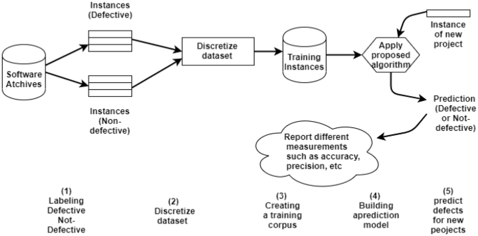
Cross-projects SDP model utilizing SHO as a classifier
-
According to results, a report of accuracy, F-measure, specificity, recall, and precision are calculated for comparing with other techniques of data mining such as Artificial Neural Network (ANN), Support Vector Machine, Naïve Bayes, Bagging, Random Forest, K nearest neighbors (K-NN), and C4.5.

The following subsections explain the multi-objective fitness function, phases, and flow chart.
4.1 Multi-objective fitness function
Objective function [26] evaluates how to find the most fitness solution of the presented issue. During the experiments, this subsection that explains the confidence and support [27] as a multi-objective function is utilized to find the perfect rules of classification. First, SUP of the rule is calculated by how many instances that fulfill the rule. It can be expressed as follow:
Second, CONF is calculated. It is the proportion of the number of instances occurrence that satisfies the entire rule (antecedents and consequences) to the number of instances occurrence that satisfies only the antecedent. It can be described as follow:
where \(COUNT\_SS\) is the number of instances that satisfies the rule, R is the total number of instances in the dataset and \(COUNT\_CC\) is the number of instances that fulfill the antecedent of the rule.
Finally, the multi-objective fitness function (FT) for each rule is calculated as follow:
where \(W_{1} \;{\text{and}}\;W_{2}\) are weights given to the SUP and CONF functions depending on their relative significance.
4.2 Flowchart and phases of the SHO as a classifier
In this subsection, the phases of the SHO as a classifier through cross-projects SDP and the multi-objective fitness function.
As indicated in Fig. 2:

Flow chart of the SHO classifier through cross-projects SDP
-
Create a population of spotted hyenas and pick the initial parameters.
-
Apply the combination of SUP and CONF that used as a multi-objective function for each individual of the spotted hyenas to assess the desired classification rules.
-
Then, the position of each hyena is refreshed by attempting to learn from the spotted hyena with maximum multi-objective fitness function (SUP and CONF).
-
After that, the SHO repeats to search for best-spotted hyena (classification rules) depending on a random subset of a dataset of a project (training phase). The resulted classification rules are utilized as input for prediction and classification processes on other new projects with a shortage of historical data.
This research bases on the steps indicated in algorithm 1 to explain the stages of the SHO as a classifier through cross-projects SDP. Moreover, this research answers the question of how to predict instances (defective or not) of new projects and projects that have a shortage in historical data (cross-projects SDP) using SUP and CONF concepts as a multi-objective fitness function.
First, the SHO classifier calculates the initial parameters as indicated in algorithm 1 where parameters are adjusted and initialized (pop = population size = 500, F = number of features or metrics = 22 and MaxIter = maximum number of iterations = 50). Then for each agent of spotted hyena, the multi-objective fitness function is calculated. During the optimization process, SUP and CONF of classification rules are utilized as indicated in Eqs. 11, 12, 13. It helps SHO to be used as a classifier by looking for the suitable classification rules between initially spotted hyenas (random rules). SHO repeats to find the best classification rules. After that, the best solutions are clustered. Then, the position of the spotted hyena is updated via checking if any agent goes past the farthest point and change it. The values of new parameters and the multi-objective fitness function of the updated agent are calculated again. Finally, the SHO returns the best classification rules that are used for predicting defects in new projects or projects with a shortage of historical data. Therefore, this is called cross-projects SDP.

5 Experimental study
This section discusses the study of SHO as a classifier through a cross-projects approach in the SDP field utilizing SUP and CONF as a multi-objective fitness function.
5.1 Experiment setup
This research experiments utilized the following tools and features:
-
RapidMiner 5 tool [25] is used for the discretization process.
-
The simulation tool of MATLAB [28] is utilized during the implementation process.
-
PROMISE [18] and OPENML[29] websites of open-source datasets.
-
WEKA 3.6 tool [30] for comparisons.
-
PC with CPU Intel(R) Core (TM) i5 and RAM (4 GB).
KC1, JM1, and KC2 are datasets of NASA metrics related to defects of data program. They are for receiving and processing management of data storage [29]. They are included various features that are utilized through experiments from the archive of OPENML [29] and PROMISE [18]. Table 1 indicates various dataset parameters where software components, software features, number of defects and percentage of defects. Common metrics of datasets are indicated in Table 2. These metrics are useful since it can generate a predictor with high accuracy for defects, easy to use as they can be gathered and collected cheaply and automatically such as lines of code (LOC) and widely used as many researchers utilize static features for guiding quality of software prediction [18, 29, 33, 34]. By utilizing these datasets, SHO that used as a classifier is trained to extract suitable classification rules for predicting defects through new projects or projects that don’t have sufficient historical data (cross-projects SDP). Accuracy of classification and precision are the most popular measurements compared with other techniques in WEKA 3.6 tool data mining.
The matrix that the experiment depends on is called a confusion matrix [31]. As is shown in Table 3, it is a table that is routinely used to describe the performance of the classification model. It has the value of predicted and actual class labels. In Table 3, there are 4 possible outcomes of SHO classifier:
-
True Positives (TP):- defective modules are classified correctly as defective.
-
False Positives (FP):- non-defective modules are classified incorrectly as defective.
-
True Negatives (TN):- non-defective modules are classified correctly as non-defective.
-
False Negatives (FN):- defective modules are classified incorrectly as non-defective.
Different measurements that belong to data mining techniques such as F-measure, sensitivity (S), recall, precision (P), specificity (SP), and accuracy (ACC) [2] are calculated using the confusion matrix.
Another measurement is specificity (SP) which is expressed as follow:
The next measurement is sensitivity (S). It can be expressed as follow:
Then the precision (P) is calculated and expressed as follow:
F-measure (F_M) is calculated as follow:
Finally, calculating the weighted average (W_A) of each measurement is expressed similar to the following equation:
where \(F\_M_{c1}\) and \(F\_M_{c2}\) are F-measure for class1 and 2 respectively. Also \(N_{c1}\) and \(N_{c2}\) are a number of instances in class1 and 2. \(N_{c1 + c2}\) is the total number of instances in the dataset.
Convergence rate [32] is also another common measure of the optimization algorithm (SHO). Convergence characterizes solutions sequence got through the cycles until it meets a suitable point at less time.
5.2 Experimental results
This section depicts the precision and accuracy classification of the SHO through cross-projects SDP.
-
SHO algorithm is applied and trained as a classifier on one dataset to extract the best classification rules.
-
SHO algorithm is executed 15 runs using a percentage split technique on a trained dataset (60%) and random instances of the other datasets for testing.
-
Predict cross-projects SDP (other datasets mentioned above) by using classification rules extracted from the previous step.
-
The convergence of the SHO in finding the classification model characterizes the relationship between the iterations and values of the multi-objective fitness function.
5.2.1 Training case 1: KC1
“KC1” contains 2109 instances, 22 attributes and 326 defects where 15.5% is defective. The SHO algorithm as a classifier is applied for training to extract the best classification rules by using SUP and CONF as multi-objective fitness functions. Then, classification rules are utilized to predict software defects of random instances in other projects (JM1, KC2) datasets (cross-projects). Here, the confusion matrix is extracted for predicting random instances of JM1 and KC2 datasets as shown in Tables 4 and 5 respectively. These tables discuss the performance of the SHO algorithm as a classifier which trained on the KC1 dataset and test by random instances of other datasets (JM1, KC2). Then, the weighted average for each performance measure is calculated such as precision and accuracy.
These measurements of SHO as a classifier are compared with other data mining techniques as indicated in Tables 6 and 7 such as SVM, NB, ANN, C4.5, principle component analysis algorithm (PCA) for reducing features followed by ANN, K-NN and random forest via WEKA 3.6 tool.
According to Tables 6 and 7, values of SHO classifier such as the weighted average of accuracy, specificity, precision, recall, false-positive rate, and f-measure are resulted from Tables 4 and 5 using equations from 14 to 19. Also, these values that belong to Tables 6 and 7 are resulted by training the SHO algorithm as a classifier and applying the resulted best classification rules on random instances of JM1 and KC2 datasets respectively.
Figure 3 and 4 show the comparison results for precision and accuracy. They indicate the SHO algorithm as classifier used through training in KC1 and applying the resulted classification rules on JM1 and KC2 datasets respectively. The results report the values of precision using the SHO as a classifier (82.2 and 91.6) and values of accuracy (82.4 and 90.7) for JM1 and KC2 respectively. Therefore, the SHO algorithm as a classifier is the best in terms of precision and accuracy through cross-projects SDP. The SHO algorithm converges and meets a suitable point (best rule) after 30% of cycles.

Comparison between SHO classifier and other techniques (train KC1, predict JM1)

Comparison between SHO classifier and other techniques (train KC1, predict KC2)
5.2.2 Training case 2: JM1
“JM 1” contains10885 instances, 22 attributes, and 2106 defects where 19.34% is defective. Tables 8 and 9 indicate the confusion matrix resulted from training the SHO algorithm as a classifier on the JM1 dataset and applying the resulted classification rules on KC1 and KC2 respectively.
Also, the confusion matrix for KC1 and KC2 datasets are given in Tables 8 and 9 which lead to Tables 10 and 11 respectively. These tables and Fig. 5 and 6 indicate the results of the performance measure explained above. These report the values of precision using the SHO as classifier (87.0 and 92.7) and values of accuracy (84.6 and 92.0) for KC1 and KC2 respectively when trained on JM1. Therefore, the SHO algorithm as a classifier is the best in terms of precision and accuracy through cross-projects SDP. The SHO converges after around 8% of the cycles that is a considerably high rate to meet the best fit rules.

Comparison between SHO classifier and other techniques (train JM1, predict KC1)

Comparison between SHO classifier and other techniques (train JM1, predict KC2)
5.2.3 Training case 3: KC2
“KC2” contains 522 instances, 22 attributes, and 107 defects where 20.5% is defective. Tables 12 and 13 indicate the confusion matrix resulted from training the SHO algorithm as a classifier on the KC2 dataset and applying the resulted classification rules on KC1 and KM1 respectively.
Similarly, Tables 14, 15 and Figs. 7, 8 indicate the results of performance measures. These report the values of precision using the SHO as a classifier (84.8 and 85.1) and values of accuracy (86.6 and 81.8) for KC1 and JM1 respectively when trained on KC2. Therefore, the SHO algorithm as a classifier is the best in terms of precision and accuracy through cross-projects SDP. The convergence of the SHO achieved around 8% of the cycles. Therefore, the best fit rule is met at less time.

Comparison between SHO classifier and other techniques (train KC2, predict KC1)

Comparison between SHO classifier and other techniques (train KC2, predict JM1)
The next table presents the descriptive statistics of the SHO as a classifier in terms of accuracy. SHO algorithm is executed around 15 times using a percentage split technique on a trained dataset (60%) and random instances of the other datasets for testing (Table 16).
Table 17 represents the standard deviation for each algorithm. The lowest error is the SHO algorithm as a classifier most of the time. If there is a tie in two algorithms in terms of accuracy, the error rate will help to break the tie. The lower the error is the higher the accuracy.
5.3 Experimental discussion
According to the previous section, the features of datasets utilized in this research are extracted from:-
-
McCabe feature extractor of source code which argues that code with complicated pathways is more error-prone. Therefore his metrics reflect the pathways within a code module [33].
-
Halstead feature extractor of source code which argues that code that is hard to read is more likely to be fault-prone. It estimates reading complexity by counting the number of concepts in a module e.g. number of unique operators [34].
These features describe code features that are related to the quality of the software. The McCabe and Halstead measures are module based (Function or Method) where is the smallest unit of functionality [35]. These features are studied since they are useful, easy to use, and widely used.
The experiments (Case 1, 2 and 3) prove, there are many features of McCabe and Halstead that have a strong impact to generate highly accurate predictors for defects such as McCabe’s line count of code (LOC), McCabe’s cyclomatic complexity v(g), McCabe’s essential complexity ev(g), McCabe’s design complexity iv(g), Halstead’s effort (e), Halstead’s time estimator (t), Halstead’s line count (LOCode), Halstead’s count of line of comments (LOComment) and total operators (Total_op). The other features don’t have the same impact degree in generating highly accurate predictors for defects such as Halstead’s volume (v), total operands (total_opnd), unique operators (unique_op) and unique operands (unique_opnd).
The experiments (Case 1, 2 and 3) prove that the SHO classifier through cross-projects SDP is better than other techniques in terms of precision and accuracy with an average 87.3 and 86.4 respectively.
General limitations of meta-heuristic search algorithms are the convergence speed and long computational time. SHO proved its ability to overcome these limitations. Figure 9 is the convergence of the SHO algorithm in finding the SDP classification model. The figure characterizes the relationship between the algorithm iterations and values of the multi-objective fitness function during one run from the experiments. The SHO algorithm converges after 4 iterations out of 50 iterations which is a very fast convergence rate i.e. it meets a suitable point (best rule) at less time. SHO algorithm is executed 15 runs using a percentage split technique on a trained dataset (60%) and random instances of the other datasets for testing.

The convergence rate of SHO
6 Conclusion and future work
Recently, SDP is introduced as an emergent issue in software engineering industries. Various techniques are presented for enhancing SDP. The enhancement faced the issue of shortage in historical data. This research proposed a feasible solution for cross-projects SDP using the SHO algorithm as a classifier. The classification accuracy is determined by training the SHO algorithm as a classifier on one dataset of projects and applying the resulted classification rules on different projects. SUP and CONF are utilized as a multi-objective fitness function to identify suitable classification rules. Experimental results indicate that the SHO classifier is better than other techniques with an average accuracy of 86.4%. Moreover, precision, specificity, sensitivity, F-measure, and recall are calculated for the SHO algorithm classifier and compared with the other techniques in WEKA 3.6. These experiments demonstrate that the SHO classifier has an efficient ability to predict software defects through cross-projects.
In the future, algorithms for reducing features would be utilized before applying the SHO classifier. The feature reduction algorithms will extract and select the most significant features leading to enhance the classification process. Moreover, using the classifier on cross-projects SDP for heterogeneous or dissimilar Dataset is a fascinating point. Although SHO overcomes some of the meta-heuristic algorithms limitation, more investigation is required for other issues like trapping into local optima, tuning many parameters, difficult encoding scheme and having good performance only in real or binary search spaces.
Change history
31 January 2022
A Correction to this paper has been published: https://doi.org/10.1007/s42452-022-04942-z
References
Arora I, Tetarwal V, Saha A (2015) Open issues in software defect prediction. Proc Comput Sci 46:906–912
Nam J (2014) Survey on software defect prediction. Department of Compter Science and Engineerning, The Hong Kong University of Science and Technology, Tech Rep
Li Z, Jing X-Y, Zhu X (2018) Progress on approaches to software defect prediction. IET Softw 12:161–175
Wei H, Hu C, Chen S, Xue Y, Zhang Q (2019) Establishing a software defect prediction model via effective dimension reduction. Inf Sci 477:399–409
Kalaivani N, Beena R (2018) Overview of Software Defect Prediction using Machine Learning Algorithms. Int J Pure Appl Math 118:3863–3873
Shan C, Chen B, Hu C, et al (2014) Software defect prediction model based on LLE and SVM, Communications Security Conference (CSC 2014)
Okutan A, Yıldız OT (2014) Software defect prediction using Bayesian networks. Empir Softw Eng 19:154–181
Aljamaan HI, Elish MO (2009) An empirical study of bagging and boosting ensembles for identifying faulty classes in object-oriented software. In: 2009 IEEE symposium on computational intelligence and data mining. IEEE, pp 187–194
Koru AG, Liu H (2005) Building effective defect-prediction models in practice. IEEE Softw 22:23–29
Kuncheva LI, Skurichina M, Duin RPW (2002) An experimental study on diversity for bagging and boosting with linear classifiers. Inf Fusion 3:245–258
Jayanthi R, Florence L (2019) Software defect prediction techniques using metrics based on neural network classifier. Cluster Comput 22:77–88
Kaur R, Sharma ES (2018) Various techniques to detect and predict faults in software system: survey. Int J Futur Revolut Comput Sci Commun Eng (IJFRSCE) 4:330–336
Dhiman G, Kumar V (2017) Spotted hyena optimizer: a novel bio-inspired based metaheuristic technique for engineering applications. Adv Eng Softw 114:48–70
Raukas H. Some approaches for software defect prediction, Bachelor’s Thesis (9ECTS), Institute of Computer Science Computer Science Curriculum, University of TARTU
Herbold S (2018) Benchmarking cross-project defect prediction approaches with costs metrics. arXiv Prepr arXiv180104107
Wu F, Jing X-Y, Sun Y et al (2018) Cross-project and within-project semisupervised software defect prediction: a unified approach. IEEE Trans Reliab 67:581–597
Zhang Y, Lo D, Xia X, Sun J (2018) Combined classifier for cross-project defect prediction: an extended empirical study. Front Comput Sci 12:280–296
Tera-PROMISE Home. http://promise.site.uottawa.ca/SERepository/dataetspage.html. Accessed 26 Feb 2018
He P, He Y, Yu L, Li B (2018) An improved method for cross-project defect prediction by simplifying training data. Math Probl Eng. https://doi.org/10.1155/2018/2650415
Ni C, Liu W-S, Chen X et al (2017) A cluster based feature selection method for cross-project software defect prediction. J Comput Sci Technol 32:1090–1107
Zimmermann T, Nagappan N, Gall H, et al (2009) Cross-project defect prediction: a large scale experiment on data vs. domain vs. process. In: Proceedings of the 7th joint meeting of the European software engineering conference and the ACM SIGSOFT symposium on the foundations of software engineering. ACM, pp 91–100
Ren J, Qin K, Ma Y, Luo G (2014) On software defect prediction using machine learning. J Appl Math. https://doi.org/10.1155/2014/785435
Qing H, Biwen L, Beijun S, Xia Y (2015) Cross-project software defect prediction using feature-based transfer learning. In: Proceedings of the 7th Asia-Pacific symposium on internetware. ACM, pp 74–82
Bal PR, Kumar S (2018) Cross project software defect prediction using extreme learning machine: an ensemble based study. In: ICSOFT, pp 354–361
Download Rapidminer Studio|RapidMiner. https://rapidminer.com/get-started/. Accessed 9 Nov 2019
Deb K (2014) Multi-objective optimization. In: Search methodologies. Springer, pp 403–449
Qodmanan HR, Nasiri M, Minaei-Bidgoli B (2011) Multi objective association rule mining with genetic algorithm without specifying minimum support and minimum confidence. Expert Syst Appl 38:288–298
Download MATLAB, Simulink, Stateflow, and Other MathWorks Products. https://www.mathworks.com/downloads/web_downloads/?s_tid=sp_ban_dl. Accessed 9 Nov 2019
OpenML. https://www.openml.org/search?type=data. Accessed 9 Nov 2019
Witten IH, Frank E, Hall MA, Pal CJ (2016) Data Mining: Practical machine learning tools and techniques. Morgan Kaufmann
Sammut C, Webb GI (2011) Encyclopedia of machine learning. Springer, New York
Cartis C, Scheinberg K (2018) Global convergence rate analysis of unconstrained optimization methods based on probabilistic models. Math Program 169:337–375
McCabe TJ (1976) A complexity measure. IEEE Trans Softw Eng SE-2(4):308–320
Halstead MH (1977) Elements of software science. Elsevier, New York
Runeson P (2006) A survey of unit testing practices. IEEE Softw 23:22–29
Dhiman G, Kumar V (2019) Spotted hyena optimizer for solving complex and non-linear constrained engineering problems BT. In: Yadav N, Yadav A, Bansal JC et al (eds) Harmony search and nature inspired optimization algorithms. Springer, Singapore, pp 857–867
Li J, Luo Q, Liao L, Zhou Y (2018) Using spotted hyena optimizer for training feedforward neural networks. In: International conference on intelligent computing. Springer, pp 828–833
Funding
There is no funding provided and this research is submitted for Partial Fulfillment of the Requirements for the M.Sc. Degree in software engineering at Faculty of Computers and Artificial Intelligence, Helwan University, Egypt.
Author information
Authors and Affiliations
Corresponding author
Ethics declarations
Conflict of interest
The authors declare that they have no conflict of interest. They work at different Government Universities. Their aim purpose is only Scientific and academic research.
Additional information
Publisher's Note
Springer Nature remains neutral with regard to jurisdictional claims in published maps and institutional affiliations.
The original online version of this article was revised.
In this article, affiliation no. 1 incorrectly showed as the last author's first affiliation
Rights and permissions
About this article

Cite this article
Elsabagh, M.A., Farhan, M.S. & Gafar, M.G. Cross-projects software defect prediction using spotted hyena optimizer algorithm. SN Appl. Sci. 2, 538 (2020). https://doi.org/10.1007/s42452-020-2320-4
Received:
Accepted:
Published:
DOI: https://doi.org/10.1007/s42452-020-2320-4