


A central question in comparative politics—and one of the foundational questions of economics (Smith Reference Smith1776)—asks why some nations have grown, prospered, and developed more rapidly than others. While explanations of differing rates of development range from genetic to biological to geographic to environmental (see Baker Reference Baker2013 or Diamond Reference Diamond1997 for syntheses), major cross-national research projects argue persuasively that political competition lies at the heart of this story (Acemoglu et al. Reference Acemoglu, Naidu, Restrepo and Robinson2019; Acemoglu and Robinson Reference Acemoglu and Robinson2006; Ansell Reference Ansell2010; Bollyky et al. Reference Bollyky, Templin, Cohen, Schoder, Dieleman and Wigley2019; Lindert Reference Lindert2004; North, Wallis, and Weingast Reference North, Wallis and Weingast2009; Paglayan Reference Paglayan2021; Stasavage Reference Stasavage2005). Comparative politics has shown that varied political institutions can set nations on different trajectories in the educational levels, wealth, and well-being of their residents.
Yet in the field of American state politics—an arena where, unlike in the international realm, we can examine variation among states that are all, at least nominally, democratic—this question has been all but ignored. This is not because the American states lack variation in levels of prosperity or health or education. But why have some states prospered, while others have faltered? What set some states on a path to higher growth, a broader expansion of educational opportunities, or an earlier elimination of illiteracy? Why have some states been able to reduce infant mortality rates more sharply than others and even seen something as essential as the life expectancies of their residents grow more rapidly?
Few scholars have taken up these questions. Those who have are primarily economists, and they have focused almost exclusively on growth in income levels (Besley and Case Reference Besley and Case2003; Besley, Persson, and Sturm Reference Besley, Persson and Sturm2010; Frank Reference Frank2009; Goldberg, Wibbels, and Mvukiyehe Reference Hixson, Hepler and Kim2008; Malloy, Pearson-Merkowitz, and Morris Reference Malloy, Pearson-Merkowitz and Morris2016; Mitchener and McLean Reference Smith2003) rather than the broader notion of human development described in the work of Amartya Sen (Reference Sen1999). Political scientists have done landmark research detailing the differences in policy choices across states (Brown Reference Brown1995; Caughey and Warshaw Reference Caughey and Warshaw2017; Caughey, Warshaw, and Xu Reference Caughey, Warshaw and Xu2017; Dawson and Robinson Reference Dawson and Robinson1963; Dye Reference Acemoglu, Naidu, Restrepo and Robinson1966; Hofferbert Reference Hofferbert1966; Rose Reference Rose2013; Schneider Reference Dye1988; Smith Reference Schneider1997; Winters Reference Mitchener and McLean1976), but we have found no work at the state level looking comprehensively at the policy outcomes that these choices bring. While Aldrich and Griffin (Reference Aldrich and Griffin2018) do begin to examine these questions, their units of analysis are regions (North, South, and Border States) rather than individual states.
Our argument is that political institutions in general—and party competition in particular—are central to explaining variations in development across the states. Parties give their members individual electoral incentives to pursue the collective goal of improving the public welfare, at the same time that they create the political ties necessary to move a major policy program through government (Aldrich and Griffin Reference Aldrich and Griffin2018; Key Reference Key1949). When parties compete most fiercely, these incentives and advantages are magnified. Close competition between two parties in a statehouse leads to investments in human capital and infrastructure, with these investments later paying off for the wealth, health, and educational attainment of state residents.
In this new quantitative historical analysis of data on all 50 states, we test whether party competition has—by facilitating public investments—led to more robust levels of economic growth, higher levels of education and literacy, lower infant mortality rates, and longer life spans. We separate our empirical tests into two linked questions. First, does party competition lead states to invest in human capital and infrastructure, spending more on policies promoting education, health, and transportation? Next, following the patterns identified in cities and regions by Cutler and Miller (Reference Cutler and Miller2005), Kunitz (Reference Kunitz2015), and Chetty et al. (Reference Chetty, Stepner, Abraham, Lin, Scuderi, Turner, Bergeron and Cutler2016), do these investments by states pay off in future levels of well-being and development?
We leverage our historical approach to provide a research design that is better suited to causal inference than a cross-sectional snapshot analysis of the modern era, which could confound institutional differences across states with other, unmeasured features. Instead, we employ the “difference-in-differences” approach used in recent historical, comparative works showing how shifts in political factors within nations over time led to changes in economic development (Acemoglu et al. Reference Acemoglu, Naidu, Restrepo and Robinson2019) and school enrollment (Paglayan Reference Paglayan2021). In these studies, the models include country fixed effects to hold constant the distinct features of a nation, isolating the impact of changes within that nation over time, and include year fixed effects to hold constant common shocks or trends that could account for secular trends across all nations. Analogously, we estimate difference-in-differences models that include state and year fixed effects to study patterns across the 50 American states at 10-year intervals from 1880 to 2010, looking at both their spending choices and a range of key policy outcomes.
Analyzing a broad array of data, we find that states with competitive party systems do, in fact, spend more on education, health, and transportation. We then find that this spending leads to longer life expectancy, lower infant mortality, better educational outcomes, and, in the pre–New Deal era, higher incomes. Thus we discover that party competition is not just healthy for a political system but for the life prospects of a state’s residents.
LINKING PARTY COMPETITION TO DEVELOPMENT
Our argument is that party competition plays a critical role in determining whether states invest in programs promoting the public welfare and that these programs do, indeed, accelerate development. Party dynamics are not the sole determinant of development, and our analysis includes a range of other variables. But for the elected officials who make state policy, the level of competition plays a crucial role in shaping their individual incentives and their collective capacity to create the sorts of statewide policies, projects, and programs that, decades later, will bring advances in health, education, and economic welfare.
We lay out the potential influence of party competition on state spending and development through two distinct paths. First, when two parties are closely matched in the fight for control of a statehouse, this should shape the motivations of individual lawmakers. Second, the means that are available to them to turn their goals into concrete policy accomplishments should also be a function of the level of party competition.
Motivations. The presence or absence of two-party competition can strongly influence the incentives presented to individual politicians. When one party dominates, politics cannot be organized along party lines. Instead, loose and ephemeral factions divide the dominant party. Democrats look to distinguish themselves from other Democrats, and they split into factions. As Key (Reference Key1949) noted, when coalitions of legislators are brought together by demagogues, machines, or regional allegiances, as they often are in one-party states, it can be difficult to develop a statewide program. Leaders look to make their marks not by toeing the line on broad policies but by delivering distributive benefits to their own narrow constituencies (Gamm and Kousser Reference Gamm and Kousser2010). They introduce bills focused on their districts or push for pork spending because such opportunities to claim credit with their constituents (Mayhew Reference Mayhew1974) makes it possible for them to stand out among other members of the dominant party.
By contrast, when two parties closely compete for control of a statehouse, it is possible for lawmakers to burnish their individual reputations by helping their parties pursue a statewide program. Democrats have an incentive to show how they differ from Republicans. Demonstrating what their party stands for, not through district bills or pork but through statewide policy making, provides a route to electoral success (Aldrich and Griffin Reference Aldrich and Griffin2018). As intergenerational institutions, parties are uniquely positioned to broker an exchange where costs and benefits occur at different points in time—where costs are paid today, but benefits are reaped in future years. Writing about Congress, Cox and McCubbins (Reference Cox and McCubbins1993) termed the link between collective party actions and individual electoral payoffs the “party brand.”
Means. Even if individual legislators are motivated to propose statewide policies, the collective actions necessary to pass them and put them into effect require strong party organization. Parties can build and sustain lawmaking coalitions. By contrast, according to Key (Reference Key1949, 308), “a loose factional system lacks the power to carry out sustained programs of action.” In one-party states, “enemies of today may be allies of tomorrow,” Key (Reference Key1949, 304, 305) contends. “Highly unstable coalitions must be held together by whatever means is available.” Party competition creates bonds between copartisans from across the state and between the executive and legislative branches, leading both parties to work for programs that benefit a broad set of constituents (Aldrich and Griffin Reference Aldrich and Griffin2018; Key Reference Key1949; Lockard Reference Lockard1959). Wright and Schaffner’s (Reference Winters2002) comparison of floor voting in Kansas’s partisan legislature with Nebraska’s nonpartisan legislature demonstrates that parties structure voting behavior. Examining state budgets, Gamm and Kousser (Reference Gamm and Kousser2012, 20) show that “as party competition tightened, states began to shift their spending away from local projects and toward building statewide programs.”
When parties seek to build their brand and appeal to voters across the state, where will they seek to spend taxpayer money? Scholarship by economists, beginning with Schultz’s (Reference Schultz1961) widely cited work, calls attention to spending related to “human capital.” In his discussion of investments in human capital by state governments, “expenditures on education, health, and internal migration to take advantage of better job opportunities are clear examples” (Schultz Reference Schultz1961, 1; see also Becker Reference Becker1993, Goldin Reference Goldin, Diebolt and Haupert2016). Transportation—which, unlike health care and education, is not a direct investment in human capital—represents the paradigmatic type of public investment in economic development (Peterson Reference Peterson1981, 51–2). As the World Bank (2021, FAQ no. 1) argues, “economic growth and development” require investments in human capital, such as education and health care, as well as in physical infrastructure. Bueno de Mesquita et al. (Reference Bueno de Mesquita, Smith, Siverson and Morrow2003), enumerating public goods, include among their examples “general access to education,” “antipollution legislation,” and “communication and transportation infrastructure” (Bueno de Mesquita et al. Reference Bueno de Mesquita, Smith, Siverson and Morrow2003, 29; see also Bloom Reference Bloom2019). Examining the categories of state spending available for analysis, we therefore focus in this article on three specific realms of public investment: education, health care, and transportation.
Hypotheses. Creating party programs that invest in these areas should appeal to voters, because inherent in the notion of investment is that these types of spending are likely to yield broad public benefits that are higher than their costs to taxpayers. Vote-seeking politicians looking to win credit for their party in closely competitive systems, then, should focus resources on investments likely to bring developmental benefits (see Bueno de Mesquita et al. Reference Bueno de Mesquita, Smith, Siverson and Morrow2003, 29–31). This provides us both with a specific hypothesis about where we expect spending to grow under tight two-party competition and with a placebo test identifying realms in which spending should not grow.
Hypothesis 1. At times of strong two-party competition, a state will spend more in the areas of education, health and sanitation, and transportation than when its legislature is dominated by one party.
Placebo Test for Hypothesis 1. At times of strong two-party competition, a state should not increase spending in areas that do not make investments in human capital and infrastructure, including corrections, human services, and other areas.
Turning next to the influence of spending on policy outcomes, our expectation is straightforward: we expect investments in human capital and transportation infrastructure to pay off in more rapid rates of development. This expectation follows the same causal logic as studies showing that American cities that invested in water sanitation systems in the early twentieth century saw rapid declines in infant and child mortality (Cutler and Miller Reference Cutler and Miller2005), that southern states had higher mortality rates due to their low levels of spending on hospitals and schools (Kunitz Reference Kunitz2015, 83), and that urban areas that spent more on preventive care saw higher life expectancies in recent decades (Chetty et al. Reference Chetty, Stepner, Abraham, Lin, Scuderi, Turner, Bergeron and Cutler2016). So our second research question yields this hypothesis:
Hypothesis 2. When state lawmakers make especially large public investments, this investment should pay off in especially strong advances in the corresponding area of human development.
2a. Higher spending on health and sanitation should lead to a steeper decline in infant mortality rates and a larger increase in life expectancies.
2b. Higher spending on education should lead to a larger increase in high school graduation rates and a steeper decline in illiteracy rates.
2c. Higher spending in all areas of human capital and infrastructure—education, health, and transportation—should lead to stronger growth in per capita income.
We are not able to conduct a placebo test for this hypothesis because we cannot reject the possibility that spending in other areas, such as welfare or public safety, also contributes to development. Education, health, and transportation, we contend, are foundational to the well-being of populations, but they are not the only paths toward development.
DATA SOURCES
Our analysis proceeds in two stages, testing first the hypothesis that party competition spurs investment in human capital and infrastructure and next the hypothesis that this investment pays off in improving the health, wellness, and prosperity of state residents. This section introduces our measures and data sources for the dataset that is fully documented and made available to the public in Kousser and Gamm (Reference Gamm and Kousser2021), accessible at the American Political Science Review Dataverse at https://doi.org/10.7910/DVN/1HOKCH.
Party Competition
In order to analyze our contention that tightly matched parties are better able to assemble coalitions for broad-based spending, we calculate the margin of control over legislative seat shares, averaged (except in post-1935 Nebraska, which has a unicameral legislature) across a state’s two legislative chambers, then subtract that margin from 100%. This measure of competitiveness can range from 100% if the two parties are evenly matched to 0% if one party holds every seat in a legislature. To calculate these margins, we use the seat shares reported by Dubin (Reference Dubin2007). While we collected these data for every state, at 10-year intervals from 1880 to the present day, in this article we draw only on data through 1980, since we are examining the impact of party competition and spending decisions in one era on income and wellness outcomes in a future era (through 2010).
Figure 1 illustrates the trend of party competition in three states, two of which are close to ideal types. (These states, and others discussed below, are chosen only for purposes of illustration.) Between 1880 and 1980, Alabama was a one-party state, with no serious competition to the dominant Democratic Party and almost no change over time. In 1940, for example, Democrats held all but one seat in Alabama’s 106-person lower house and every seat in the senate, yielding a party competitiveness score that year of 0.9%. Illinois, in contrast, was a highly competitive state through almost the entirety of this period: in 1970, the two parties each had 29 seats in the senate, and Republicans had a 90–87 edge in the house—for a party competitiveness score of 99.2%. Of the 11 years in our study, Illinois was noncompetitive only in 1920. Illinois, like Alabama, has experienced little variation, year-to-year, in its level of party competition.
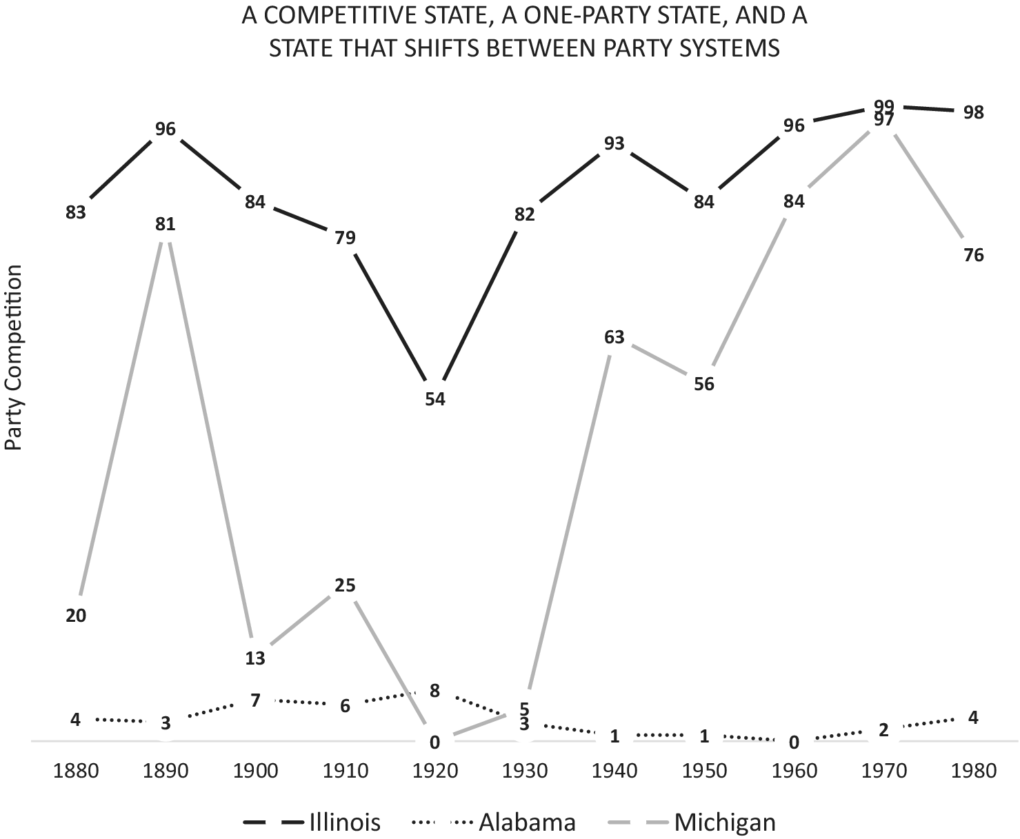
Figure 1. Levels of Party Competition over Time: Ideal Types, plus Michigan
If the whole world were Alabama and Illinois, we would have little causal leverage for this project. Our theory, of course, is that a two-party state like Illinois spends more on health care, education, and transportation—with better outcomes for its citizens in terms of health, literacy, and prosperity—than a one-party state like Alabama. But we have no convincing way to test that specific proposition in these two states because, alongside party competition, there exists a multitude of other factors, some measurable but many not, that distinguish Illinois from Alabama. To understand the impact of party competition, we must hold these other factors constant, and the best way to do that is to examine changes in party competitiveness over time within a given state. That is the basis of our research design: state fixed effects allow us to hold constant consistent differences across states and focus our analysis instead on the decade-to-decade variation in levels of party competition within states.
Michigan, as Figure 1 suggests, offers a path forward—and Michigan, not Alabama or Illinois, is representative of the great majority of states. In most states, the level of party competition ebbed and flowed between 1880 and 1980. Michigan provides a rich body of data for analysis, with party competitiveness fluctuating over time, between a low in 1920 of 0%—when both chambers in the legislature were entirely Republican—to a high of 97.3% in 1970, when Democrats controlled the house by a narrow 58–52 margin and the senate was equally split between the two parties. Figure 2 provides illustrations of some of the types represented by the American states. Some states, like Oregon and Pennsylvania, had competitive party systems in the late nineteenth century and in the second half of the twentieth century, but were dominated by one party in the early twentieth century. Others, like Kentucky and Maryland, were the mirror image, with competitiveness peaking in 1920. And still others, like Florida and Vermont, were one-party states, one Democratic and the other Republican, until the 1960s, when both became competitive. Over a century’s time, there are as many patterns of changes in party competition as there are American states—and it is this very variety, above all the changes from decade to decade within each state, that provides the foundation for the causal claims we investigate.
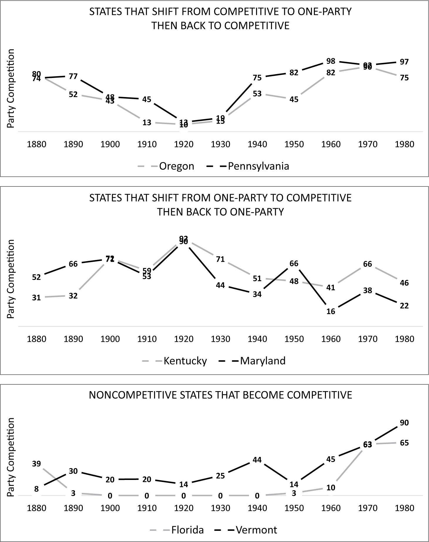
Figure 2. Levels of Party Competition over Time: Varied Patterns
We focus on party competition in the state legislature because that is where the collective spending and policy decisions that should directly affect state development take place. However, because executive branch officials also exert an important influence over policy, party competition for statewide offices may be an additional relevant measure. Using the dataset generously shared by Ansolabehere and Snyder (Reference Ansolabehere and Snyder2002), we compiled the average margin of victory in the contests for U.S. Senate, all U.S. House races, governor, and any other statewide offices held in a state in a given year. This is the same measure that Besley, Persson, and Sturm (Reference Besley, Persson and Sturm2010) use in their study examining the relationship between party competition and economic growth. We include this electoral measure alongside the legislative margin of competition to hold this factor constant and to see if it adds any additional explanatory power in our models.
Control Variables
Our hypotheses about the impact of party dynamics are ceteris paribus expectations. Yet because all is never equal in the American states, we include in our models a set of political, economic, and demographic control variables in order to isolate the effects of party competition.
Democratic Party Strength
Spending patterns may be more a function of which party controls a state rather than the level of two-party competition. While the literature probing the effects of state party control on spending has yielded mixed findings based on the era studied or the “party cleavage types” (Barrilleaux and Miller Reference Barrilleaux and Miller1988; Brown Reference Brown1995; Dawson and Robinson Reference Dawson and Robinson1963; Dye Reference Diamond1966; Hofferbert Reference Hofferbert1966; Schneider Reference Dye1988; Smith Reference Schneider1997; Winters Reference Mitchener and McLean1976), this is still an important alternative explanation for us to consider. To account for this, we construct measures of which party controlled the upper and lower houses in each legislature, based on the data reported by Dubin (Reference Dubin2007), to determine whether Democratic control led to higher spending. Since governors, too, are central in making state spending decisions (Caughey, Warshaw, and Xu Reference Caughey, Warshaw and Xu2017; Kousser and Phillips Reference Kousser and Phillips2012), we record the partisanship of the governor in each state in each decade and include this measure in our regression models.
Income per capita
A primary factor in determining a state’s ability to invest in governmental spending—as well as an important determinant of its rate of development, which we will discuss in the next section—is the economic resources of its residents. Indeed, state income has been a main variable in work in political science (Barrilleaux and Miller Reference Barrilleaux and Miller1988; Brown Reference Brown1995; Dawson and Robinson Reference Dawson and Robinson1963; Dye Reference Diamond1966; Hofferbert Reference Hofferbert1966; Schneider Reference Dye1988; Smith Reference Schneider1997; Winters Reference Mitchener and McLean1976) and in economics (Besley and Case Reference Besley and Case2003; Besley, Persson, and Sturm Reference Besley, Persson and Sturm2010; Frank Reference Frank2009; Mitchener and McLean Reference Smith2003) that have looked at state policy choices and growth rates. We expect that more affluent states will be able to spend more in all areas and that economic attainment may also condition future development. Our measure of per capita income comes from Klein (Reference Klein2009) for 1880–1910, from Lee et al. (Reference Lee1957, 753) for 1920, and from Bureau of Economic Analysis (2016) for 1930–2010. To convert this measure into current (2016) dollars, we rely on McCusker (Reference McCusker1991, 297–373) for data from 1880 to 1910 and on Federal Reserve Bank of Minneapolis (2021) thereafter.
Foreign-Born Percentage of State Population
A consistent finding of the literature on state and local politics in America is that jurisdictions with many immigrants face particular obstacles when it comes to obtaining funding or finding legislative success (Abrajano and Hajnal Reference Abrajano and Hajnal2015; Gamm and Kousser Reference Gamm and Kousser2013). Immigration has been a flashpoint throughout American history, with different national origin groups facing discrimination but the presence of discrimination remaining constant. To test for this, we use census data to measure the percentage of foreign-born residents in each state. For 1880 through 1990, this is reported in Carter et al. (Reference Carter, Gartner, Haines, Olmstead, Sutch and Wright2006). For 2000 and 2010, we use Grieco et al. (Reference Grieco, Trevelyan, Larsen, Acosta, Gambino, de la Cruz and Gryn2012).
Black Percentage of State Population
At least as much as immigrants have faced discrimination, Black Americans have long seen significantly lower spending levels on social services in the states in which they are most numerous (Grogan Reference Grogan1994; Plotnick and Winters Reference Plotnick and Winters1985). To control for this factor, we use the census figures in Carter et al. (Reference Carter, Gartner, Haines, Olmstead, Sutch and Wright2006) before 2000 and in Rastogi et al. (Reference Rastogi, Johnson, Hoeffel and Drewery2011) thereafter.
Other Nonwhite Percentage of State Population
Because ethnicity along with race has been a source of discrimination in the United States, we also measure the “other nonwhite” population in the state—a census category that, depending on the year, includes Asian American, Native American, Latino/a/x, and Hawaiian and Pacific Islander residents. Hajnal and Trounstine (Reference Hajnal and Trounstine2005) offer evidence of ethnic and racial biases in local spending, and Hero and Tolbert (Reference Hero and Tolbert1996), Hero (Reference Hero1998), Filindra and Pearson-Merkowitz (Reference Filindra and Pearson-Merkowitz2013), Butler (Reference Butler2014), and Harden (Reference Harden2015) show how policy makers discriminate against ethnic minorities at the state level. We gather these figures from Carter et al. (Reference Carter, Gartner, Haines, Olmstead, Sutch and Wright2006) before 2000 and in Hoeffel et al. (Reference Hoeffel, Rastogi, Kim and Shahid2012), Hixson, Hepler, and Kim (Reference Hixson, Hepler and Kim2012), and Norris, Vines, and Hoeffel (Reference Norris, Vines and Hoeffel2012) afterward.
Urban Percentage of State Population
Finally, states with dense urban populations, compared with those with a larger percentage of rural residents, face different demands for the scope of government and the types of services that the state is called upon to provide. States with more city dwellers may also have a different capacity to develop quickly. To control for the effect of the urban share of the population, we collect demographic figures from Carter et al. (Reference Carter, Gartner, Haines, Olmstead, Sutch and Wright2006) for all years through 1990, from the State Data Center of Iowa (2000) for 2000, and from the U.S. Census Bureau (2010) for 2010.
State Spending
How much each state spends—and in what areas—is a pivotal variable in this study. For our first set of models, state spending functions as the dependent variable, as we test the hypothesis that party competition affects the amount and allocation of dollars. And, for the second set of models, state spending becomes the crucial independent variable, as we ask whether expenditures on human capital and transportation infrastructure affect the well-being of people living in the state.
We rely on two main sources of data. Our primary source is a series of reports issued by the U.S. government aggregating local and state expenditures for each state, with figures for total spending as well as figures for spending by subject area. These reports—which cover state and local spending in 1902, 1913, 1932, 1942, 1962, 1972, and 1982—were aggregated by Sylla, Legler, and Wallis (Reference Sylla, Legler and Wallis1995) into a single database, which we draw on for our analysis. To extend this time series back to the nineteenth century, Sylla, Legler, and Wallis (Reference Sylla, Legler and Wallis1993) scoured archives and libraries to collect budget records reported at the state level. The resulting data series is less comprehensive than the one created by the federal government, with some obvious gaps in state coverage and no data on local spending. Still, given that spending figures in the two data series are strongly correlated during the period they overlap in the early twentieth century and given, too, that no other comprehensive record exists for this era, we rely on this second database for state spending in 1880 and 1890. Most of our analysis, however, relies simply on the twentieth-century spending data.
Our theory links expenditures to party competition at the state level and to decisions of state legislators, but local governments have historically played powerful roles in allocating money for public goods, especially in the realm of education but also in such areas as sanitation, transportation, and public safety—and states differ considerably on this dimension (Bloom Reference Bloom2019; Burns Reference Burns1994; Teaford Reference Teaford1984; Reference Teaford2002). Comparing statewide investments requires, then, that we aggregate, as much as possible, expenditures made at both the state and local levels. That is consistent with the practice in these federal reports. This approach is appropriate because, in the American system, state and local governments are not separate layers of government but intertwined entities, with states exercising authority over local governments through the judicial precedent of Dillon’s Rule and with many states heavily funding local governments. While power and spending are devolved in different ways in different states, the federal reports account for this by aggregating total state and local spending.
These reports include money from federal transfers to state and local governments alongside own-source revenues as the funding that supports total expenditures. Since federal transfers are often not segregated in the ways that they are spent, including these dollars is necessary (and, given the nature of state spending, unavoidable) if we are to provide a comprehensive picture of a state’s investment in infrastructure and human capital. However, we need to attend to the concern that these federal transfers might be substantial in scale and correlated with levels of party competition in the state legislature. While we have no theory that would predict that federal transfers are related to a state’s partisan competitiveness, if the two variables were to be positively correlated, we could not rule out the alternate hypothesis that federal transfers, rather than two-party competition, are driving investments in education, health care, and transportation. The federal government began reporting data on federal transfers in its 1942 report—between 1880 and 1932, before the New Deal, federal transfers to state and local governments were quite small—so we did a special analysis of the data from the 1942, 1962, 1972, and 1982 reports. We find that, even in the most recent decades, states still draw on own-source revenues for the vast majority of their spendingFootnote 1 and that there is no correlation between the level of federal aid to each state and its level of party competition.Footnote 2 This finding alleviates any concern that competitive legislatures are investing more in education, health, and transportation simply because they have more federal money to spend.
As Figure 3 shows, spending on education, health care, and transportation have generally risen over time, in constant dollars, across all states. These parallel trends satisfy a foundational requirement of the difference-in-differences technique. Just as important, though, is the substantial variation among the states. We offer three sets of examples in Figure 3. On education spending, Idaho consistently spent more than Delaware from 1900 until 1940—though the lines on the graph are compressed, the differences, such as $173 versus $52 in 1910, were very large—then, in 1940, the lines crossed. Since then, Delaware has been the bigger spender on education, though the two states came close to converging again in 1980 after a large drop in spending in Delaware. On health spending, Figure 3 shows two states, Indiana and Minnesota, with nearly identical levels of spending from 1900 to 1960, which then diverge sharply in 1970 and 1980. And Georgia and Maine, which we illustrate for transportation spending, began at the same level, but diverged early. By 1930, Maine spent more than four times as much as Georgia on transportation, and Maine continued to outpace Georgia in this realm by a considerable amount until 1980, when Maine’s spending fell sharply, in constant dollars.
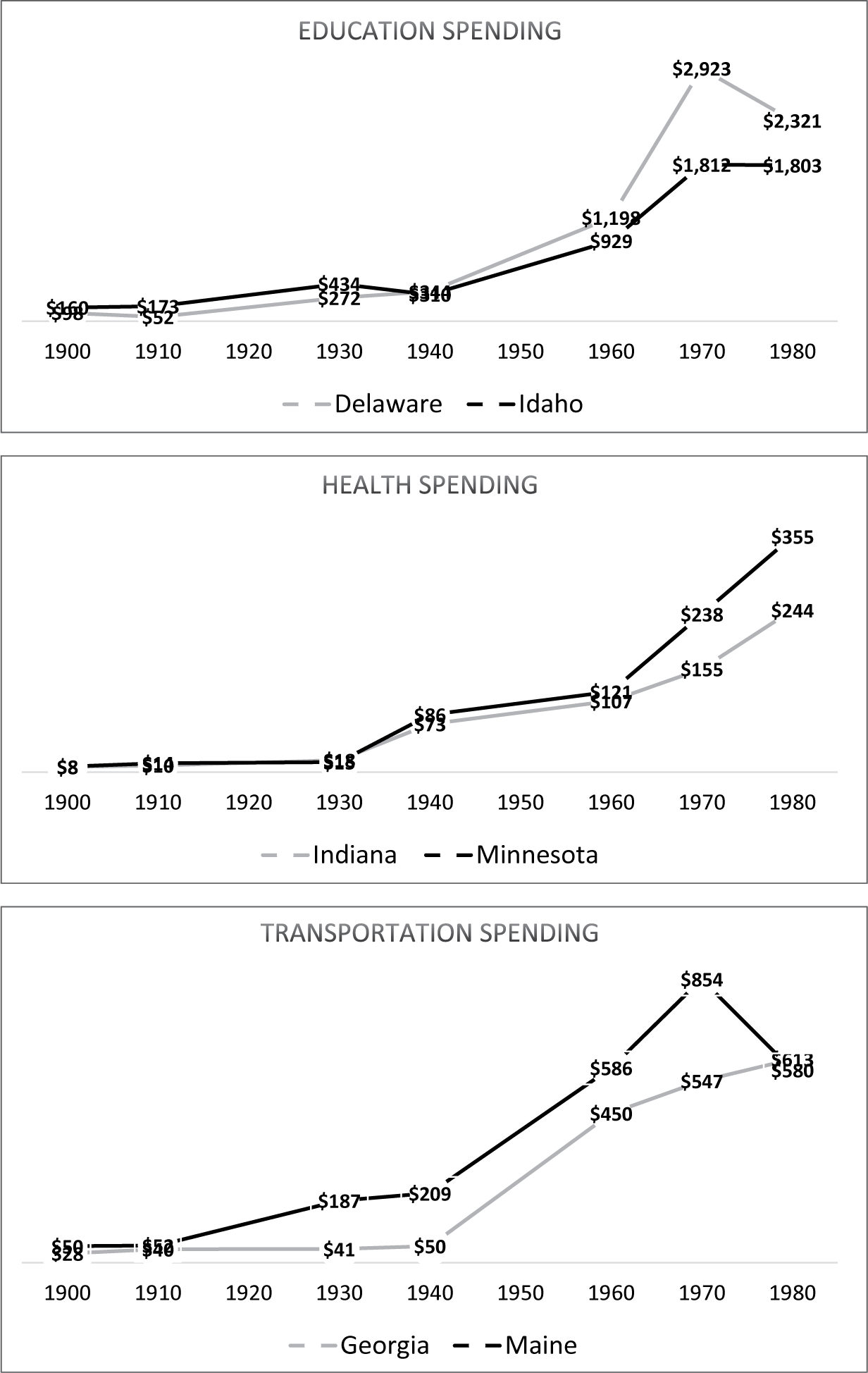
Figure 3. Education, Health, and Transportation Spending (in Per Capita, Constant Dollars)
This decade-by-decade variation, replicated across all the states, is crucial for our study. Coupled with variation in levels of party competition, it allows us, first, to perform within-state analysis of the influence of changes in party competitiveness on state spending decisions. And, second, that same variation allows us to engage in within-state analysis of how changes in spending affect the well-being of state residents.
Measures of Health, Education, and Income
Identifying measures for wellness outcomes, especially at the state level and over a century’s time, was a wide-ranging research challenge. To our knowledge, no comparable dataset has been assembled before. We drew on an array of sources, identified in the Data Sources document posted in the American Political Science Review Dataverse, and consulted other scholars to construct datasets that document residents’ well-being in these states at 10-year intervals between 1880 and 2010. For this article, we only present data in which we have great confidence: where we could not resolve significant historical problems or doubts, we do not use those data. For each variable (except high school graduation rates, which we explain below), all the data come from a consistent set of sources and, in any given year, the data for every state is drawn from exactly the same source.
Figure 4 summarizes our five primary wellness measures, with each state in each decade represented as a dot. The broad trend lines are clear: on all five wellness measures, the state of the American population has improved over time. Infant mortality and illiteracy have fallen, while life expectancy, graduation rates, and income have all risen over the last century. As was the case with state spending, the patterns apparent in this figure provide support for a key assumption of the difference-in-differences models: the assumption of parallel trends. What Figure 4 conceals, though, is state-by-state variation and year-by-year changes in individual states. Our within-state analysis requires that, just as changes in party competition and spending vary from state to state, the same variation be present in this set of dependent variables. We proceed, then, to present figures on measures of well-being that focus on one measure at a time, allowing us to isolate individual states and to compare changes in one state to those in another.
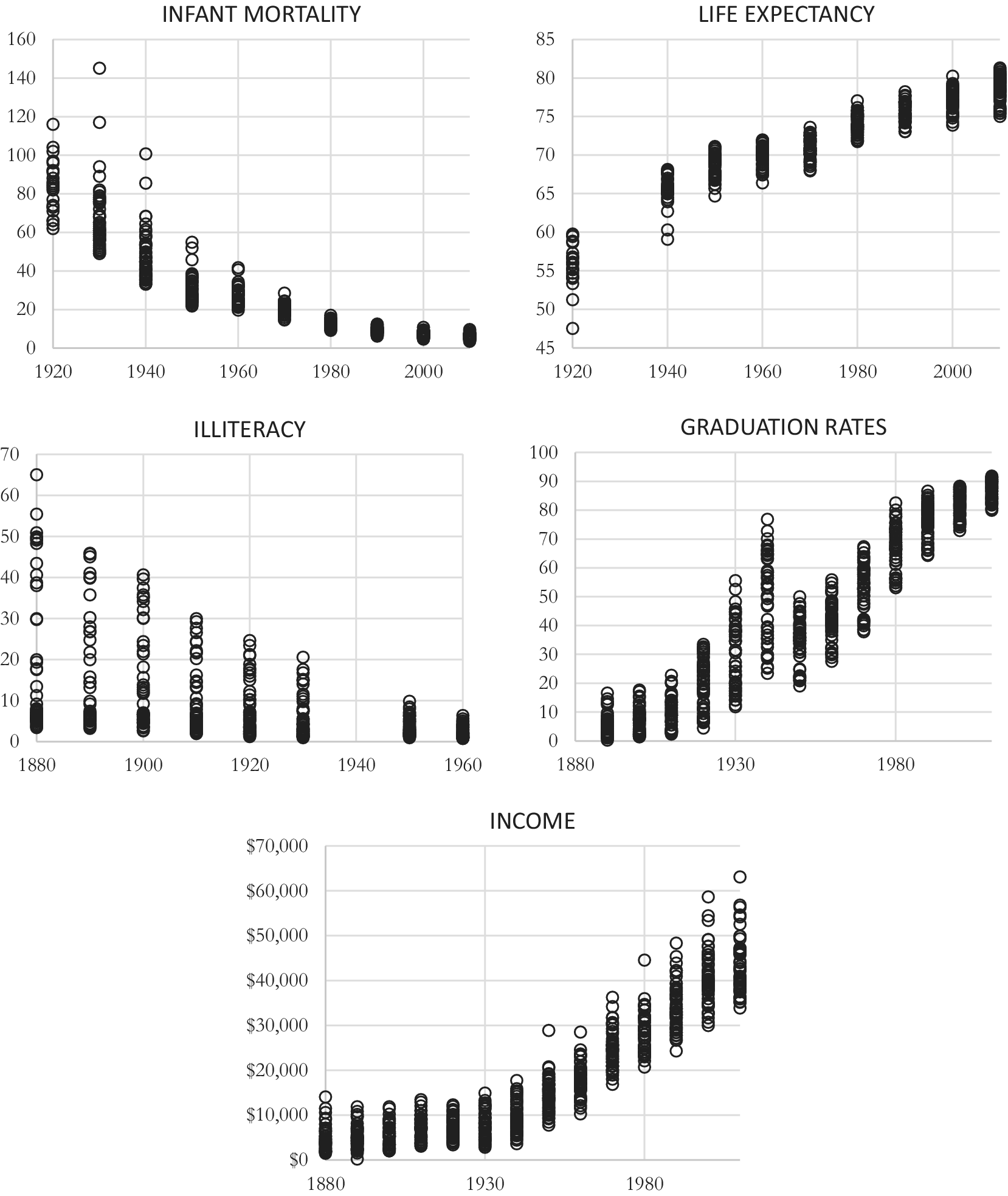
Figure 4. Measures of Life, Literacy, and Prosperity over Time in 50 States
Life—Infant Mortality
While the federal census reported figures on infant mortality beginning in 1890, not until 1910 did it begin reporting data only for “registration states,” where federal officials trusted the state data. The number of registration states increased from seven in 1910, to 23 in 1920, to 46 in 1930, and to all 48 in 1933. Figure 5 illustrates infant mortality rates (where data exist) over the period 1920–2010. Each state is represented by a gray line in the figure, with the lines of two states highlighted. As this figure shows, there was historically great variation in levels of infant mortality and in the rate of improvement. Mississippi and New Mexico, for example, dramatically reversed positions over time. In 1930 the infant mortality rate in Mississippi, 68 deaths for every 1,000 live births, ranked it somewhere in the middle of states. But by 1960, Mississippi’s rate, at 42, was the highest in the country, and it has been the highest ever since, even as it has continued to decline. New Mexico, in contrast, which in 1930 had by far the highest rate in the country with 145 infant deaths for every 1,000 live births, now ranks in the middle of the pack. Rates in all states have fallen and converged over the last few decades, but there remain significant differences between states. Mississippi’s rate in 2010, 9.6 deaths per thousand, is 70% higher than New Mexico’s, at 5.6.
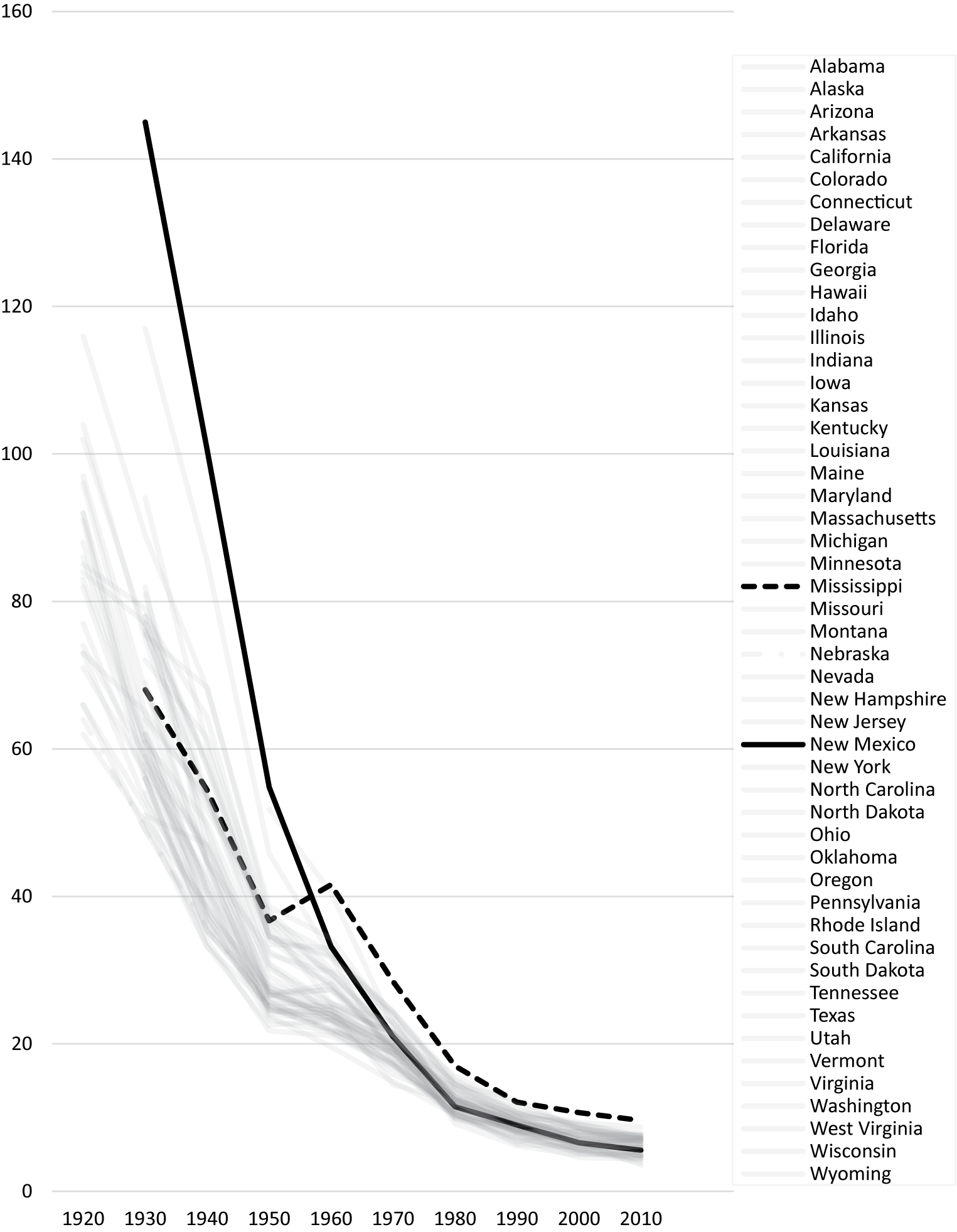
Figure 5. Infant Mortality
Life—Life Expectancy at Birth
The federal census reported life expectancy data for just one state (Massachusetts) in 1890, five states in 1900 and 1910, and half the states in 1920. The 1920 and 1940 state-level data were reported only for whites, and there was no 1930 data at all.Footnote 3 Only in 1950 did the federal census begin systematically reporting life expectancy for all people in each state. Examining Figure 6, the general trend is clear: steady improvements in life expectancy at birth. But differences between states have been substantial. In 1920, life expectancy in the territory of Hawaii was just 47.5 years, the lowest in the country, and in California it was 55.8 years. By 1960, with full data reported for all states, Hawaii’s rate, at 71.6, slightly exceeded California’s, at 70.8. In subsequent decades, Hawaii—which had once had the lowest life expectancy in the country—has had the highest. California, which lagged behind Hawaii in the second half of the twentieth century, nearly closed the gap by 2010. The variation among the states is evident throughout the whole time period, including the period since 1950 when the fullest data are available.
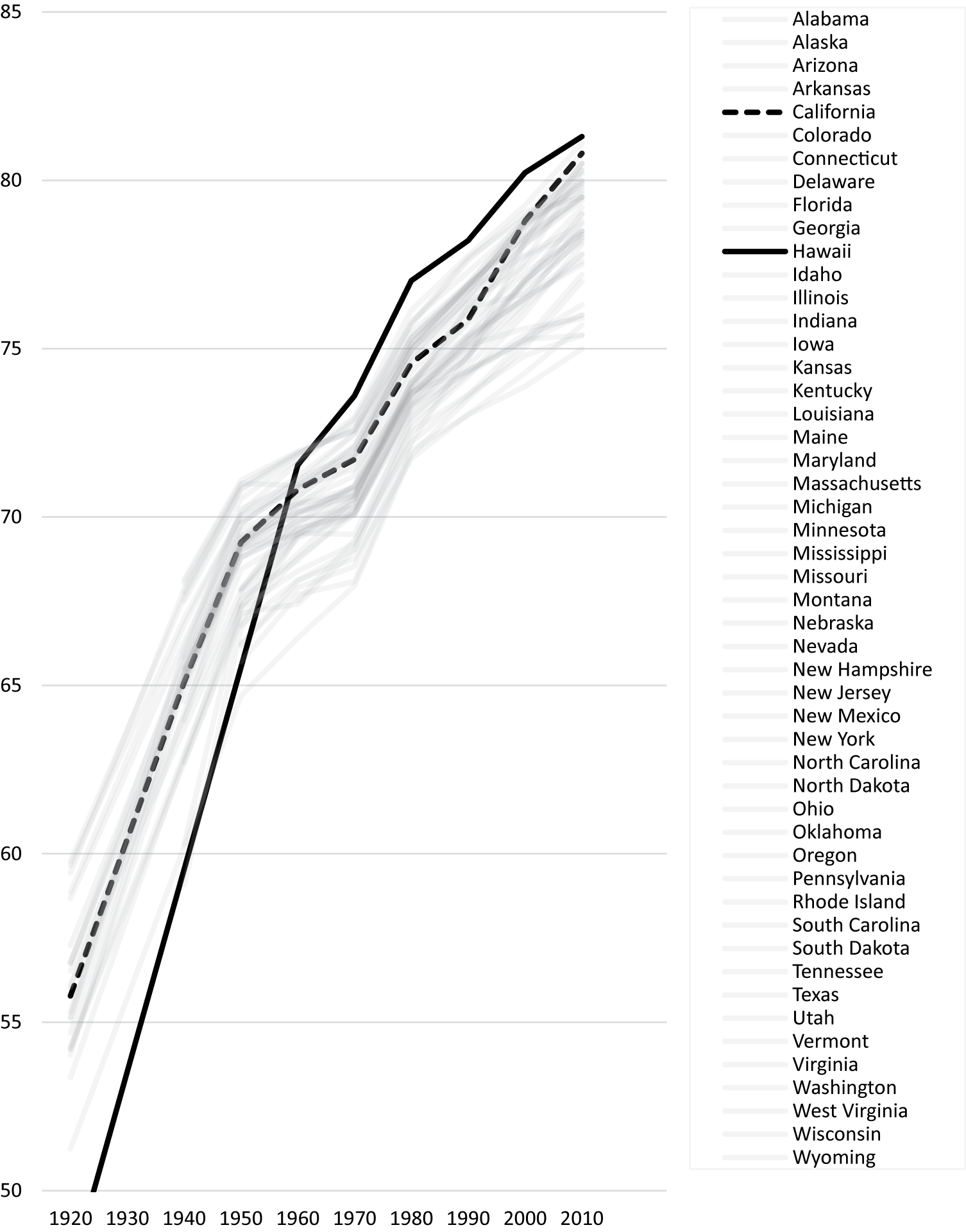
Figure 6. Life Expectancy
Literacy—Illiteracy Rates
Between 1880 and 1960, when the data series ends, the federal census reported illiteracy rates for each state’s population. As Figure 7 suggests, state populations once differed dramatically on this measure. In some states, like Virginia, the rate has plummeted over time—from 40.6% (1880) to 24.3% (1900) to 3.4% (1960). In others, like New York, illiteracy rates were already low, at 5.5% in 1880 and decreased only slightly over time, to 2.9% in 1960—a small decline next to the experience in Virginia, but still a considerable improvement from the perspective of New Yorkers.
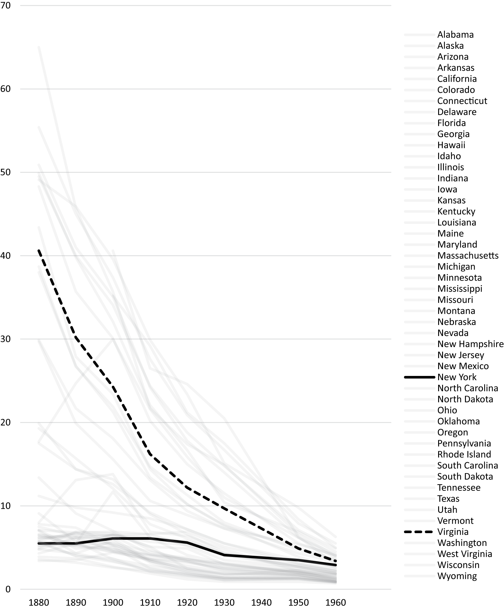
Figure 7. Illiteracy Rate
Literacy—High School Graduation Rates
To measure high school graduation rates, we draw on two different data series. For the period 1890–1940, our data estimate the proportion of 18-year-olds who graduated in a given year from high school. For the period 1950–2010, our data show the proportion of all adults who are high school graduates. In an age when high school graduation rates steadily increased—which by definition means that the proportion of young adults with high school degrees is greater than the proportion of older adults with high school degrees—the first measure is markedly higher. Both data series, separated by a gap, are illustrated in Figure 8.
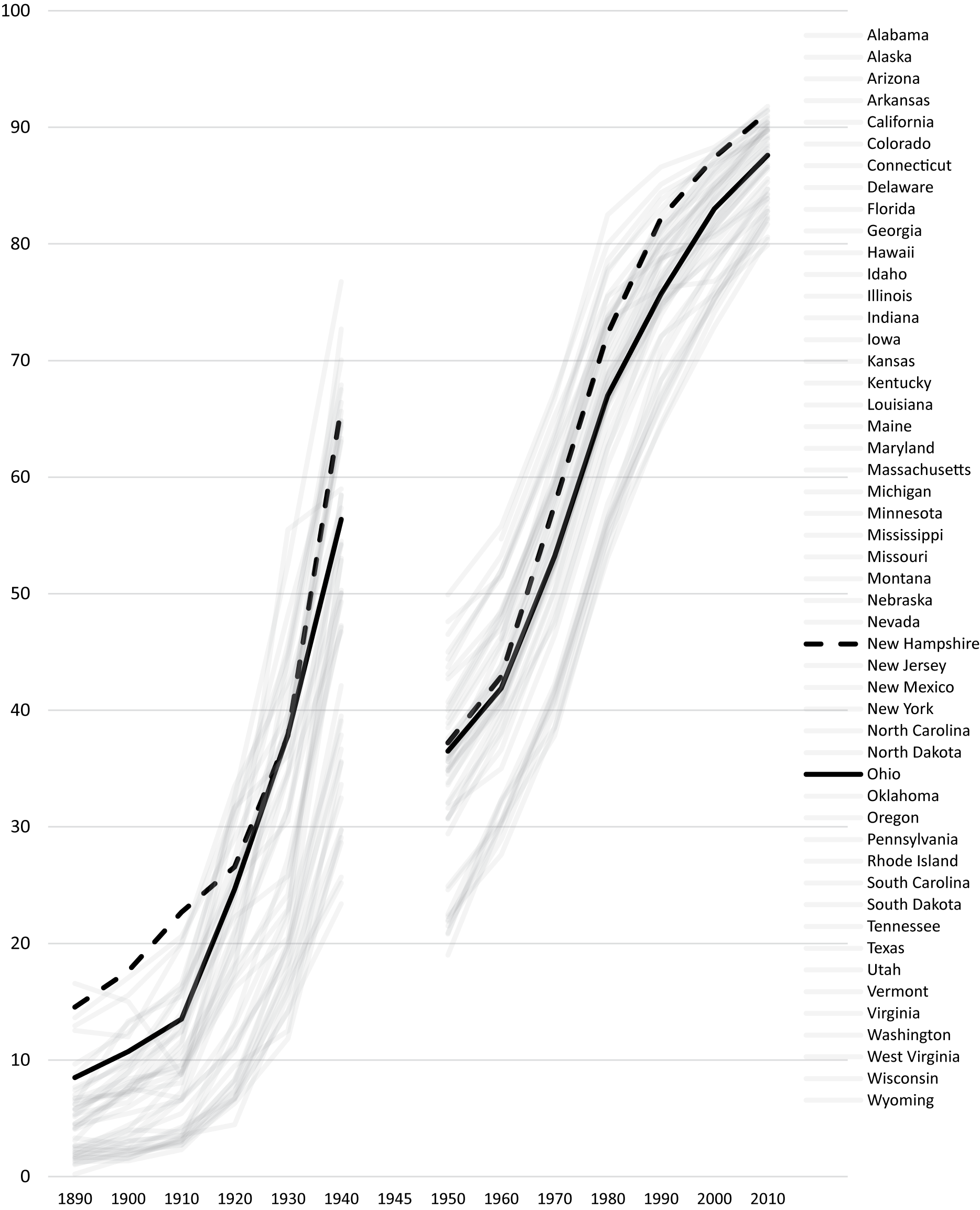
Figure 8. High School Graduation Rates
Before 1940, the federal government did not collect data on the number of high school graduates in each state’s adult population. So we instead report an estimated number of each year’s high school graduates, as a proportion of that state’s 18-year-olds. (In calculating this estimate, we draw extensively on Goldin Reference Goldin1994 as well as on a number of primary sources. See our Data Sources document posted in the American Political Science Review Dataverse for a detailed discussion.) As Figure 8 indicates, these data show great improvement over the period 1890–1940, with all states trending sharply up. But states, on this as on other measures, varied. Ohio, which had a lower graduation rate than New Hampshire at the turn of the twentieth century—with Ohio at 10.7% in 1900 and New Hampshire at 17.6%—had risen to 37.9% by 1930, with New Hampshire at 37.8% that year.
Since the middle of the twentieth century, data on graduation rates is straightforward to locate: the federal government has regularly surveyed the population and reported the percentage of adults in each state who graduated from high school. These are the data we report for 1950–2010. The story here, again, is of progress across the board, but each state charted its own path. Starting by this measure at the same place in 1950, at 37%, New Hampshire and Ohio followed different trajectories over the next 60 years. New Hampshire, which at the turn of the twentieth century had more teenagers graduating from high school than Ohio, had more high school graduates in its population at the turn of the twenty-first century. In 2010, 91.3% of New Hampshire’s adults and 87.6% of Ohio’s adults had graduated from high school.
Prosperity—Income per capita
The final measure of well-being, income per capita, is drawn from the same data sources identified in the previous section. In the first stage of our analysis, we use present income as a variable to predict the level of state spending, given our expectation that states with the capacity to raise more in tax revenue are likely to spend more than other states. But, in the second stage of our analysis, we use future income as a measure of a state’s success in stimulating greater prosperity after investments in human capital and infrastructure have time to pay off. Using per capita income as a measure of economic growth follows the approach of other historical works on political economy in the states, since state GDP data are not available before the 1960s (Barro and Sala-i-Martin Reference Barro and Sala-i-Martin2004; Besley, Persson, and Sturm Reference Besley, Persson and Sturm2010). Figure 9 offers an example of the disparities among states on this measure. Measured in current (2016) dollars, per capita income in Connecticut, already relatively high at $6,300 in 1880, rose to $63,000 by 2010, higher than that of any other state. Montana, in contrast, buoyed by silver and copper mining in the late nineteenth century, began at a very high level—$10,600 in 1880—but rose to just $38,000 by 2010.
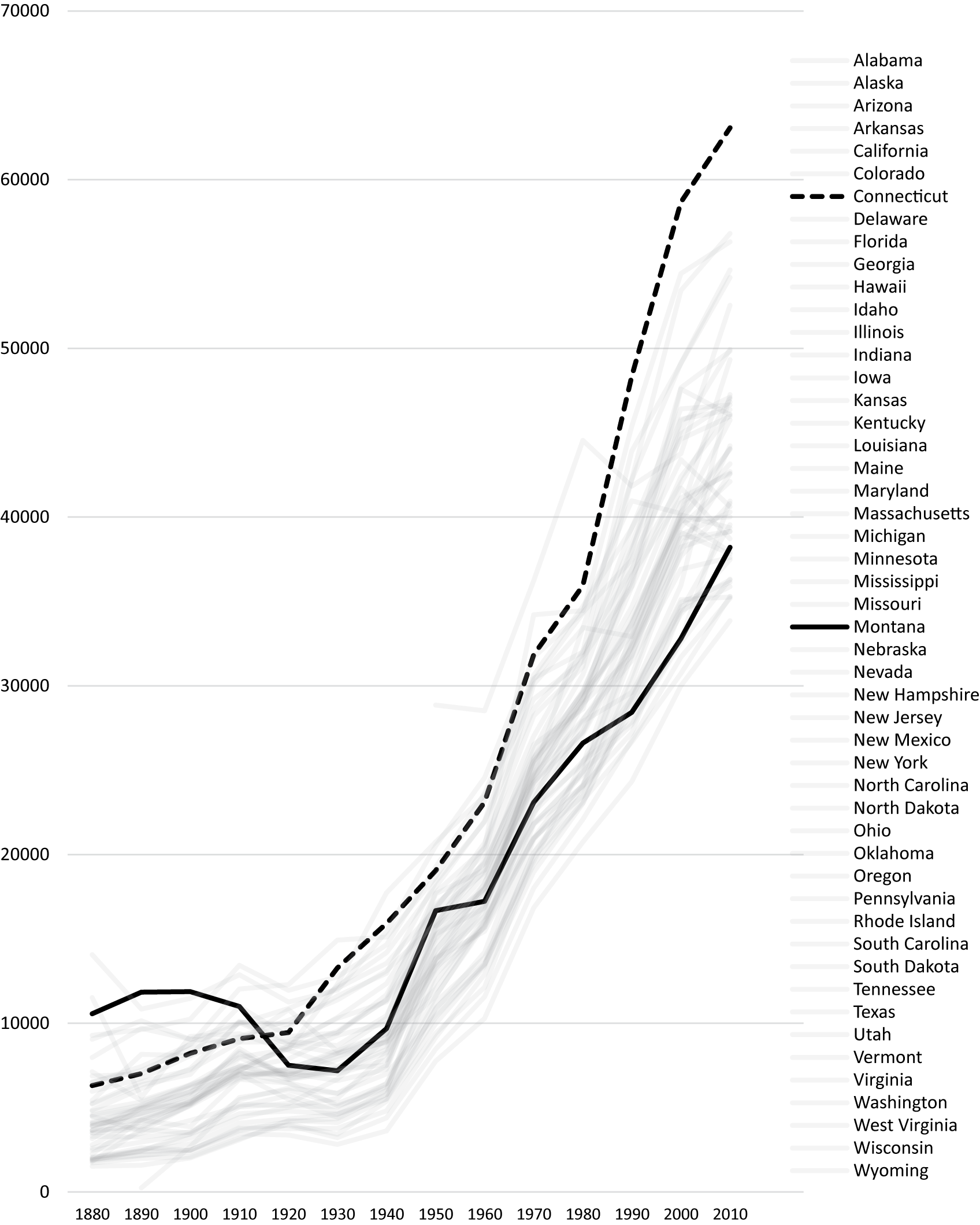
Figure 9. Income Per Capita
DOES PARTY COMPETITION SHAPE SPENDING PATTERNS?
Our first empirical question probes the initial link in our causal chain, asking whether party competition gives lawmakers the motivation and the means to pass the major statewide programs that lead to larger investments in human capital and infrastructure. If so, we should observe higher spending levels in the three areas that specifically respond to broad public demands and potentially facilitate development: education, health care, and transportation. In order to further strengthen our research design, we also conduct a series of placebo tests showing that closely competitive states invest in these three areas but that they do not spend more in other budget areas such as public safety, social services, and other governmental functions.
To isolate the impact of party competition on spending patterns, we turn to time-series, cross-sectional models with state and year fixed effects. The difference-in-differences models reported in Table 1 explore the effects of changes over time within a state. Our models ask whether, in a year in which party competition is particularly high, a state spends more than its expected baseline level. Year fixed effects account for the national trends that affect all states at the same time, such as macroeconomic fluctuations, changes in federal aid, and new demands on the role of government. State fixed effects give each state its own baseline, alleviating the concern that there is some omitted characteristic that leads a state to have a one-party system and, independently, to spend less and develop more slowly. This sort of endogeneity would threaten a cross-sectional research design, but our approach controls for consistent state-to-state differences. A state’s status as one-party or competitive appears to have been driven by major, exogenous events, such as the Civil War, Reconstruction, the 1896 realignment, the New Deal, or the civil rights revolution of the 1960s—and it was rarely fixed.Footnote 4
Table 1. Party Competition Predicts Higher Human Capital and Infrastructure Spending, 1880–1980
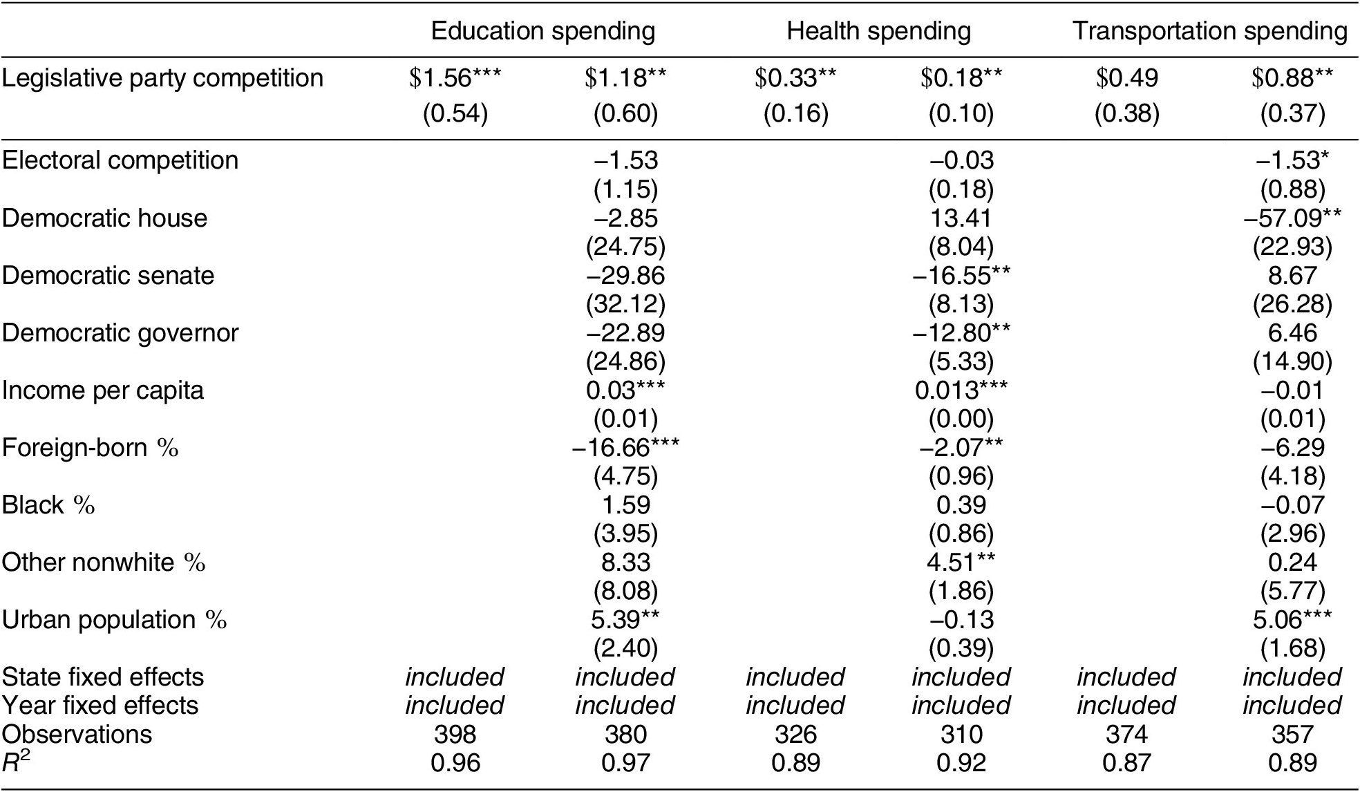
Note: Table entries are regression coefficients, with standard errors clustered by state in parentheses. ***p < 0.01, **p < 0.05, *p < 0.10 in a one-tailed test.
Our first models examine the influence of party competition on spending in each area with only these two fixed effects, to ensure that the effect is clear and does not depend on the mixture of other variables used in the model. Our second models include a full set of political, economic, and demographic controls, to account for the fact that states experience different shifts in these characteristics over time which may covary with party competition.
Using both approaches, we observe the strong influence of legislative party competition on investment in human capital and transportation infrastructure. All of these effects are statistically significant at the 95% confidence level. In our models of education spending, party competition has a strong and significant impact upon spending whether or not we also include control variables. Every additional percentage point in competitiveness leads, in the model with the full host of controls, to a predicted $1.18 increase in education spending. A shift in party competitiveness between that in Michigan in 1920, when Republicans held every seat in the legislature, and an evenly balanced legislature, which Michigan approached in 1970, brings a 100-point increase in party competition and thus a predicted $118 increase in spending per capita. Since education spending per capita averages $699 across the span of our dataset, the effect of party competition on it is substantively as well as statistically significant.
Party competition also exerts significant impacts on spending on health and sanitation and on investment in transportation infrastructure. In the model with political, economic, and demographic controls, a full 100-point increase in competition would bring a predicted $18 increase in spending on health (which averages $103 per capita in this period). For transportation, the same increase in competition would yield $88 more in per capita spending (in a policy realm that averages $276 per capita in each state). Note that these estimates come from models that hold constant which party controls the governorship and each house of the state legislature, along with the level of competition in statewide elections, income levels in a state, immigrant and nonwhite percentages of the population, and the urban population share. The fact that party competition exerts large and consistent effects, while holding so much else equal, highlights its critical influence.
While we find strong evidence that legislative party competition appears to drive increases in spending on health, education, and transportation, one concern is that competition may simply drive up state spending in every policy domain. To address this, we run the placebo tests reported in Supplementary Table A.1, available in our Supplementary Materials. These estimate the influence of party competition on the other major areas of state spending. According to the theory that close party competition incentivizes specific investment in developing human capital and infrastructure, but not spending in other realms, we should find null effects on other areas of spending. This is generally what we observe. Party competition has no effect on public safety spending or the residual “other spending” category (which is the second largest category), and there is suggestive evidence that it actually leads to a decrease in social service spending. Overall, what these placebo tests show is that two-party states do not spend more in every area but instead invest specifically in human capital and infrastructure.
Beyond party competition, the coefficients reported in Tables 1 and A.1 highlight what is held constant in these analyses and report observed effects. The strongest finding, and one that is consistent with a plethora of prior studies, is that spending rises when per capita incomes are higher; this is true even with state and year fixed effects. Spending in most areas is also lower when the foreign-born percentage in a state is particularly high, consistent with findings by Gamm and Kousser (Reference Gamm and Kousser2013) and Abrajano and Hajnal (Reference Abrajano and Hajnal2015). Spending on education, transportation, and the “other government areas” category is higher when urban population percentages rise. Perhaps most surprising to contemporary readers, Democratic Party control of the legislature and the governorship yields only a few mixed effects. Yet the lack of an effect of party control on spending mirrors studies from an earlier era (Dawson and Robinson Reference Dawson and Robinson1963; Dye Reference Acemoglu, Naidu, Restrepo and Robinson1966; Hofferbert Reference Hofferbert1966; Winters Reference Mitchener and McLean1976). It also fits with Caughey, Warshaw, and Xu’s (Reference Caughey, Warshaw and Xu2017) finding that while the election of Democrats has led to more liberal policies since 1980, the link between party control and policy liberalism was much weaker throughout the earlier period studied in our regressions.
As a check on the robustness of our findings, we investigate whether the link between party competition and spending patterns was present even before the myriad changes that took place in state governments beginning in the 1960s. Ansolabehere, Gerber, and Snyder (Reference Ansolabehere, Gerber and Snyder2002) show that the reapportionment revolution following the Baker v. Carr decision in 1962 shifted spending patterns across types of districts, while changes in state tax policies (Teaford Reference Teaford2002), increasing federal grants to states (Bloom Reference Bloom2019), and the movement to professionalize state legislatures accelerated in the late 1960s and onward. To ensure that changes occurring after 1960 are not driving our results, in Supplementary Table A.2 we reestimate these models with data only for the period 1880–1960. We find that the influence of party competition on education spending and on health spending remains strong and significant. The effect of competition on transportation spending loses its statistical significance in these models that draw on fewer observations, but the estimated effect is still positive. This analysis shows that our effects are not time bound or a function of the redistricting revolution or other changes in the 1960s.
DO STATE INVESTMENTS PAY OFF IN WELL-BEING?
Do the decisions that parties make in state capitols change the lives of their state’s residents? This is a threshold question to evaluate whether the strong links that we find between party competition and spending patterns have implications for the long-term arc of development in the American states. In this section, we test the impact of investments in human capital and infrastructure on state health, educational, and economic outcomes.
As we did in our analysis of spending patterns, we take a difference-in-differences approach. This maximizes the causal leverage that we can draw from our time-series, cross-sectional data by using state and year fixed effects, alongside a set of economic and demographic controls, to hold constant the unmeasured characteristics of each state and the common national forces that might affect development in all states in a given decade. Our models explore the impact of changes in spending levels on development over time within a state, relative to its expected baseline level.
We match the type of investment with the realm in which it could pay off. Thus we look at how health and sanitation spending affects infant mortality and life expectancy, at how education spending reduces illiteracy or increases high school graduation rates, and how health, education, and transportation spending influence income levels. We expect spending to have a nearly immediate impact in two of these realms: infant mortality and high school completion, because delivering more programs to these targeted populations could potentially change their outcomes in the short run. Average life expectancy, the percentage of the adult population that is illiterate, and overall per capita incomes are all population characteristics that should take longer to change, so we test for these policy effects one generation (30 years) later.
Table 2 reports the effects of spending on our life and literacy measures. We find that when states make strong investments in health care and education, these are generally followed by rapid progress in development. First, we find strongly significant evidence for our expectation that spending in health and sanitation reduces infant mortality rates. When a state spends an additional $18 per capita in this realm—which was the predicted effect on spending when moving from a one-party to a highly competitive legislature—it should see a decrease of 0.7 deaths per thousand births. This effect is significant at the 95% confidence level. Our models of life expectancy provide less conclusive evidence. Here, the impact of spending is significant only at the 90% confidence level in a one-tailed test.
Table 2. Spending Levels Predict Development, 1880–2010
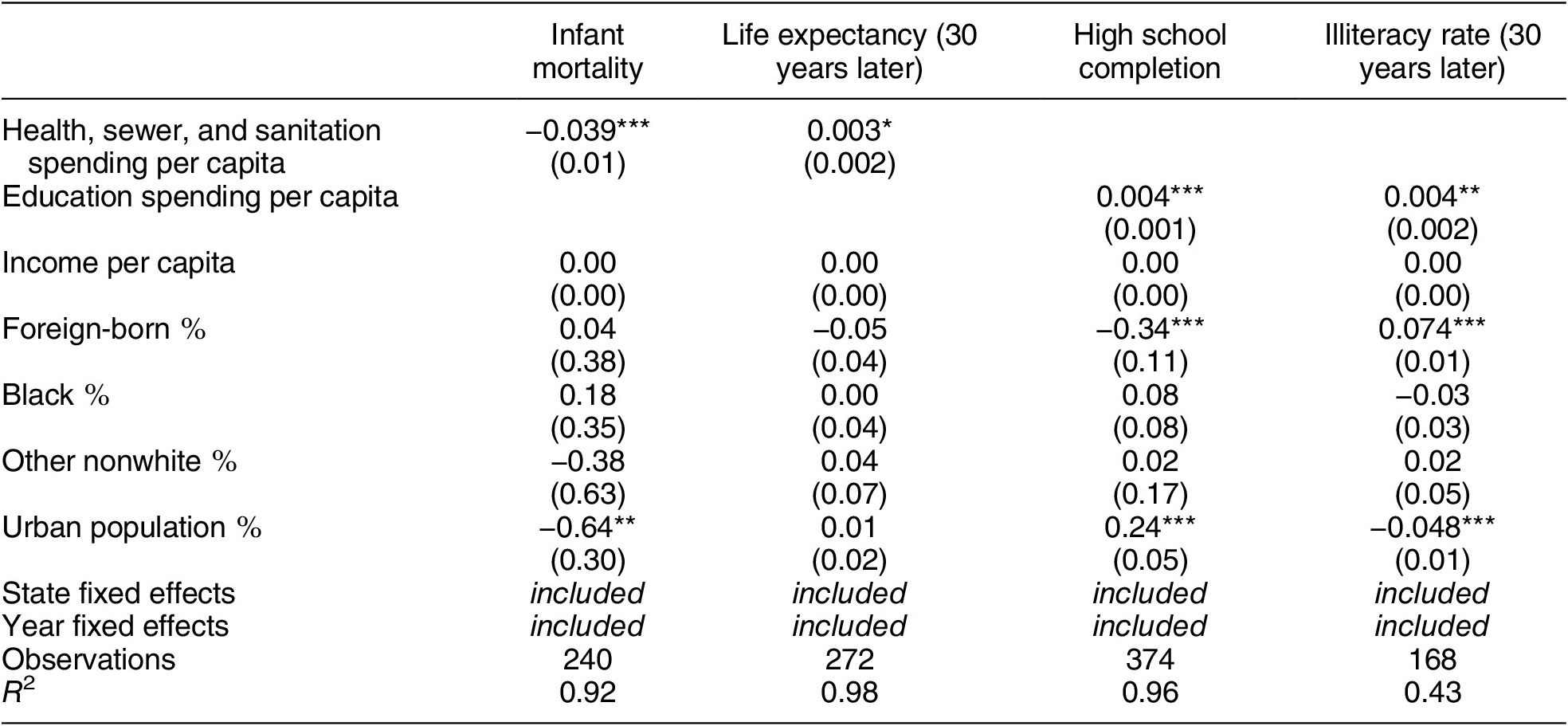
Note: Table entries are regression coefficients, with standard errors clustered by state in parentheses. ***p < 0.01, **p < 0.05, *p < 0.10 in a one-tailed test.
For education spending, both of our models reveal clear effects on development that are significant at 95% confidence levels and substantively important. Remember that our spending models in the prior section predicted that states with closely competitive party margins would invest $118 more per capita in this realm than those dominated by a single party. Our model of high school graduation ratesFootnote 5 shows that such an investment should increase graduation rates, measured immediately afterward, by half a percentage point. For illiteracy rates, measured 30 years later, such an investment would reduce the illiterate proportion of the overall population by nearly half a percentage point toward zero. Note that each of these effects is estimated within a state for a single decade: the accumulated effects of consistent investment over many decades can set states on very different developmental paths.
Table 3 reports the impact of spending—on health, education, and transportation—on our fifth measure of development, state income per capita. The three “full sample” models, estimated on data from our entire time series, do not show significant effects for any type of spending: the estimated impact of health, education, and transportation spending is always smaller than its standard error. Yet this overall null effect obscures an important time-bound effect in our dataset. When we look at the impact of spending during the pre–World War II period of our study—the state budgets passed from 1880 through 1940—we find that health and education expenditures had a strong positive effect on incomes. An additional $18 of health and sanitation spending leads to a predicted $257 increase in income levels 30 years later. When states spent an additional $118 on their education budgets, they could expect income levels to increase an extra $544 a generation later. Both of these effects are significant at the 95% confidence level. Transportation investment did not lead to any apparent payoff.
Table 3. Health and Education Spending Levels Predict Income (Only in Pre–New Deal Period)
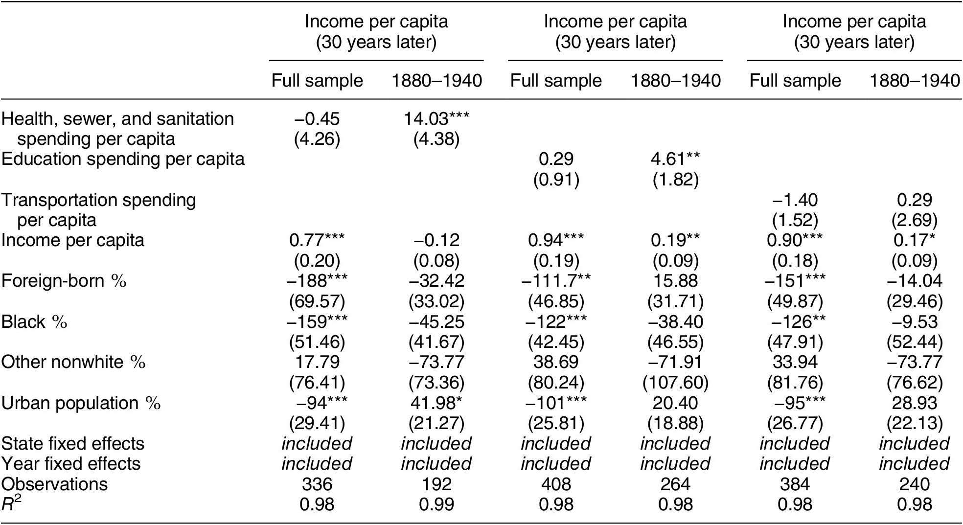
Note: Table entries are regression coefficients, with standard errors clustered by state in parentheses. ***p < 0.01, **p < 0.05, *p < 0.10 in a one-tailed test.
We did not have an a priori expectation that the impact of investment in human capital and infrastructure on incomes would only be present in decades through 1940. Post hoc explanations such as the New Deal, the economic boon that followed World War II, or the increased role that the federal government took in alleviating income disparities through Great Society programs could be advanced and explored in future work. Still, we think that the link between human capital spending and income growth over a six-decade period is an important feature of state politics worth noting.
CONCLUSION
When Schattschneider (Reference Schattschneider1942, 1) wrote that “modern democracy is unthinkable save in terms of the parties,” he expressed a sentiment that came to define the modern study of democratic regimes. That he wrote of “parties” rather than “party” was no accident; a single party was insufficient. Without competitive parties, voters lacked the ability to influence government through elections (Aldrich and Griffin Reference Aldrich and Griffin2018; but see Achen and Bartels Reference Achen and Bartels2016). “The grand objective of the haves is obstruction,” Key (Reference Key1949, 307) argued, based on his observation of the one-party American South in the 1940s. “Organization is not always necessary to obstruct; it is essential, however, for the promotion of a sustained program in behalf of the have-nots.”
With this article, we argue that party competition has been crucial to the well-being of the American people. Our findings buttress the argument that party competition leads legislators to spend more and to do so specifically by investing in human capital and infrastructure through expenditures on education, health and sanitation, and transportation. This spending then leads, in the short term and a generation later, to measurable improvements to the public welfare. We find that states that spend more—and spend more because of party competition—become places where children are more likely to survive infancy, where they learn to read and where they graduate from high school, where adults live longer lives, and, at least in the pre-New Deal era, where people earn higher incomes.
Our approach draws on work in comparative politics that examines the role of democratic institutions in promoting capital growth and well-being around the world. Building from Meltzer and Richard’s (Reference Meltzer and Richard1981) model, these works examine whether the transition from autocracy to democracy and expansion of the franchise empower poorer voters who demand redistribution (Acemoglu and Robinson Reference Acemoglu and Robinson2006). While there is an empirical debate in the comparative literature over whether democratization does, in fact, lead to investments in health care and education—with some studies finding that it leads to more spending on education (Ansell Reference Ansell2010; Lindert Reference Lindert2004; Stasavage Reference Stasavage2005) and others questioning whether it is truly good for the poor (Ross Reference Ross2006)—recent research shows that democratization brings an increase in the provision of secondary education (Paglayan Reference Paglayan2021) and the rate of economic growth (Acemoglu et al. Reference Acemoglu, Naidu, Restrepo and Robinson2019).
The territory we excavate is subnational; the 50 American states share a common political, constitutional, and economic context. Our independent variable is party competition, not the presence or absence of democracy.Footnote 6 The fact that shifting levels of party competition result in substantively large and statistically significant effects on public investments and on the lives of state residents offers an important parallel between levels of democratization across the world and levels of party competition within the United States. Our core finding is stark and, as far as we know, novel: even among regimes that are all nominally democratic and in many regards quite similar, party competition improves the average person’s well-being, educational levels, and income.
Is this true still in 2021? That question has hovered over our work. Since the effects of party competition are often not measurable for decades, we focused on levels of party competition over the period 1880–1980, looking at the effects of party competition on current spending and future measures of wellness. But American politics began changing profoundly in the 1980s. These last four decades have been a time of unremitting and closely fought party competition in national politics, new social and cultural cleavages, historically high levels of partisan polarization, a collapse in mediating institutions, shifting norms and rules in Congress, geographic sorting, and the growth of social media (Abramowitz Reference Abramowitz2010; Reference Abramowitz2018; Campbell Reference Campbell2016; Fiorina Reference Fiorina, Abrams and Pope2005; Reference Fiorina2017; Hopkins Reference Hopkins2017; Reference Hopkins2018; Hunter Reference Hunter1991; Klein Reference Klein2020; Lee Reference Lee2016; Lofgren Reference Lofgren2012; Mann and Ornstein Reference Mann and Ornstein2012; McCarty, Poole, and Rosenthal Reference McCarty, Poole and Rosenthal2006; Rauch Reference Rauch2016; Smith Reference Smith2014; Zelizer Reference Zelizer2020). Valence issues once dominated American politics—voters and elites alike agreed on many policy goals—but, increasingly, politics has become a zero-sum game, with the two major parties in fundamental conflict on most important issues (Carr, Gamm, and Phillips Reference Carr, Gamm and Phillips2019; Hopkins, Schickler, and Azizi Reference Hopkins, Schickler and Azizi2020). In the contemporary environment, we recognize that the historic importance of party competition may be attenuated, negated, or even reversed. We realize, too, that the rise of the Democratic Party in this era as a distinctively liberal party (Caughey, Warshaw, and Xu Reference Caughey, Warshaw and Xu2017) may also mean that the party in control matters now in ways it did not matter in the past.
But the past is not easily swept aside, and it may yet be prologue. As recently as the 1970s and 1980s, after all, political scientists regarded parties as increasingly irrelevant (Mayhew Reference Mayhew1974; Nie, Verba, and Petrocik Reference Nie, Verba and Petrocik1976; Wattenberg Reference Wattenberg1986). While readers in another generation or two may conclude that party competition—a hallmark of American politics since the days of Madison, Hamilton, and Jackson and perhaps the nation’s greatest contribution to modern democracy—suddenly ceased to be beneficial in the 1980s, our generation cannot render that verdict. What we show here, drawing on a full century of data on party competition and spending, as well as data on health, literacy, and prosperity through 2010, is the central importance of two-party competition to the rise of the American state and the flourishing of the American people.
Supplementary Materials
To view supplementary material for this article, please visit http://dx.doi.org/10.1017/S0003055421000617.
Data Availability Statement
Research documentation and data that support the findings of this study are openly available at the American Political Science Review Dataverse: https://doi.org/10.7910/DVN/1HOKCH.
Acknowledgments
The authors gratefully acknowledge the research assistance provided by Eamon Aalipour, Liam Bethlendy, Sebastian Brady, Patrick Conway, Blaine Doyle, Jeff Fafinski, Nate Leopold, Matthew Lyskawa, Kennedy Middleton, Zoe Nemerever, Evan Sosnow, and Emily Yeh. For our data, we rely not only on several generations of social scientists and civil servants, who have collected vital and economic statistics in Washington and in each of the states since the nineteenth century, but also on the work of contemporary scholars. We owe special thanks to Stephen Ansolabehere and James Snyder (for their data on party competition), to Michael J. Dubin (for his published work on party breakdowns in state legislatures), to Claudia Goldin (for her data on high school graduation rates), and to John Wallis (who, with Richard E. Sylla and John B. Legler, created an extraordinary dataset on spending by state and local governments).
CONFLICT OF INTEREST
The authors declare no ethical issues or conflict of interest in this research.
Ethical Standards
The authors affirm this research did not involve human subjects.


 Open access
Comments
No Comments have been published for this article.