


 the efficiency
 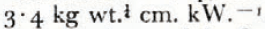 . The shape factor
Introduction
The performance of any type of thermal boring device, or “hotpoint”, that is drilling through clean, solid, temperate ice is entirely determined by the velocities, pressures, and temperatures in the warm melt water at the bottom of the hole. In the case of a hotpoint with a smooth, solid, impervious frontal surface nowhere heated above the local boiling temperature, herein termed a “solid-nose” hotpoint, this melt water flows outward in an extremely thin, and therefore non-turbulent, layer between the hotpoint and the ice. Because the flow is non-turbulent, it is possible to calculate the velocities, pressures, and temperatures from the equations of fluid mechanics, and thus to deduce theoretically the performance of the hotpoint.
In this paper the efficiency, the speed of penetration, and the temperature and distribution of pressure on the frontal surface are found as functions of the total input power, of the weight driving the hotpoint downward, of the shape and dimensions of the frontal surface, and of the pertinent physical properties of water and ice for the case of solid-nose hotpoints whose frontal surfaces are isothermal, axially symmetric, and either circular (non-coring) or annular (coring). The results are presented in graphical form in order to facilitate their practical use.
Theory
Coordinate systems. We define a set of circular cylindrical coordinates (r, z, ψ), fixed in the hotpoint, with the z-axis directed upward along the axis of symmetry. The radial coordinate r is then the perpendicular distance from the axis of the hotpoint. The angular coordinate ψ does not enter the problem because of the axial symmetry.
We also define a set of nearly orthogonal curvilinear coordinates (ξ, α, ψ), fixed in the hot-point, in which ξ is the arc length measured radially outward along the frontal surface, and α = ζ/h, where ζ is the distance measured perpendicularly away from the frontal surface and h is the local thickness of the layer of melt water. In the case of the circular hotpoint ξ is measured from the axis of symmetry; and in the case of the annular hotpoint it is measured from the inner edge of the frontal surface. The angular coordinate ψ is the same as in the cylindrical system.
These coordinate systems are shown in Figure 1.

Fig. 1. Coordinate systems
Symbols. The hotpoint has outside diameter 2a. It is assumed to be boring parallel to its axis vertically downward at a constant speed υ through clean, solid, temperate ice of density ρ i ( = 0·91 g. cm.−3). The heat of fusion of the ice is λ ( = 80 cal. g.−1). The melt water formed has density ρ w ( = 1·0 g. cm.−3), heat capacity c ( = 1·0 cal. g.−1 °C.−1), and thermal conductivity K ( = 1·4×10−3 cal. sec.−1 cm.−1 °C.−1). Only the viscosity μ. of the melt water varies significantly over the temperature range involved. It is given by the formula
where μ 0( = 1·8×10−2 dyne sec. cm.−2) is the viscosity of water at 0° C., and, η, which is plotted in Figure 2, is the specific viscosity of water. The thickness h of the layer of melt water is a function of ξ. The dependent variables u, υ, p, and θ are, respectively, the ξ-component of velocity, α-component of velocity, the pressure, and the temperature in the water layer.

Fig. 2. Specific viscosity of water as a function of temperature. The dimensionless temperature τ is defined by τ = θc/λ
Other symbols will be defined as they are needed.
Frontal surface. The profile of the frontal surface is described in the (r, z, ψ) coordinate system by the equation,
in which R must be a continuous, reasonably smooth function. The function R is subject to the further not very stringent restrictions that there be only one value of z for each value of R and that the radius of curvature of the frontal surface everywhere be large compared to the thickness of the water layer.
Fundamental equations. The variables u, υ, p, and θ must satisfy the continuity, momentum, and energy equations of fluid mechanics. We note that the Reynolds number will be small, that is, that

and that, in general,

As will be seen, restriction (3a) amounts to a restriction on the minimum permissible magnitude of dR/dz. We assume that the temperature θ is a function only of α, that viscous dissipation is unimportant, and that boiling does not occur. Because of these restrictions and assumptions many terms in the equations are comparatively negligible. Dropping these small terms, letting τ = θc/λ, and neglecting higher-order terms due to the very slight non-orthogonality of the coordinate system, we obtain the fundamental equations governing the velocities, pressures, and temperatures in the layer of melt water,


and

The derivation of equtions (4) is straightforward but lengthy. A good procedure is to write the fundamental equations in vector notation, then set the dilatation equal to zero (because the water is practically incompressible) and drop the acceleration terms (because the Reynolds number is small), and next by standard methods expand the remaining expressions in the (ξ, α, ψ) curvilinear coordinate system as if it were exactly orthogonal. The element of arc ds in the (ξ, α, ψ), system is given exactly by (ds)2 = g ξξ dξdξ + g ξα dξdα + g ξψ dξdψ + g αξ dαdξ + g αα dαdα + g αψ dαdξ + g ψξ dψdξ + g ψα dψdα + g ψψ dψdψ, in which the metric coefficients are given approximately by g ξξ = 1, g ξα = 0, g ξψ = 0, g αξ = 0, g αα = h 2, g αψ = 0, g ψξ = 0, g ψα = 0, g ψψ = R 2. The closeness of approximation, which mostly affects g ξξ , depends on how small the thickness of the water layer is in comparison to the radius of curvature of the frontal surface. Finally, by means of the remaining restrictions and assumptions many negligible terms maybe discarded, leaving only the dominant expressions in each equation.
Boundary conditions. The dependent variables must also satisfy certain boundary conditions, namely,


for both circular and annular hotpoints. In the case of the annular hotpoint, p is subject to an additional boundary condition,
where 2ϖ i a is the inside diameter of the hotpoint. For mathematical convenience both the atmospheric pressure and the hydrostatic pressure due to the water in the hole are dropped; the actual pressure can be found by adding them to p. The melting temperature of ice is arbitrarily taken to be zero in order to take advantage of the resulting simplification of condition (5c). The quantity dR/dξ is calculated from the relation,
Integration of the equations. Integrating (4b) twice with respect to α, using (4c) and the boundary conditions (5a), noting that the right-hand side of the second equation (5a) is negligible compared to the average value of u, and defining

we find

Substituting (8) into (4a), integrating once with respect to α, using the boundary conditions (5b), and defining

we obtain

Substituting (10) into (4d), we see that τ is a function only of α and hence the frontal surface of the hotpoint is isothermal, as previously assumed, provided

in which h 0 is an unknown constant length. Integrating (4d) twice with respect to α using (11) and the boundary conditions (5d), and defining

we find

in which β and γ are dummy variables of integration in place of α. The restriction (3a) on the Reynolds number is equivalent to B≪12
Equations (1), (7), (9), and (13) form a simultaneous system, valid for both circular and annular hotpoints, which can be solved numerically for the functions τ, η, and ϕ and the constant A corresponding to various values of B.
Performance of annular (coring) hotpoint. Continuity requires that

where Rm is the radius at which the pressure is greatest. Substituting (7) and (8) into (14), integrating by parts, using (7) and the boundary condition (5d), rearranging, and letting ϖ = R/a, we obtain

in which, from the boundary condition (5e),

where 2ϖ i a is the inside diameter of the hotpoint. The total weight driving the hotpoint downward is

in which the small contribution due to the viscous shear stress on the inclined portions of the frontal surface has been neglected. Substituting (15) in (16), integrating by parts, and letting

in which

we find

The “shape factor” S is a dimensionless number between 0 and 1 that depends only on the shape of the frontal surface, greater values of S being associated with blunter profiles; thus S = 1 for a plane frontal surface perpendicular to the axis.
The total input of power Q is equal to the rate at which heat is conducted away from the hotpoint, that is,

Eliminating h o and V, which are unknown, among (12), (17), and (18), we obtain

in which the dimensionless “performance number” N is given by

and the coefficient Λ is equal to
The efficiency E of the annular hotpoint is given by

it is defined as the ratio of the cross-sectional area of the hotpoint to the cross-sectional area of the hole it makes. The speed of penetration is, from (12) and (18),

The quantity (πρ i λ)−1 is equal to 37 m. hr.-1 kW.-1 cm.2. The temperature of the frontal surface is, from (13),

Finally, the distribution of pressure on the frontal surface is, from (15) and (17),

By means of equations (19) and (20) together with the numerical solution of (1), (7), (9), and (13) the desired parameters E, V, θ 0, and p describing the performance of the annular (coring) hotpoint can be calculated from the given quantities Q, W, and a, the given shape of the frontal surface, and the pertinent physical properties of water and ice.
Performance of circular (non-coring) holpoint. In the case of the circular hotpoint R m = 0, and the resulting equations are greatly simplified. The shape factor is given by

as in the case of the coring hotpoint, S is a number between 0 and 1, greater values of S being associated with blunter profiles. Some representative profiles and their shape factors are shown in Figure 3. The performance number for the circular hotpoint is given by


Fig. 3. Shape factors for some representative profiles of the frontal surface
in which the coefficient Λ as before is equal to

The speed of penetration is

in which the quantity (πρ i λ)−1 is equal to 37 m. hr.-1 kW.-1 cm.2. The temperature of the frontal surface is

Finally, the distribution of pressure on the frontal surface is

In complete analogy with the case of the annular hotpoint the performance of the circular hotpoint can be calculated from equations (21), (22), and (23) together with the numerical solution of (1), (7), (9), and (13) .
Numerical solution. Equation (1), (7), (9), and (13) are numerically solved for given B by a method of successive approximations. First, a trial temperature profile, τ as a function of α, is selected; next, the corresponding viscosity profile is determined (from, for example, Figure 2); then, ϕ is computed from (9) by numerical integration; and, finally, a new temperature profile is found in like manner from (13). This new temperature profile is then used as the starting point for the second cycle of the process, which converges rapidly, only a few cycles being needed to attain practical accuracy.
The approximation process is carried out for a number of values of B, and the corresponding values of E and τ 0 are obtained, from which the remaining parameters N and θ 0 are easily computed by means of (19), and (20) or (23). These quantities are tabulated in Table I for 12 values of B covering the range of practical interest. The quantity d is the maximum depth in water at sea-level at which boiling will occur at the corresponding temperature θ 0. Figure 4 shows the efficiency and the dimensionless surface temperature τ 0 plotted against the dimensionless performance number N; it summarizes in convenient form the main results of this paper.

Fig. 4. Efficiency, surface temperature and

Discussion
Drilling speed. The information presented in Table I and Figure 4 shows that the efficiency E of isothermal solid-nose hotpoints decreases with increasing performance number N. This raises the interesting possibility that the drilling speed V might actually decrease with increasing power input Q, inasmuch as the effect of the increased power input might be more than offset by the decreased efficiency. To show that this possibility does not arise in the range of N of practical interest, we differentiate (23b) with respect to Q, using (22) and the chain rule, then divide both sides by V and simplify, obtaining

Table 1. Summary of Numerical Results

An identical result will be obtained for the coring hotpoint by differentiating (20b) and using (19). The function −(dE/E)/(dN/N) is plotted against the performance number N in Figure 4. Because this function never exceeds unity in the range of N of practical interest, we conclude that the drilling speed always increases with increasing power input. The actual per cent increase in V per per cent increase in Qvaries from 1.00 for N = 0·0 to 0.59 for N = 4·0.
Similar calculations show that for both circular and annular hotpoints


and

The per cent increase in V per per cent decrease in a varies from 2.00 for N = 0.0 to 1.59 for N = 4.0. Over the same range the per cent increase in V varies from 0.00 to 0.10 to per per cent increase in W, and from 0.00 to 0.41 per per cent decrease in S or N. Thus, over the whole range in N for which the theory is valid, the drilling speed of isothermal hotpoints varies in a simple manner with respect to variations in design or operation.
Effect of turbulence. Though the theory presented in this paper is quantitatively valid only for non-turbulent flow in the layer of melt water between the hotpoint and the ice, it can give a semiquantitative indication of the effect of turbulence in the layer of melt water on the performance of an isothermal hotpoint. For fully developed turbulence Ke ≈ 2cμe , where K e is the eddy conductivity and μ e is the eddy viscosity, which will be of order 102 times the molecular viscosity μ 0. Substituting these values into the expression for Λ in (19a), we find that Λe ≈ Λ/30, hence N e ≈ N/30, and therefore that, other things being equal, turbulence in the layer of melt water should remarkably improve efficiency. Partially developed turbulence should have a similar but smaller effect.
Isothermal restriction. The assumption that the frontal surface is isothermal corresponds to the assumption that it is composed of material with infinite thermal conductivity, or has a special shape. For real materials and nearly all shapes the boundary condition at the frontal surface will in general be a functional relationship between the temperature τ and its normal derivative ∂τ/∂ζ on the surface ζ = 0; this relationship can in principle he found by solving the heat-flow equation for the interior of the hotpoint (assuming that the magnitude and distribution of all heat sources and sinks except the frontal surface are known). Only in specialcases will the relationship required by the theory presented in this paper be satisfied, namely,

where τ o is a constant temperature and q o is a constant heat flux independent of position. Note that implicit in the condition that the frontal surface be isothermal is the further condition that the flow of heat through any element of area of the frontal surface be proportional to the area of the projection of the element on a plane perpendicular to the axis of the hotpoint.
One way to test the assumption for a given design is to calculate, by numerical methods, if necessary, the heat flow at the frontal surface that would occur if the surface were actually isothermal. The degree to which this calculated heat flow agrees with the required heat flow is a measure of the applicability of the theory. A misfit of a few per cent probably is not crucial. In any case, if the calculated value of q o increases with increasing ξ, then the hotpoint will be less efficient than predicted by the theory, and conversely. This follows because, if q o is less at the center, the “cool” center will be “slower” than the hotter outer zone of the frontal surface, hence the effluent melt water at the outer edge of the hotpoint, being hotter, will carry away a larger fraction of the total heat available.
Effect of corrosion. If the frontal surface of an isothermal hotpoint becomes coated with a thin layer of poorly conducting material, for example by becoming corroded, the drop in temperature across the insulating layer will be greatest where the heat flow is greatest. Thus, by the same reasoning as for the non-isothermal hotpoint, if dR/dξ decreases with increasing ξ (the usual case), then corrosion will cause a decrease in efficiency, and conversely.
Design of hotpoints. Although the theory presented in this paper applies specifically to isothermal hotpoints, it can also be used to estimate the approximate drilling speed and efficiency of non-isothermal designs in terms of power input, driving weight, inside and outside diameter of hotpoint, and shape of frontal surface, thus facilitating selection of the optimum design for a given application without the time and expense of building and testing a long series of prototypes. Even more important, it enables the designer to estimate at least approximately two other highly important parameters in the design, the temperature of the frontal surface, and the magnitude and distribution of pressure on it, thus permitting much smaller factors of safety than would otherwise be possible.
Acknowledgements
This problem was formulated and partially solved while I was a National Science Foundation postdoctoral research fellow at the Swiss Federal Institute of Technology. Professor Dr. G. Schnitter, Director of the Laboratory for Hydraulic Research and Soil Mechanics at the Institute, and Ing. P. Kasser, Chief of the Section for Hydrology and Glaciology of the Laboratory, generously gave me free use of space and facilities, and otherwise indirectly contributed to the work reported in this paper.Footnote * I am pleased to express here my appreciation to Dr. W. H. Ward and Professor W. B. Kamb for reading and commenting on the original manuscript; their suggestions have resulted in a number of significant improvements in this paper, though, of course, they do not thereby undertake responsibility for any of its contents. I also wish to thank Professor Gerhard Oertel for helping me with the German abstract. The numerical computations were performed on the Bendix G-15 computer in the Institute of Geophysics of the University of California.


