Effect of Sea-Ice Structure

Structurally undeformed first-year sea ice is very similar to a cast ingot. Its uppermost zone (the initial skim) is produced by the formation of the initial ice layer across the sea surface. This layer may vary from a few millimeters to 20 cm in thickness depending on the sea state at the time the ice cover forms. The layer below this can be referred to as the transition zone, in that a preferred growth orientation develops in the crystals. Although these upper two layers are quite interesting from a crystal-growth point of view, they are usually very thin (the base of the transition zone is commonly less than 30 cm below the upper surface of the ice sheet), and do not need to be considered for most engineering purposes.

During the melt season, the upper two layers commonly ablate away causing multi-year ice to be essentially completely composed of ice of the third zone. The ice of this so-called columnar zone characteristically has a strong preferred growth fabric with the crystals elongated vertically parallel to the direction of heat flow and the c-axes of the crystals oriented almost perfectly in the horizontal plane. This results in the basal planes of the ice crystals being oriented in a near-vertical direction. The geometric selection that occurs, as crystals with their c-axis oriented close to horizontal cut out other less fortunately oriented crystals, causes a gradual increase in grain size with depth at least in the upper portion of the ice sheet. In fact the very limited number of measurements of grain size (Reference WeeksWeeks and Assur, 1967) suggests that the mean crystal diameter increases with depth at a rate independent of the grain size present at the base of the transition zone. Because the size of the crystals becomes large relative to that of the samples usually taken, adequate descriptions of grain-size variations are only available for the top 60 cm of first-year ice. Limited observations of the lower portions of 2 m thick ice show large areas (at least 1 m in diameter) that have roughly collinear c-axis orientations (Reference PeytonPeyton, 1966). Although the degree of colinearity is not sufficient for such areas to be considered as single crystals (unpublished results of A. J. Gow and W. F. Weeks), the degree of preferred orientation would clearly result in large variations in physical characteristics such as ice strength with changes in the direction of loading. In fact in the old sea ice, that was incorporated in the ice island ARLIS II, Reference SmithSmith (1964) reported areas of collinear c-axis that are as large as 10 m on a side, and recent studies of the anisotropy of the electrical characteristics of first-year ice have suggested that these domains may be very large (Reference Campbell and OrangeCampbell and Orange, 1974).

Each individual crystal of sea ice is sub-divided into a number of ice platelets that are joined together to make a sort of a quasi-hexagonal network as viewed in the horizontal plane. It is within this network that most of the entrapped brine present in the sea ice is believed to be located. Figure 1 presents a schematic view of a cross-section of first-year sea ice. Also shown are several sketches made from thin sections showing both the individual crystals and the ice platelets, and a close-up of the brine pockets located between the platelets. The width of the platelets a_o, the so-called plate spacing, varies systematically with the ice growth velocity. Observations in metals suggest a fundamental relationship of the general form,

where v is the growth velocity and c is a constant. Limited observations on a_o variations in NaCl ice (Reference Lofgren and WeeksLofgren and Weeks, 1969) suggest that the power of v may actually be a function of v. In any case, the slower the ice grows, the wider the ice platelets, resulting, in most situations, in a_o increasing with increasing depth in the ice sheet. Other aspects of the geometry of these platelets or of the details of the geometry of the brine layers, channels and pockets have only received cursory examination. It is, however, reasonable to expect that they will also prove to be a function of the ice growth velocity.

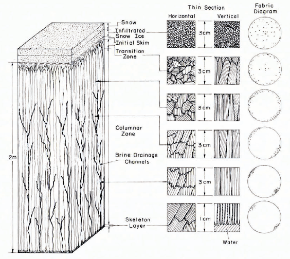
Fig. 1. Schematic drawing showing several different aspects of the structure of first-year sea ice.

One other aspect of the sea-ice substructure should be mentioned here. As the brine initially trapped between the ice platelets drains down and out of the ice sheet, it moves through structural features within the ice that have been referred to as brine drainage channels. These channels can be thought of as tubular river systems in which the tributaries are arranged with cylindrical symmetry around the main drainage channels. In first-year ice, such channels do not appear to reach above the base of the transition zone, presumably indicating that a certain volume of ice is required as a source of brine before a channel can form (or be identified). Near the bottom of thick annual sea ice, drainage channels appear to occur on a horizontal spacing of 15 to 20 cm and have a diameter of approximately 1 cm. The presence of drainage channels is also schematically illustrated in Figure 1.

Although all aspects of the structure of sea ice should influence its physical properties, at the present only the substructure associated with the presence of the ice platelets has been considered; all the salt is taken as entrapped in channels, layers, and pockets (or at very low temperatures as crystals of solid salt) between these plates. A drawing showing this idealization as developed by Reference AssurAssur (1958) is given as Figure 2. It is also assumed that the failure planes within each ice crystal will largely coincide with the planes along which the salt is concentrated. This assumption is borne out by a limited number of observations of the geometry of actual failure surfaces in natural sea ice (Reference Anderson and WeeksAnderson and Weeks, 1958; Reference TabataTabata, 1960). The reason for this coincidence is that the salt inclusions reduce the effective cross-sectional area of ice-to-ice bonding between the plates causing the interplate boundaries to be planes of weakness. Therefore it is reasonable to suppose that variations in the failure strength σ_f of sea ice can be expressed in the general form

where ψ is the plane porosity (the relative reduction in the area of the failure surface caused by the presence of gaseous and liquid inclusions) and σ_o is the so-called basic strength of sea ice (the strength of an imaginary material containing no brine or air but still possessing the sea-ice substructure). The critical value of ψ along the failure plane is

where v, v_a, and v_b are respectively the volume of void, or the porosity, of air and of brine. It then only remains to express ψ in terms of v via a model for the geometry of the inclusions. This has been done by Reference AssurAssur (1958), Reference Anderson and WeeksAnderson and Weeks (1958), and (Reference AndersanAnderson 1958[a], Reference Anderson1960). Details on these treatments can be found in (Reference WeeksWeeks and Assur 1967, Reference Weeks and Assur1969) and need not concern us here. The results of the analysis give an equation of the general form

where c and k are constants the values of which depend upon how the geometry of the fluid inclusions varies with changes in v. Models that have been considered include ones in which the brine pockets remain a constant width (k = 1) or show geometric similarity on a horizontal plane (k=½) or in space (k=2/3). In fact the detailed petrographie observations necessary to indicate which model most closely approximates reality are lacking. However, most recent authors have satisfactorily used k = ½ to correlate changes in σ_f with changes in v and we will also present available data in this form. On such plots the value of σ₀ is given by the intercept of the linear extension of the least-squares straight line through the data with the σ_f axis.

Fig. 2. Idealized diagram showing the shape of the brine inclusions in sea ice and parameters used to describe them (Reference AssurAssur, 1958).

As will be discussed later, similar variations in many other physical properties of sea ice are also caused by changes in v. It is upon this dependence that the estimation of the engineering properties of sea ice is usually based. Design values are usually extreme values which are difficult to measure in the field because they occur so rarely. However, if the value of v associated with the extremes can be estimated, then one can simply determine the value of the physical property of interest from its measured or extrapolated dependence upon v. In fact, this is not too difficult to do because the salinity of sea ice changes rather systematically with ice thickness and age. Attempts to present these types of correlations for both average salinities and salinity profiles can be found in (Reference WeeksWeeks and Assur 1967, Reference Weeks and Assur1969), Reference Cox and WeeksCox and Weeks (1974), and Reference TsurikovTsurikov (1976). This compositional information can then be combined with representative ice temperatures, which can be estimated from information in Reference PeschanskiyPeschanskiy (1967), Reference Maykut and UntersteinerMaykut and Untersteiner (1969), and Reference MaykutMaykut (1976).

For instance, if we are interested in the tensile strength and elastic modulus profiles for 0.2, 0.8 and 3.0 m thick ice in the Arctic Basin on roughly 1 May, we would expect values similar to the profiles shown in Figure 3. Here we have converted the estimated salinity and ice temperature profiles to a brine volume profile via the empirical relation developed by Reference Frankenstein and GarnerFrankenstein and Garner (1967) from the brine volume tables for standard sea ice worked out by Reference AssurAssur (1958). In doing this, we have not taken account of the volume of gas entrapped within the ice. Although for first-year ice this volume is usually believed to be small relative to the brine volume, this may not be true for multi-year ice. In converting from brine volume profiles to σ_f/σ_oand E/E_o profiles, the equations suggested by Reference DykinsDykins (1971) and by Reference Langleben, Pounder and KingeryLangleben and Pounder (1963) for flexural strength and dynamically determined elastic modulus were used. As will be discussed later, the problems in preparing such profiles are primarily caused by uncertainties in the values of the engineering parameters of interest near the melting point (large v) and at temperatures colder than — 23˚C (presence of significant amounts of solid salt in the ice). Once adequate physical property profiles have been obtained either by the methods that we have described or by direct measurement, methods for deducing proper composite characteristics for the ice can be applied (Reference Assur and Ōura.Assur, 1967; Reference WeeksWeeks and Assur, 1967).

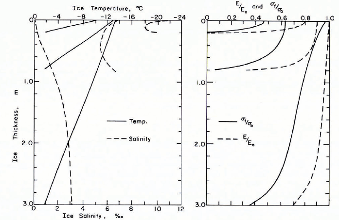
Fig. 3. Representative sea-ice temperature, salinity, EǀE₀ and σ_fǀσ₀ profiles for 0.2, 0.8, and 3.0 m thick Arctic sea ice on c. 1 May. To convert σ_fǀσ₀ to σ_f and EǀE₀ to E multiply by 10.3 X 10⁵ Nǀm² and by 10¹⁰ NǀM² respectively based on the flexural strength determinations by Reference DykinsDykins (1971) and the elastic modulus measurements by Reference Langleben, Pounder and KingeryLangleben and Pounder (1963).

Engineering Properties of Sea Ice

There are, of course, a large number of material characteristics of sea ice that can legitimately be considered of engineering interest. Fortunately, in most problems one needs to be concerned with only a small number of these. We can discern what these properties are by listing first some of the more important applied areas of concern, then a few more specific problems in each of these areas, and finally the engineering properties of sea ice required to resolve these problems. This is done in Table I. Although this table does not attempt to provide an inclusive list of problems, it is clear that certain engineering properties of sea ice would occur over and over in any such list that is prepared. These are the mechanical properties as they relate to both short-term and long-term loading and to ultimate failure of the ice, the fractional properties which must be considered when ice bonds to or moves relative to either an engineering structure or to itself, and the thermal properties which are essential to any problem in which ice growth or the change in temperature of the ice is important. Finally, there are the electromagnetic properties of the ice which must be understood to obtain maximum benefit from the application of current remote-sensing technology to sea ice. It is these techniques that will provide the requisite descriptions of areas of pack ice that should be available before sound engineering calculations can start.

TABLE I. DATA REQUIREMENTS FOR SELECTED PROBLEMS IN SEA-ICE ENGINEERING

Mechanical Properties

Although sea ice is the main engineering concern in the development of Arctic navigation and off-shore technology its mechanical properties have been investigated far less than those of fresh-water ice. In fact, in the last four symposia dealing with the engineering aspects of ice in which 250 papers were presented, only 10 dealt with the mechanical properties of sea ice. One reason for this situation is that properties such as failure strength, elasticity, plasticity, stress-strain behavior, and the fracture modes under various load conditions arc presumably complicated by the presence of brine inclusions, which do not occur in relatively pure freshwater ice. Also frozen lakes are readily accessible from many locations while studies of sea ice invariably involve considerable logistic effort and expense.

Even though some work has been done on each of the mechanical properties, the evaluation and comparison of results is, at best, difficult, since the methods of testing commonly differ from one investigator to another. This lack of standardization has proven to be such a problem that the Committee on Ice Problems of the International Association for Hydraulic Research (IAHR) has formed a Standardization Task Group to make recommendations in this regard. We will refer to their first report (Reference FrankensteinIAHR, 1975) several times in the following discussion.

Strength

Compressive strength

(a) Testing procedures

In the conventional uniaxial compression test, axial force is applied to the ends of a specimen through steel platens that make direct contact with the test specimen. Friction between platen and specimen produces radial restraint, so that there is commonly a triaxial state of stress near the end planes. The triaxial field is significant over an axial distance from the end planes of about one specimen radius. Interposition of highly compliant sheets (elastic or plastic) between the platens and the specimen often changes the sign of radial end forces, but does not eliminate the triaxial stress state. On a different scale, irregularities in the specimen end planes also create localized stress perturbations, and in brittle material these commonly initiate microcracks that lead to premature failure of the specimen.

Most attempts to overcome all these difficulties have been unsuccessful. Therefore the usual procedure has been to use a specimen that is long enough to provide a mid-section that is reasonably free from end-effect stress perturbations.

The International Association for Hydraulic Research (IAHR) Standardization Task Group has suggested a new method for testing ice in compression by using low-modulus urethane which is laterally confined by an aluminum cylinder to prevent radial deformation. This method has been tested and found to be satisfactory in the sense of providing reasonable approximation to a uniaxial state of stress throughout the specimen. It also allows for reasonable tolerances in specimen preparation and permits the use of smaller specimens. For more information see either the Task Group report (Reference FrankensteinIAHR, 1975) or Reference Haynes and MellorHaynes and Mellor (1977). However, as of the present, this method has not been utilized in studies of sea ice.

(b) Load direction

The earliest simple compression tests on cylinders of sea ice were carried out by (Reference ButkovichButkovich 1956, Reference Butkovich1959) who obtained strength values ranging from 76 × 10⁵ N/m² at —5°C to roughly 120 × 10⁵ N/m² at — 16°C from vertical cores. Average values on horizontal cores in the same temperature range varied from 21 × 10⁵ to 42 × 10⁵ N/m². A similar strong orientation dependence was found by Peyton (1966) who ran tests on a large number of samples of different sea-ice petrographic types at various orientation and stress rates (Fig. 4). The ice Peyton used characteristically had grain sizes larger than the diameter of his specimen. Therefore, his samples were essentially single crystals with their c-axes oriented parallel to the plane of the ice sheet. In Figure 4 the loading-angle notation is as follows: the first number gives (he angle between the axis of the test cylinder and the vertical, while the second number gives the angle between the sample and the c-axis of the single ice crystal being tested. Note that the ratio of the strength obtained from vertical cores to that obtained from horizontal cores is about 3 to 1 which is in agreement with the results of Reference ButkovichButkovich (1959).

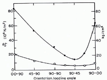
Fig. 4. Average failure strength in compression (solid circles) and in direct tension (open circles) versus sample orientation: bottom ice, —10°C (Reference PeytonPeyton, 1966). For orientation notation see text.

In contrast to these findings are results of compressive strength tests carried out by Reference SchwarzSchwarz ([1971]) on saline ice from the western part of the Baltic Sea. The salinity of this ice was 2.7%₀ due to the high rate of freezing (12 cm in 36 h). As shown in Figure 5, the strength was about 20% higher when the ice was compressed in the horizontal rather than in the vertical direction. Because similar results in respect to the effect of the direction of load on the compressive strength have reportedly been obtained in proprietary studies sponsored by oil companies, the whole matter needs to be reconsidered. In further studies the failure mode and the strain conditions in the three principal directions of deformation as well as the structure of the ice should be investigated in order to remove some of the ambiguity in explaining the results.

Fig. 5. Compressive strength of Baltic Sea ice as a function of strain-rate, ice temperature, and orientation of the force (Reference SchwarzSchwarz, [1971])

It has been argued in explaining Peyton’s and Butkovich’s results that the grain boundaries and the basal planes of individual crystals, which are the planes where the brine pockets are located, are oriented so the specimen will fail easier when loaded perpendicular to the direction of growth. Other arguments can be formulated to explain Schwarz’s results: sea ice fails most easily in tension by separation of the ice crystals along their long axis. This is what has been observed to happen in the uniaxial state of stress when a sample is loaded parallel to the direction of growth (which is also the direction of the long axes of the crystals) and subsequently fails by tensile strain perpendicular to the direction of load (Reference WuWu and others, 1976).

(c) Brine volume

Peyton’s results on the variation of the compressive strength of sea ice with changes in the brine volume are shown in Figure 6. Here σ_R is a strength index (the measured compressive strength corrected for variations in the rate of application of the stress; where σ_c is the compressive strength, is the rate of stress application and b is an experimental constant equal to 0.22). Different interpretations can be placed on this data as indicated by the solid and dashed lines. The solid line suggested by Reference WeeksWeeks and Assur (1967) is

where σ_R was defined as mentioned and v_b is the absolute value of the brine volume. This relation holds only at v_b ⩽ 0.25. At higher values of v_b, σ_R is assumed to be constant independent of v_b in agreement with similar observations in in-situ cantilever beam tests, shear tests and ring-tensile tests. The dashed line, suggested by Reference PeytonPeyton (1966), will be discussed later. The significant feature in these results is that both sets of investigators felt that σ_R could be adequately expressed as a function of the square root of the brine volume.

Fig. 6. σ_R from compression tests versus square root of the brine volume (Reference PeytonPeyton, 1966). For the difference between the solid and dashed lines see discussion in text.

(d) Temperature

The effect of temperature on the compressive strength has only been considered in connection with the brine volume. Peyton found the ice strength obtained at temperatures below —8.7°C to be significantly greater than extrapolated values based only on tests from warmer ice (see the dashed line in Figure 6). This was explained by the fact that at — 8.7°C Na₂SO₄· ₁₀H₂O starts to precipitate. This solid salt was suggested to strengthen the ice in a manner similar to steel in concrete. Tests of Reference SchwarzSchwarz ([1971]) lend some support to this explanation since his investigation on saline ice from the Baltic Sea shows a relatively steeper increase of the strength between —10 and — 20°C compared with equivalent tests on freshwater ice (Fig. 7). The results are hardly conclusive.

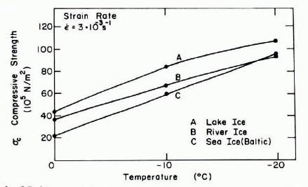
Fig. 7. Compressive strength of Baltic ice and freshwater ice as a function of temperature (Reference SchwarzSchwarz, [1971]). Load applied perpendicular to the growth direction.

(e) Strain-rate

From compressive strength tests on fresh-water ice we know that ice has a failure strength maximum at a certain strain-rate. In this respect Peyton found contradictory results for sea ice from different locations. For sea ice from Point Barrow the strength increased with the stress rate while for sea ice from Cook Inlet the strength decreased when tested at the same loading rates.

In spite of these non-conclusive results Peyton expected the failure strength to have a maximum at a certain stress rate. This assumption was confirmed by Reference SchwarzSchwarz ([1971]) who investigated the strength of saline ice from the Baltic Sea at different strain-rates and temperatures. The results given in Figure 5 clearly indicate a maximum failure strength at a strain rate of about 10^–3 s^–1 which is associated with the transition between creep-ductile and brittle failure. The same phenomenon has been found in compression tests of fresh-water ice (Reference CarterCarter, [1972]; Reference KorzhavinKorzhavin, 1962; Reference WuWu and others, 1976; Reference SchwarzSchwarz [1971]). There is still discussion as to whether or not the compressive strength decreases at higher strain-rates. Reference CarterCarter ([1972]) explains the decrease of strength at higher strain-rates by energy considerations. He shows that the stress concentrations occurring at the tip of cracks are reduced by plastic deformation. Therefore at high strain-rates there is less time for plastic deformation and as a result the strength decreases. Reference Hawkes and MellorHawkes and Mellor (1972) believe the decrease is a result of poor experimental methods. With the new testing method suggested by the I.A.H.R. Standardization Task Group and also with the improvements in available testing machines it should be possible to establish reliable results on such relationships. Furthermore, ice temperature should not be overlooked as an important parameter in connection with the strain-rate. This has, as yet, not been investigated for sea ice, but from testing fresh-water ice (Reference CarterCarter, [1972]; Reference WuWu and others, 1976) we know that the relation between strength and strain-rate is temperature dependent. Due to the correlation between temperature and the brine volume of the ice, the strain-rate effect will also be a function of the brine volume.

(f) Size effect

Investigations on fresh-water ice have shown that the compressive strength increases if the ratio of crystal size to sample size exceeds a certain value. This so called “size effect" has not, as yet, been investigated for sea ice. Due to the substructure of the crystals and the possibility of easy crack propagation across the crystals on planes of impurities it is very likely that the size effect will not occur in sea ice. This, of course, needs to be proven.

(g) Conclusions

The controversial results and the gaps of knowledge on the uniaxial compressive strength of sea ice should be a challenge for further intensive studies on this subject. In order to be able to make both qualitative and quantitative comparisons of the results of different investigators it is suggested that the recommendations for testing ice in compression of the I.A.H.R. Standardization Task Group be carefully considered in designing any such studies.

Tensile strength

Uniaxial tensile strength can only be determined unambiguously through direct tension tests. Any substitute for direct testing methods such as ring-tensile, brazil, or beam tests induces complicated stress states within the sample which require assumptions about the stress-strain relationship before strength values can be calculated from the test results.

The most comprehensive work on the tensile strength of sea ice has been carried out by Reference DykinsDykins (1970) and has also been summarized by Reference Katona and VaudreyKatona and Vaudrey (1973). The ice investigated was frozen from sea-water in a laboratory tank to simulating freezing conditions in nature. The salinity within the ice was 1 to 2‰ (brackish ice) and 8 to 9‰ (sea ice). By varying the temperature, a wide range of brine volumes was investigated. The tests were carried out on dumb-bell specimens which were attached to the testing machine by gripping heads. A similar method in which the ice was frozen to metal end cups has been used by Reference Hawkes and MellorHawkes and Mellor (1972). Both methods provide a fairly accurate uniaxial state of stress as photoelastic observations by G. D. Vaudrey (personal communication) have shown. With minor improvements by Reference Hawkes and MellorHawkes and Mellor (1972) this method has been suggested for tension tests by the Standardization Task Group.

Reference DykinsDykins (1970) results have shown a very strong difference in the tensile strength depending on the direction of load: the ice was two to three times stronger when the tension was applied in the vertical direction than in the horizontal (Fig. 8). This result supports the compression test results on sea ice of Schwarz (Fig. 5), since compression applied in the vertical direction induces tensile strain in the lateral direction.

Fig. 8. Tensile strength of sea ice versus the square root of the brine volume (Reference DykinsDykins, 1970).

Figure 8 shows that the tensile strength, in the vertical as well as horizontal loading direction, can be adequately expressed as a function of the square root of the volume, similar to the case for compressive strength. The equations derived from the two curves of Figure 8 are:

Dykins stated that the tensile strength was not appreciably dependent on the crystal size. Since the ratio of dumb-bell diameter to crystal diameter was as low as five, the so-called size effect should have shown up if it is present in sea ice. These results indicate that the substructure of a sea-ice crystal works like the grain boundaries in fresh-water ice in respect to easy crack propagation.

Limited studies on the effect of stress rates on the tensile strength show strength to be insensitive to stress rates ranging from to . A similar result was found by Reference Hawkes and MellorHawkes and Mellor (1972) in tensile tests on fine-grained fresh-water ice. However, for stress rates greater than 1.8 × 10⁵ N/m² s, Reference DykinsDykins (1970) observed that the tensile strength decreased by 52% of the initial value. This result can be explained by the higher number of stress concentrators within sea ice in the form of brine pockets and air bubbles which become more effective at higher stress- or strain-rates.

Even though the tensile-strength tests of Dykins were carried out well, more testing of the tensile strength is necessary to confirm his results and to answer remaining questions such as the strain effect in relation to the brine volume, the precipitation of solid salts and their influence on the tensile strength, and the failure mode at various strain-rates. Further testing should also be expanded to include tensile-strength behavior under three-dimensional stress states.

Flexural strength

The flexural strength is not a basic material property but only an index strength. It is normally obtained by two different test methods: simply-supported beam tests or cantilever beam tests. The cantilever beam tests have an advantage in that they can be easily carried out in the field, thereby avoiding major brine drainage.

As Reference GowGow (1977) has shown in a paper presented earlier at this conference, cantilever beam tests on fresh-water ice provide a flexural strength which is up to 50% less than the flexural strength obtained from simply supported beams. Gow suggests that this difference is the result of stress concentrations occurring at the butt end of the beams. In sea ice such significant differences in strength have not been reported; on the contrary, it has been stated (Reference FrankensteinFrankenstein, 1968) that the results obtained by these two testing methods vary only slightly. This characteristic of sea ice is probably due to its more plastic behavior which relieves the stress concentrations and results in higher strengths.

The flexural strength of cantilever beams has usually been calculated as

where P is the failure load, l the length, b the width, and h the thickness of the beam.

This equation assumes that the deformation is elastic and the material is both isotropic and homogeneous. Sea ice, however, is an anisotropic material with a non-linear stress distribution over the beam depth. Reference HutterHutter (1973) has developed an equation which considers these conditions; its application, however, is difficult, because it requires the establishment of a stress distribution according to the temperature and salinity gradient. Therefore, for practical uses and for the purpose of obtaining some index strength the equation given above may be sufficient.

On the other hand we should not forget that certain controversial results have been reported, for example by Reference LavrovLavrov (1969), using the equation based on the elastic theory for beams of different dimensions. It is very likely that these and other peculiar results of ice tests are due to the incorrect assumptions with regards to the material properties. If, for practical reasons we continue to use equations based on the elastic theory for calculating the flexural strength, then more testing is necessary to elucidate the size effect and to standardize the testing methods, i.e. beam preparation, loading conditions, etc.

Many investigators have determined values for the flexural strength of sea ice. The relation between brine content and flexural strength as determined from in-situ cantilever beam tests is particularly consistent, as shown in the investigations of Reference Weeks and AndersonWeeks and Anderson (1958), Reference Brown and KingeryBrown (1963), and Reference ButkovichButkovich (1956) (Fig. 9). From Figure 9, the equation obtained for σ_f as a function of v_b is

for v_b^½ < 0.33. These results suggest that the flexural strength remains roughly constant for brine volumes for which v_b^½ > 0.33. However, this constancy of strength was not obtained by Reference Schwarz and FrankensteinSchwarz (1975) in his investigation of high salinity ice produced for model studies.

Fig. 9. Flexural strength measured by in-situ cantilever beam tests versus square root of the brine volume.

The most recent and extensive work on the flexural strength was done by Reference DykinsDykins (1971) who tested large in-situ beams with ice thicknesses of up to 2.4 m. His test results (see Fig. 10) are well described by the equation

Fig. 10. Flexural strength as measured by fixed-end and simply supported beams versus brine volume (Reference DykinsDykins, 1971).

A comparison of the results of Figures 9 and 10 shows that in both cases the curves have similar slopes as well as similar intercepts on the flexural-strength axis. This strongly suggests that external stress concentrations at the sharp corner of the butt of the cantilever are quite small. This had been already postulated by Reference FrankensteinFrankenstein (1968).

Strength tests with different stress- or strain-rates have shown quite contradictory results. Reference Tabata and ŌuraTabata and others (1967) have tested cantilever beams of sea ice—even recently in the Gulf of Bothnia (Reference TabataTabata and others, 1975)—at stress rates up to about 3 × 10⁵ N/m² s. They found a considerable increase of the flexural strength of sea ice with increasing stress rates. However, if the inertial force associated with the displacement of the water during rapidly performed tests is eliminated (Reference MäättänenMäätänen, 1976), the flexural strength of sea ice appears 10 be almost independent of the stress rate.

Even though the flexural strength is not a basic material property, it is relatively easy to obtain, and therefore it is commonly used as an indicator of the strength of ice. Our present knowledge of the flexural behavior of sea ice, however, is not sufficient for us to obtain reproducible and consistent results. Questions such as the size effect, the failure mechanism, and the shear involvement in the failure of beams, remain unresolved.

Shear strength

Only a small number of shear-strength tests have been carried out and reported. In fact, many tests described as “shear" are actually the result of mixed-mode failures as in punch tests. Indeed, it is extremely difficult to obtain pure shear strengths. The best sets of shear-test data available are those of Reference Paige and LeePaige and Lee (1967) and of Reference DykinsDykins (1971). Reference Paige and LeePaige and Lee’s (1967) results show similar trends with brine volume changes (Fig. 11) as do in-situ cantilever beam tests (Fig. 9). Also the absolute value of the shear strength is in the range of observed flexural and tensile strengths (with tension applied parallel to the growth direction). Reference DykinsDykins (1971) found the shear strength of sea ice to be not appreciably affected by different crystal orientations. This indicates again that not only arc grain boundaries and the basal planes of ice crystals lines of easy slip but that the same is also true of planes within the substructure where brine pockets and imperfections are lined up.

Fig. 11. Shear strength as a function of the square root of brine volume (Reference Paige and LeePaige and Lee, 1967).

Even though the few results available indicate a strong dependency of the shear strength on the load or strain-rate, this effect cannot yet be quantified. This is an area requiring more thorough investigations.

Some contradictory results on the effect of temperature on shear strength have been reported by Reference Katona and VaudreyKantona and Vaudrey (1973). On the one hand, shear strength increased significantly in a similar fashion to other strength results when the temperature was lowered from –2 to —10°C. On the other hand, the shear strength was lower at —10°C than at —4°C and greater at —20°C than at —27°C. This last result is probably incorrect, but it is mentioned here in order to show the gaps and to stimulate further investigations, especially on shear strength, which has been widely disregarded in the past.

Elastic Modulus

There has not, as yet, been an adequate theoretical treatment of the variation in the elastic modulus of sea ice with brine volume and crystal orientation based on a realistic model of the arrangement of inclusions in sea ice. Even so, current experimental observations are in general agreement with theoretical predictions for materials with a random distribution of pores in that the variation in E with the volume fraction of pores is to a good approximation linear in the porosity range 0 to 10% (Reference Coble and KingeryCoble and Kingery, 1956; Reference Buch and GoldschmidtBuch and Goldschmidt, 1970), which is the range in which sea ice has primarily been studied.

Dynamic measurements

By dynamic measurements of the elastic modulus E we mean values determined by cither the rate of propagation of vibrations in the ice or by exciting natural (resonant) frequencies of different types of vibrations. The displacements in such measurements are extremely small and, for many purposes, anelastic effects can be neglected. Therefore, dynamic measurements ot E tend to be quite reproducible when compared with E values determined from typical mechanical tests.

In-situ seismic determinations of E for natural sea ice have been reviewed by Reference WeeksWeeks and Assur (1967), More recent results have been reported by Reference KohnenKohnen (1972). E was found to vary from (1.7 to 5.7) × 10⁹ N/m² when measured by flexural waves and (1.7 to 9.1) × 10 N/m² when determined by in-silu body-wave velocities. The E values when measured on similar ice, are invariably larger when determined by body waves. This is reasonable inasmuch as the flexural-wave velocity is controlled by the overall properties of the ice sheet while the body-wave velocity is controlled by the high-velocity channel in the usually colder and stiffer upper portion of the ice. Pronounced changes in E are noted throughout the year with high values occurring in winter (cold, low brine volumes) and low values in the summer (warm, high brine volumes). Detailed studies of the relation between E and brine volume have been made by Reference Anderson.Anderson (1958[b]) and Reference Brown and HowickBrown and Howick (1958). Both test series show a pure-ice intercept at zero brine volume of (9 to 10) × 10⁹ N/m² and a pronounced decrease in E as v_b increases. The Anderson’s results are shown in Figure 12.

Fig. 12. Elastic modulus of sea ice as determined by seismic techniques versus brine volume (Reference Anderson.Anderson, 1958[b]). The three triangular points are the results of static tests performed by Reference DykinsDykins (1971).

The remainder of the dynamic determinations of E were made on small specimens which had been removed from the ice sheet. A representative series of tests performed by Reference Langleben, Pounder and KingeryLangleben and Pounder (1963) is shown in Figure 13. E values at zero brine volume are characteristically found to be (9 to 10) × 10⁹ N/m², in good agreement with the seismic determinations. The decrease in E with increasing v_b appears to be linear within the range of brine volumes studied. Recent studies suggest that at v_b values greater than 0. 1 the value of E decreases more slowly becoming a weak function of v_b at v_b values in excess of 0.15 (Reference Slesarenko and FrolovSlesarenko and Frolov, [1974]). This is in general agreement with theoretical predictions (Reference Coble and KingeryCoble and Kingery, 1956; Reference Hashin and WendtHashin, 1970). However in these predictions, appreciable deviations from a linear relation do not occur until porosity values become larger than 0.2.

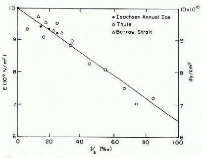
Fig. 13. Elastic modulus of cold arctic sea ice as determined by small specimen lests versus brine volume (Reference Langleben, Pounder and KingeryLangleben and Pounder 1963)·

Static measurements

Static measurements of E are much more variable and difficult to interpret than are dynamic measurements because of the visco-elastic behavior of ice when subjected to significant stresses for finite time periods. Nevertheless static measurements are extremely important as they are required in the consideration of problems such as ice forces on structures and vessels and bearing-capacity calculations.

The most extensive study of the static modulus of sea ice is by Reference DykinsDykins (1971) who tested small beams in bending. His stress-strain curves which were obtained at stress rates of 2.6 × 10⁵ N/m² s were quite linear. The plots of E versus temperature are suggestive of discontinuities at the temperatures where Na₂SO₄·10H₂O and NaCl·2H₂O precipitate (—8.7°C and —22.8°C respectively). However, testing is not sufficiently detailed to establish this effect clearly. When E was plotted against v_b, the values indicated by the triangles in Figure 12 were obtained. It is encouraging to note that the values obtained by static measurements are in general agreement with the “seismic" values obtained by Anderson.

In 1967 Reference WeeksWeeks and Assur (1967) proposed the following relationships between the elastic modulus E, the flexural strength σ_f, and the brine volume v_b in connection with the formulation of a physical model of sea ice,

By combining both equations we obtain

Laboratory tests on the flexural strength and elasticity of saline ice as determined in flexure have been carried out by Reference Schwarz and FrankensteinSchwarz (1975). The results plotted in Figure 14 support the theoretically developed relationship between E, σ_f and v_b. These results are quite important to investigators working on the physical modeling of ice problems in which it is desirable to keep the ratio E/σ the same in both the model ice and the natural ice. As indicated in Figure 14, for high brine contents the elasticity of saline ice is too small compared with its strength. Current measurements of the E/σ ratio of natural sea ice give values varying between 2000 to 5000 as determined in flexure and tension to as low as 330 as determined in compression (Reference Schwarz and FrankensteinSchwarz, 1975; Reference JanssonJohnson, [1972]).

Fig. 14. Normalized strength versus normalized elastic modulus for saline model ice (Reference Schwarz and FrankensteinSchwarz, 1975).

Friction and Adhesion

The frictional and adhesive characteristics of sea ice are extremely important in a wide variety of applied problems. For instance, current thinking on the physics of icebreaking by ships suggests that in continuous-mode icebreaking the dominant aspect of the ice resistance is related lo forces associated with the buoyancy of the ice (Reference Lewis and EdwardsLewis and Edwards, 1971). These include the frictional forces between the broken ice and the hull (forces associated with the initial breaking of the ice appear to be comparatively small). Also, as we have discussed earlier, current testing indicates that ice forces measured during studies of ice and piles are as much as 50% higher if the ice is allowed to bond to the pile (Reference Croasdale, Reed and SaterCroasdale, 1974). In fact, ice-ice and ice-metal friction and ice-metal adhesion are components of a proper analysis of almost every problem concerned with the differential motion of sea ice and structures. Therefore, the paucity of information on this subject is rather surprising.

Table II summarizes the currently available data. There obviously is considerable scatter and the data are of use only for providing rough estimates. It is recommended that anyone using these data study the details of how the different data sets were obtained before applying them to specific problems. Some general conclusions can, however, be drawn from the tests. These are: static friction coefficients are appreciably larger than dynamic coefficients reaching values of up to 0.7 and are also relatively independent of surface pressure; dynamic coefficients first decrease rapidly with increasing surface pressure up to values of roughly 5000 N/m², while at higher surface pressures coefficients are generally constant with values varying between 0.04 and 0.11; dynamic coefficients are practically independent of velocity (even on wet ice); dry snow increases sliding friction to about four times the value for dry ice, and wet snow produces essentially the same values as dry snowless ice.

TABLE II. FRICTION COEFFICIENTS

There do not appear to be any detailed studies of the adhesion of sea ice to surfaces. This is not too surprising in that if the adhesion of pure ice to clean surfaces is difficult to understand then the adhesion of sea ice to dirty surfaces can hardly be a readily tractable problem. It is reasonable to assume that the adhesive strength will prove to be highly dependent on the brine volume in the ice although preliminary attempts to obtain a correlation with ice salinity have shown that the relation is not simple (Reference Ryvlin and PetrovRyvlin and Petrov, 1965). Additional work on this subject is badly needed.

Thermal Properties

From an engineering point of view our knowledge of the thermal characteristics of sea ice is in a fairly developed state. The classic reference on this subject is Reference MalmgrenMalmgren (1927), However his studies have recently been expanded by several different authors; specifically Reference AndersonAnderson (1960), Reference SchwerdtfegerSchwerdtfeger (1963) and (Reference OnoOno 1966, Reference Ono and Oura1967, Reference Ono1968). Here by the thermal properties of sea ice we particularly refer to the parameters comprising the thermal diffusivity term in the diffusion equation; i.e. the specific heat, the thermal conductivity, and the density. However we will also discuss the latent heat and the heat required to melt sea ice that is initially at an arbitrary temperature. All of these show properties fairly complex dependence on both the temperature and the composition while the thermal conductivity also requires information on the geometric distribution of all the components.

Density

Information on the variation of the theoretical density of gas-free sea ice can be found in Reference MalmgrenMalmgren (1927), Reference ZubovZubov (1945) and Reference AndersonAnderson (1960) with values ranging from 920 to 950 kg/m³ depending on the temperature and salinity of the ice. Because of gas entrapped in natural sea ice, real densities arc invariably lower than these calculated values. Calculations of sea-ice density incorporating the effects of gas inclusions are given by Reference SchwerdtfegerSchwerdtfeger (1963) and Reference OnoOno (1968). As Schwerdtfeger points out, in density as in thermal conductivity, there are two interesting asymptotic tendencies in that at temperatures near the melting point the values of these parameters are largely controlled by the amount of liquid brine present while at low temperatures it is the volume of entrapped air that is the important factor.

In first-year ice densities of 910 to 920 kg/m³ are common although values as low as 840 kg/m³ have been observed during the early part of melt season (Reference Weeks and LeeWeeks and Lee, 1958). Detailed ice-profile information collected on the 1971 and 1972 AIDJEX stations gave average multi-year ice densities of 910 and 915 kg/m³ (Reference HiblerHibler and others, 1972; Reference AckleyAckley and others, 1974). The data collected in 1972 indicated that the higher the freeboard of the (multi-year) ice, the lower the average ice density as given by the empirical equation

where ρ is the ice density (in kg/m³) and f the freeboard in metres. For most purposes, unless detailed information on the actual density of a specific piece of sea ice is required (which would probably require direct field measurements), a value of 910 kg/m³ should serve as a reasonable estimate.

Electromagnetic Properties

The variations in the electromagnetic properties of sea ice are both complex and poorly understood and have only recently been studied in detail. As we mentioned earlier these properties are of prime importance in remote sensing where a thorough understanding of the interactions between electromagnetic radiation and sea ice is desirable for both interpreting field observations and designing new instruments.

Many of the electrical measurements on sea ice have been performed on “artificial" samples that were prepared in the laboratory. Therefore it is interesting to start our discussion with observations on the d.c. resistivity of sea ice, a parameter that is commonly measured in the field on natural ice sheets using a Wenner array of electrodes. Reference McNeill and HoekstraMcNeill and Hoekstra (1973) and Reference KohnenKohnen ([1976]) obtained resistivity values of between 40 to 120 Ω m in representative first-year ice when small electrode spacings were used. Smaller values (6 to 32 Ω m) were observed by Reference FujinoFujino (1960) but the ice that he studied was thinner, warmer and more saline. As the electrode spacings increased, the resistivity values dropped rapidly, approaching a value of 0.4 Ω m which is the resistivity of cold sea-water. As might be expected, attempts to determine ice thickness via the use of such data have been unsuccessful. The difficulty is that the models used in the analysis assume not only that we are dealing with a layered system (which, of course, we are) but also that the individual layers are electrically homogeneous. That this last assumption is far from the case can be seen in Figure 15 which presents resistivity values determined at 18 kHz by Reference McNeill and HoekstraMcNeill and Hoekstra (1973) on cores from both first- and multi-year ice. The first-year ice values vary from 65 Ω m at the upper surface to roughly 3 Ω m near the bottom at 1.40 m and are in reasonable agreement with the d.c. resistivities. Multi-year ice shows much larger variations (over three powers often) with values of 20000 Ω m for the cold low-salinity surface ice and 20 Ω m for the warmer more saline ice at the bottom of the sheet. The break in the multi-year resistivity profile corresponds to a break in the salinity profile caused by the presence in the lower portion of the ice sheet of more saline ice formed during the latest ice-growth season. Temperature and salinity profiles can be found in the original paper.

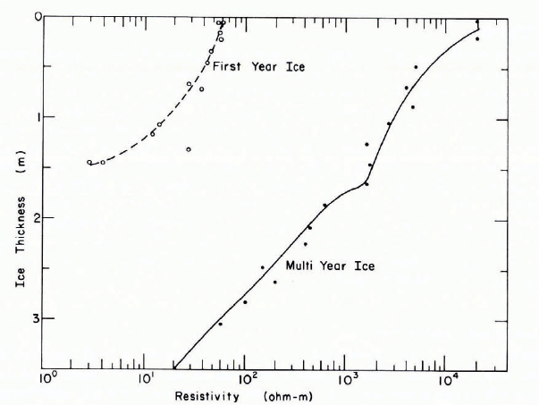
Fig. 15. Vertical resistivity profiles of typical first year and multi-year sea ice measured at 18.6 kHz (Reference McNeill and HoekstraMcNeill and Hoekstra, 1973.)

One rather surprising result of both the resistivity studies of McNeill and Hoekstra and of Kohnen is that when the electrode array was moved from site to site on the ice using a fixed electrode spacing and a similar lateral shift for each move, the apparent resistivity showed large fluctuations of a factor of four (see Fig. 16) even though the first-year ice in both areas was specifically selected for its apparent lateral homogeneity and each measurement integrates over a considerable volume of ice. These are rather sobering results, because if such variations prove to be commonplace in otherwise laterally uniform sea ice, they obviously must be considered in the development of remote-sensing systems designed to measure ice characteristics. These resistivity fluctuations must at least in part be due to erratic salinity variations. It has been known for some time (Reference Weeks and Lee.Weeks and Lee, 1962) that there are significant random lateral variations in salinity measured at identical depths in the ice. Even so, resistivity variations of such magnitude are surprising. Variations in multi-year ice would be expected to be even larger.

Fig. 16. The apparent resistivity of first year ice of uniform thickness determined in a linear traverse with a Wenner array having an electrode spacing of 0.92 m (Reference McNeill and HoekstraMcNeill and Hoekstra, 1973).

Studies of the dielectric characteristics of sea ice that cover a wide range of frequencies below 100 MHz and/or temperatures are those of Reference Wentworth and CohnWentworth and Cohn (1964), 0.1 to 30 MHz, —5 to —40°C; (Reference Fujino and ŌuraFujino 1967[a], Reference Fujino[b]), 100 Hz to 50 kHz, —5 to —70°C; Reference AddisonAddison (1969), 20 Hz to 100 MHz, —12.5 to —35°C; Reference KhokhlovKhokhlov (1970), 100 Hz to 1 MHz, —5 to —30°C; and Reference AddisonAddison (1975), 1 kHz, —25 to — 150°C. The studies of the temperature dependence of the dielectric constant, particularly that by Reference AddisonAddison (1975) have proven to be quite informative in that the temperatures at which the various solid salts crystallize from the brine can be identified. Also the data indicates the presence of brine within the ice until much lower temperatures (—70 to —75°C) than suggested by earlier studies. Finally, although there is evidence for fluoride doping in the ice phase of sea ice, there appears to be no strong reason for postulating substitutional chloride.

The measurements of the frequency dependence can be considered in three parts (Fig. 17). In the low frequency range both the real and imaginary parts of the dielectric constant (ϵ′ and ϵ″) show very large values (10⁴ to 10⁷) with ϵ″ values being larger than ϵ′ up to at least 1 MHz. The loss tangent (tan δ) is usually near 10 indicating that sea ice is a rather lossy material in this range. As frequency increases the values of ϵ′ decrease almost inversely up to 1 MHz. Reference AddisonAddison (1970) suggests that in this frequency range the observed electrical properties are principally controlled by the migration of ions in the irregular inter-connected brine channels that link the electrodes. The experimental observations (Reference Fujino and ŌuraFujino 1967[a], Reference Fujino[b]) suggest that at low temperatures when the brine channels are no longer interconnected, this mechanism becomes ineffective.

Fig. 17. Schematic diagram showing the variation in the real (ϵ′) and imaginary (ϵ″) components of the dielectric constant mid the loss tangent (tan δ) as a function of frequency; based primarily on results of Reference AddisonAddison (1969) and Reference VantVant (unpublished).

In the mid-frequency range (10 to 100 kHz), curves of ϵ′ versus temperature show a downward concavity and two maxima are observed in many of the tan δ curves. The suggested but tentative explanation is Debye dispersion of the ice protons with a somewhat shortened relaxation time. Similar reduced relaxation times have been observed in fluoride-doped ices.

At frequencies above 1 MHz the curves for ϵ′ flatten out and the ϵ″ curves also decrease less rapidly (above 10 MHz). There is also a gradual decrease in tan δ from 1 MHz to 10 MHz where it usually has values near or below unity. The dispersion in this range is believed to be the result of interfacial polarization arising from the presence of brine inclusions. As such, it should be possible to model the variations in ϵ in terms of a mixed dielectric model based on the volume of brine present in the ice. That this would be a profitable approach was shown by Reference Weeks and CurrieWeeks (1968) who took the Wentworth and Cohn data at 3 MHz, grouped the values according to structural ice type (normal sea ice, frozen slush) and plotted ϵ′ versus v_b. The result was two straight lines with distinctly different slopes.

The dielectric properties of sea ice at higher frequencies have been studied by Reference Hoekstra and CappillinoHoekstra and Cappillino (1971), 0.1 to 24 GHz; Reference Sackinger and ByrdSackinger and Byrd (1972), 26 to 40 GHz; Reference VantVant and Others (1974), 10 and 35 GHz, and Reference VantVant (unpublished), 100 MHz to 40 GHz. Values of ϵ″ range between 2.5 and 6.0 and 0.0 and 1.9 respectively. In correlating their data Hoekstra and Cappillino used with considerable success over a wide range of brine volumes a dielectric mixing formula proposed by Reference DeLoorDeLoor (unpublished). The relation was

where ϵ_s′ and ϵ_i′ are the real dielectric constants of sea ice and pure ice respectively and v_b is the relative volume of brine. The actual values obtained by Hoekstra and Cappillino are suspect because the structure of the artificial sea ice that they produced by flash freezing was probably not similar to the structure of natural sea ice. The model assumes that the brine inclusions are spherical. Reference VantVant and Others (1974) also used this relation to correlate their data and obtained good results for frazil sea ice (correlation coefficient r = 0.81) and for columnar sea ice (r = 0.90). For multi-year ice the correlation was lower (r = 0.57). They also used another model based on Wiener’s dielectric mixing formula which gave a higher correlation (r = 0.723) for multi-year ice and slightly lower correlations (r = 0.76 and 0.85) for frazil and columnar ice. This work has recently been greatly expanded by Reference VantVant (unpublished) who has also successfully used empirical dielectric mixing equations to predict the dielectric behavior of sea ice at any of the several frequencies he studied. He has also attempted to develop a general theoretical model that works over a wide frequency range. At present the theoretical and observed values are in reasonable argeement for first-year ice. The fact that results for multi-year ice show less than good agreement is believed to be the result of large variations in the amount of entrapped gas in the ice as well as of the very low overall salinities characteristic of such ice. A detailed discussion of Vant’s results is beyond the scope of this paper. However, his results are particularly encouraging in that the dielectric loss of sea ice at 1 GHz is a factor of 5 less than initially reported by Hoekstra and Cappillino. Figure 18 shows the trends of the frequency dependence of both the attenuation (dielectric loss) in dB/m and the attenuation distance (skin depth) in meters for first-year sea ice based on the experimental results of Reference AddisonAddison (1969) and Reference VantVant (unpublished). This figure is very informative in explaining the difficulty in developing an operational system for remotely determining sea-ice thickness: at low frequencies the penetration is good (low attenuation) but the resolution is poor (the wave length λ» ice thickness h) while at high frequencies the resolution is good (h » λ) but the penetration is negligible. The figure suggests that the best compromise between these two conflicting requirements would be found in the frequency range between 10 MHz and 1 GHz. In fact the Geophysical Survey Systems Inc. VHF impulse radar system which has proven to be effective in profiling sea ice (Reference Campbell and OrangeCampbell and Orange, 1974; Reference KovacsKovacs, in press) has a center frequency in this range (100 MHz). Soviet investigators have also bad success in profiling sea ice when working in this frequency range (Reference Bogorodskiy and Tripol’nikovBogorodskiy and Tripol’nikov, 1975; Reference Finkel’shteynFinkel’shteyn and others, 1975).

Fig. 18. Attenuation and attenuation distance versus frequency for electromagnetic radiation penetrating first-year sea ice.(Reference AddisonAddison, 1969; Reference VantVant, unpublished).

Finally we would like to note that Reference Campbell and OrangeCampbell and Orange (1974) while using the above-mentioned pulsed radar system to measure the thickness of sea ice have noted a marked change in the amplitude of the return from a vertically polarized signal when the antenna was rotated. This anisotropy has been observed in both first-year and multi-year ice with all first-year ice showing the effect and some showing it very strongly. Similar but less pronounced results were observed on multi-year ice. The effect was not noted on fresh-water ice. In some fast-ice areas the orientation of the maximum return remained roughly constant over distances of the order of kilometers. In other areas characterized by obviously rotated ice plates, marked changes in the orientation of the maximum occurred over distances of meters. It has been tentatively suggested that these effects are the result of a highly preferred crystal orientation in the lower portion of the ice sheet and the one check that was made suggests that the maximum return is received when the output field is oriented roughly parallel to the c-axis direction (normal to the platy substructure). These experiments and their interpretation are, as yet, hardly conclusive. Nevertheless, if they are correct they will provide a link between the observations mentioned in the first portion of this review detailing the increasing evidence for the existence of large domains of ice crystals with similar caxis orientations in the lower portions of thicker (> 1 m) fast ice and the fact, noted several times in our discussion of mechanical properties, that changes in crystal orientation correspond to large differences in observed strength.

Conclusions

In the above we have attempted to provide an introductory assessment of what is known about the engineering properties of sea ice by discussing its mechanical, thermal, and electrical properties. We have not quoted all the pertinent references but we have to the best of our knowledge mentioned all the major studies relating to this highly specialized field of study. Works that we have omitted should be readily locatable via the bibliographies in the referenced material. Because of space limitations we have been unable to discuss adequately differences in experimental results as related to differences in measurement techniques. We caution the reader against using any of the experimental values quoted here without thoroughly investigating the techniques used in making the measurements. In discussing the available results, we have tried to stress gaps and inconsistencies in the data base. Specific obvious examples are the conflicting results on whether both E and σ_f go to zero at high values of v (>0·3) or have values that are essentially independent of v_b This is particularly important inasmuch as the lower portion of every piece of sea ice contains ice that has brine volumes in or near to this range. Also important is the effect of variations in strain- or stress-rate, of sample size, of the loading direction in relation to the crystal orientation, and of the precipitation of solid salts within the ice.

There is clearly much to be done. However, we feel that if proper standardization of testing techniques is followed by combined laboratory and (when necessary) field testing, we should be able to resolve many of the remaining problem areas within a reasonable period of time. Writing this review has helped clarify many of these problem areas for us. We hope that it will serve as a similar aid to the reader. We anticipate that considerable advances will be made in our understanding of the engineering properties of sea ice within the next few years. It is certainly essential that such advances be made if the engineering problems associated with increased off-shore activities over the Arctic continental shelves are to be analyzed using good quality data as opposed to “informed guesses”.