


1. The Mechanical Properties of Ice
Present knowledge of the mechanical properties of ice suggests a re-examination of the theory of the flow of long valley glaciers. It has sometimes been assumed that ice under stress behaves like a very viscous Newtonian liquid: in other words, that for ice, as for a liquid, there is a proportional relationship between rate of strain (velocity gradient) ![]() and shear stress τ, as shown by curve B in Fig. 1 (p. 83), although the coefficient of viscosity for ice is much greater than for a normal liquid.Footnote * Unfortunately, this assumption, although mathematically simple, does not represent the real behaviour of ice very well. A constant viscosity is not observed with other polycrystalline materials such as metals, and it would be surprising if ice were an exception. In fact the matter seems now to have been put beyond doubt by careful laboratory experiments carried out by Mr.J.W. Glen.Reference Glen
11
He finds that, just as with a metal, applying a sustained constant stress (he actually applies a uniaxial compressive stress) to a specimen of ice causes it to deform permanently, and that after a few hours (the “transient” period) the rate of deformation settles down to a steady value. If the experiment is repeated with different values of the stress, the relationship between shear stress τ and the rate of shear strain
and shear stress τ, as shown by curve B in Fig. 1 (p. 83), although the coefficient of viscosity for ice is much greater than for a normal liquid.Footnote * Unfortunately, this assumption, although mathematically simple, does not represent the real behaviour of ice very well. A constant viscosity is not observed with other polycrystalline materials such as metals, and it would be surprising if ice were an exception. In fact the matter seems now to have been put beyond doubt by careful laboratory experiments carried out by Mr.J.W. Glen.Reference Glen
11
He finds that, just as with a metal, applying a sustained constant stress (he actually applies a uniaxial compressive stress) to a specimen of ice causes it to deform permanently, and that after a few hours (the “transient” period) the rate of deformation settles down to a steady value. If the experiment is repeated with different values of the stress, the relationship between shear stress τ and the rate of shear strain ![]() in the specimen is given by a curve of the general shape shown at A in Fig. 1 At low shear stresses the rate of strain is small; for higher shear stresses, however, the rate increases very rapidly, so that a small increase of stress produces a large increase in strain-rate. This is the type of curve, then, on which a theory of glacier motion should be based.
in the specimen is given by a curve of the general shape shown at A in Fig. 1 At low shear stresses the rate of strain is small; for higher shear stresses, however, the rate increases very rapidly, so that a small increase of stress produces a large increase in strain-rate. This is the type of curve, then, on which a theory of glacier motion should be based.
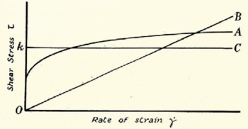
Fig. 1. Relations between the rate of strain ![]() and the applied shear stress τ: A, ice (after Glen); B, liquid of constant viscosity; C, simplified flow law used in section 4
and the applied shear stress τ: A, ice (after Glen); B, liquid of constant viscosity; C, simplified flow law used in section 4
In a glacier the state of stress is not uniaxial, as in Glen’s experiments, but triaxial, and in particular there is a hydrostatic pressure acting deep in the ice. The pressure reaches about 30 atmospheres in the Mer de Glace and 300 atmospheres or more in the Greenland ice cap. It has been suggested by Streiff-Becker, by Haefeli and by Demorest that this pressure may make the ice more deformable at depth, that is, reduce the shear stress needed to produce a given rate of strain. There seems to be no direct experimentaI evidence on the behaviour under shear stress of ice or any other polycrystalline substance already subjected to a high pressure and very near the melting point, and I think one should keep an open mind on what might occur. It may be remarked, however, that a pressure effect is not observed in metals far from the melting point, and that with liquids the viscosity is substantially independent of pressure. The present discussion is founded on the assumption that any pressure effect is negligible in ice. Should the existence of such an effect be later proved by experiment the necessary modifications of the expressions in Section 2 would be simple; the changes that would occur in the results of Section 3 are not so obvious. (See also Journal of Glaciology, Vol. 2, No. 11, 1952, p. 52–53.)
A possible effect of hydrostatic pressure on the shear stress necessary to produce a given rate of deformation should be distinguished from the diminishing slope of Glen’s curve A in Fig. 1. of this paper, which might be described as a lowering of viscosity with increasing shear stress.
For the purpose of calculation it is convenient to express curve A analytically. Glen finds that for polycrystalline ice with random crystallographic orientation a power law gives a good fit over the range of stresses τ = 0.8 to 5.5 barsFootnote *:
where B and n are constants. (This law was suggested by Perutz.Reference Perutz
2
) For ice at −1.5° C., if ![]() is expressed as shear strain per year and τ is in bars, B = 1.62 and n = 4.1, but the values of the constants depend rather sensitively on the amount of bubbliness in the ice and on the temperature. In this formula both τ and
is expressed as shear strain per year and τ is in bars, B = 1.62 and n = 4.1, but the values of the constants depend rather sensitively on the amount of bubbliness in the ice and on the temperature. In this formula both τ and ![]() are always to be taken as positive.
are always to be taken as positive.
2. Laminar Flow
A liquid of constant viscosity obeys the law (1) with the value of n = 1. With the more general flow law we are in a position to attempt a recalculation of the distribution of velocities within a valley glacier on the same lines as Somigliana’s calculationReference Somigliana 3 for n = 1.
The simplest case to start with is that of flow down a uniform plane slope (Fig. 2a , above). Axes are taken as shown, with the origin on the surface and Ox down the line of greatest slope. Oz is horizontal and perpendicular to the plane of the diagram. It is assumed for the moment that the lines of flow are everywhere parallel to the bed and that conditions are the same on all sections perpendicular to Ox. The shear stress on a layer at a depth d, which is measured perpendicular to the surface, is
where ρ is the density, assumed constant, g is the acceleration due to gravity and a is the angle of the slope. ![]() in (1) is here du/dy, where u is the velocity. It then follows, by integration, that the difference between the velocity u
0 of the top layer and the velocity of the layer at depth d is given by
in (1) is here du/dy, where u is the velocity. It then follows, by integration, that the difference between the velocity u
0 of the top layer and the velocity of the layer at depth d is given by
where ![]() .
.
The relative velocity between the top and bottom layers is thus
where u b and τ b are respectively the velocity and the shear stress on the bed, and h is the total depth measured perpendicular to the bed.
ϕ, the volume passing through any cross-section in unit time, for unit thickness in the z direction, is given by a further integration:

Fig. 2. Laminar flow down an inclined plane
One sees from equation (2) that if K, n, αand u 0 are given one can calculate the velocity at any required depth. For the physical problem, on the other hand, we may regard ϕ, K, n and α as given. Equation (4) does not enable h to be found, though, because u b is not yet determined. One could have the same for different values of h, as indicated in Fig. 2b (p. 83).
The physical properties of ice used in the calculation so far do not allow a prediction of how fast the glacier slips on its bed. All we can calculate are differential velocities within the ice. Therefore, on these assumptions, one cannot predict the depth of a glacier from a knowledge of its surface velocity and slope; the two cases indicated in Fig. 2c (p. 83), for instance, could not be distinguished. On the other hand it would evidently be possible to find an upper limit for the depth, and if ϕ were known as well as the surface velocity and slope, the depth could be deduced.
3. Effect of The Valley Sides
We now have to ask what effect the sides of the valley will have on these results. One may first notice that exactly the same equations (2), (3) and (4) apply to an infinitely deep, narrow glacier (Fig. 3, above), if the symbols are given the meanings:
-
u 0 = velocity on the central plane,
-
u = velocity at a distance d from the central plane,
-
u b = velocity at the edges,
-
α = slope of the surface, as before,
-
h = the half width.
K and n have the same meanings as before.

Fig. 3. Laminar flow in an infinitely deep channel of finite width. Plan view
A case intermediate between the very wide and the very narrow valley would be a bed formed from one half of a circular cylinder (Fig. 4, below). This is an easy problem to treat because the surfaces of maximum shear are all half-cylinders parallel to the bed. Simple statics shows that the variation of shear stress τ with depth is still linear but that the rate of increase is just half as rapid as with a very wide valley of the same slope. Thus
where r is the distance from the x axis of the point considered. Equations (2), (3) and (4) take the form.
R is here the maximum depth, the radius of the cylinder. The same remarks about the possibility of finding, from a knowledge of u 0, an upper limit to the depth, but not an exact figure, apply to this case equally.

Fig. 4. Flow in a channel farmed from a half-cylinder
Somigliana, treating the case with n = 1, was able to give an exact analytical solution for a bed whose cross-section formed a semi-ellipse, and he also made calculations for beds of more complex shape. Unfortunately, with the more general flow law (1) more complex cross-sections than a semicircle do not readily lend themselves to exact analysis. We therefore have to resort to approximate methods.
In a glacier of arbitrary but constant cross-section, flowing uniformly, one may find the average value of the shear stress, τ au , at the bed by simple resolution of forces. If the area of cross-section perpendicular to the bed is A and the perimeter of this cross-section is p, then, for unit length of valley, a force ρgA sin α due to the weight is balanced by a force τ au p due to the resistance of the bed. Therefore
(A/p is analagous to the “hydraulic radius” of a river valley or channel, but it should be noted that A and p are measured here not in a vertical plane but on a section perpendicular to the bed.) The values of A and p are not known for many existing glaciers. On the other hand, there are a number of glaciers whose depths are now known. Knowing the depth and width of a glacier one may make a good guess at the value of A/p. The procedure I have used (see also KoechlinReference Koechlin 4 ) is to put a parabola through the three known points, the lowest point on the bed and the two marginal points on the surface, to assume that the upper boundary of the cross-section is a horizontal line, and hence to calculate A/p. One also needs to know a. But in real glaciers the slope of the bed is not always the same as the slope of the surface. So which slope should be taken in the formula? The following argument makes it plausible that the surface slope is the right one to use. For fuller arguments leading to the same conclusion see reference Reference Nye5.
Consider a wedge-shaped block of ice whose surface has a slope a resting on a slope of inclination β (Fig. 5, p. 85). Provided (α − β) is small the shear stress acting on the bed at the point P may be approximately calculated. By the argument used for the parallel-sided slab, the shear stress at P a plane drawn parallel to the surface is ρgh sin a where h is the depth of P. Since the bed is near a plane of maximum shear stress, the shear stress on the bed itself will only differ from ρgh sin α by a small amount, particularly if (α − β) is small, since (α − β) is the angle through which one has to rotate the axes of reference of the stress tensor, α and not β is therefore the angle to be used.

Fig. 5. Diagram illustrating that the shear stress on the bed is ρgh sin α rather than pgh sin β, when (α − β) is a small angle
The calculation of τ au using the data for sixteen Alpine glaciers collected by Mercanton Reference Mercanton 6 gives values of τ au ranging from 0.49 bars, for the Unteraar Glacier at 2100 m. in 1945–47 (the last in the list), to 1.51 bars, for the Grenz Glacier at 2700 m. in 1948–49 (the fifth in the list). Considering the comparatively wide range of widths and depths involved and, particularly, the wide range of slopes, the spread of values of τ au is not very large—a result which might have been anticipated from the form of the curve A in Fig. 1.
One way of proceeding further is to assume that the linear variation of τ xy with depth that was found for a circular cylindrical bed and for a plane bed also holds for these more complicated cross-sections, and that the rate of increase of τ xy with depth on the central vertical plane z = 0 is fixed by putting τ b , the actual shear stress on this part of the bed equal to τ au , as is also rigorously true for the cylinder and the plane. This assumption gives a formula analogous to (3) for the relative velocity of top and bottom
In theory, therefore, knowing the value of u 0 one could predict the value of u b . The calculation is not very reliable because the flow may not be laminar, as discussed in the next section, because the assumption of linearity for τ xy may be at fault, because τ b may not be equal to τ au , and because the values of B and n are not yet precisely known for the temperatures and types of ice in the glaciers considered. Nevertheless, in spite of this formidable, and perhaps rather pessimistic, list of pitfalls, it is encouraging that when the calculation is made for the sixteen glaciers listed by Mercanton,with the values of B and n found by Glen for −1.5° C., the relative speeds of top and bottom always come out less than the observed surface velocities and give reasonable figures for the bottom velocities, ranging from 4 m./yr. for the Arolla Glacier at 2210 m. in 1908–9 (the second in Mer-canton’s list) to 79 m./yr. for the Rhône Glacier at 2520 m, in 1945–47 (the ninth in the list). If the calculation is done the other way round and used to predict an upper limit for the depth from the measured surface velocities, the calculated depth is always greater than the measured depth.
From this discussion one point stands out. No satisfactory answer, without ad hoc assumptions, seems to have been given to the question of what ultimately determines u b . But, until this question is answered, mathematical analysis may be able to explain the observed relative velocities within glaciers but it will not be able to predict at all the absolute velocities of movement. If u b was found in practice to be much less than u 0 the matter would be less serious. In fact this is by no means the case, and indeed it seems that sometimes the major contribution to the surface velocity comes from u b and only a small part from differential movement within the ice.
4. Compressive and Extending Flow
In Sections 2 and 3 attention was restricted to pure laminar flow, in which all points move parallel to the bed. In such a state of flow the surfaces along which shearing takes place, in a diferential sense, are in all places parallel to the bed. On the central vertical plane, assumed here to be a plane of symmetry, the stress components acting are τ xy , σ x , σ y and σ z (Throughout this paper tensile stresses are counted as positive.) τ xy increases linearly with depth and σ x =σ y =σ z = ρgy cos α − A, where A is the atmospheric pressure. The three normal pressures must be equal as they would otherwise cause a longitudinal or transverse extension or compression, which is contrary to the original assumption. The stress in the surface at z = 0 is therefore a pure hydrostatic pressure A. It follows that a pure laminar flow theory cannot include any explanation of transverse crevasses or shear faults on the central axis of a glacier.
To explain these phenomena we need to study a more complex type of flow in which an excess longitudinal stress is allowed. The mathematics of this are rather more complicated, and in the exact analysis a difficulty is met similar to that mentioned for laminar flow, namely that of postulating a suitable, and physically plausible, law to give the velocity or the shear stress on the bed. The difficulty is avoided, and the main features of the analysis are retained, if one assumes a simpler flow law. The one chosen is shown by curve C in Fig. 1. It is the special case of law (1) obtained by putting n infinite. This is equivalent to assuming that the rate of strain is very small up to a certain shear stress, k (≃ 1 bar), and that shear stresses greater than this do not occur. (For n infinite, B = k) As the flow theory based on this simplified law has already been published elsewhereReference Nye 7 the details will not be given here but only some of the results. It was assumed that the effect of the drag of the valley sides was negligible, as would be the case in a very wide valley. It seems Iikely, though, that the main results apply on the vertical axial plane of any valley glacier.
The analysis shows that there are two possible sorts of flow. One sort gives a longitudinal stress σ x which is compressive throughout the depth of the glacier (Fig. 6, above) and always more compressive than σ y ; the other gives a longitudinal stress which, although compressive at depth, is tensile in an upper surface layer, and is always more tensile (that is, algebraically greater) than σ y . The result is that in the first case the forward velocity of the glacier decreases as one goes down glacier, because the ice is being compressed, and in the second case the velocity increases because the ice is being extended. One could call the first case “compressive flow” and the second “extending flow.” (In the paper referred to above I used the terms “passive” and “active” flow, borrowed from soil mechanics, to describe these states. I think the new terms are preferable as being more graphic and less likely to lead to confusion.)

Fig. 6. Stress distribution in compressive or extending flow of a parallel-sided slab on a slope of angle a. In the figure a has been taken as cot−1 5 = 11.3°. This diagram differs slightly from the one given in reference Reference Nye7 in that the effect of atmospheric pressure has been included by moving the carves for σ x and σ y an amount A(≃ k) to the left
An immediate result is that one could expect transverse crevasses to form during extending flow but not during compressive flow. When the effect of atmospheric pressure is taken into account (which is strictly necessary because it is of the same order of magnitude as k) the theoretical thickness of the zone of tensile stress is approximately (2k − A)/ρg ≃ k/ρg ≃ 11 m., but of course this figure is only to be thought of as giving a rough approximation. Crevasses might be expected to open up to about this depth. Their presence would then modify the stress distribution and they might propagate to greater depths. On the wall of a crevasse at a depth 2k/pg ≃ 23 m., however, the pressure from above (A + 2k) would exceed the lateral pressure, A, by 2k, which is the yield stress in compression, and so below this the crevasse would close up comparatively rapidly.
Another distinction between the two types of flow can be made by considering the slip-line fields (Fig. 7, below). A slip-line field is represented by two families of curves drawn so that their directions at any point give the two perpendicular directions of maximum shear stress (that is, the two directions in which the tendency to shear is greatest). In both the present cases they are parallel and perpendicular to the bed at the bottom but they turn so as to emerge at 45 degrees to the surface. The curves are parts of cycloids, and the field in compressive flow is the mirror image of the field in extending flow. The importance of the slip-lines is that they show the directions in which the ice has the greatest tendency to fracture by shear. If the ice had no structure of its own one would expect that if shear fractures—faults—occurred, they would run along the directions of the slip-lines. Actually, of course, the ice is not equally strong in all directions and the laminar structure which every glacier possesses probably provides surfaces of weakness. One could say, therefore, that the closer any surfaces of weakness are to the slip-line directions, the more liable they are to give shear faulting.

Fig. 7. Slip-line fields and possible faults
In practice, by chance, the banding in glaciers often tends to run roughly the same way as one set of slip-lines (PP′ in Fig. 7) and this is probably why thrust planes are formed in glaciers with just about this shape. Shear displacement exactly along a slip-line would give the step shown at P′ in the figure. Faulting along the orthogonal set of slip-lines is not seen so often, nor is the corresponding faulting in the extending solution often observed. This may be because, first, it could be obscured on the surface by crevassing and, secondly, because the necessary slip-lines are not parallel to any structural surfaces of weakness. There may be a few examples of it however, such as the one shown in Fig. 6 of reference Reference Nye7.
In the calculations with the simplified flow law, unlike those for laminar flow, which were made with the more realistic flow law, it is possible to allow for the effect of accumulation and ablation, and also for changes in the slope of the glacier bed. In fact, which type of flow occurs, compressive or extending, depends on just these two factors. If ϕ is the rate of discharge, as defined in Section 2, dϕ/dx is the rate of addition of ice to the upper surface of the glacier. Positive dϕ/dx represents accumulation; negative dϕ/dx represents ablation. The second factor is measured by R, the radius of curvature of the bed. If R is positive the bed is convex, and if R is negative the bed is concave. The criteria for the two types of flow may then be expressed as:

Thus, if there were no changes in the slope of the bed, R would be infinite everywhere, and so where dϕ/dx was positive (accumulation area) extending flow would occur, and where dϕ/dx was negative (ablation area) flow would be compressive. At the other extreme, if there were neither accumulation nor ablation, dϕ/dx would be zero and it would then be the sign of R that decided the type of flow. A convex bed (R positive) would give extending flow, while a concave bed (R negative) would give compressive flow. In general, both factors are present; Fig. 8 (p. 90) shows the result expected in an idealized glacier valley. (The upper diagram in the figure shows the velocity distribution for the simplified flow law; for details reference should be made to the original paper.)

Fig. 8. Longitudinal section of an ideal glacier valley. The sign of R and the type of flow are given at the bottom of the figure. The lower diagram shows the slip-line field; the upper diagram shows the velocity distribution calculated with she simplified flow law C in figure 1
The following table summarizes the matter:

As mentioned at the beginning of this section, the theory just described, giving the two types of flow, is most easily developed for the simplified flow law with τ constant. But it can be shown that, by using the observed curve A, and making a suitable generalization to take account of the three-dimensional state of stress and deformation, the principal qualitative features of the simpler theory remain: in particular, the upper tensile layer and the general shape of the slip-lines.
I believe, therefore, that we ought to think of the flow of a glacier in a gently undulating, parallel-sided valley as a laminar flow of the simple type discussed in Section 2, to which is added a longitudinal extension or compression according to the curvature of the bed and according to whether there is accumulation or ablation at the surface. It is this last component of the motion that is related to the formation of thrust planes and transverse crevasses.
5. The Theory of Crevasse Patterns
The general explanation of the formation of crevasse patterns on glaciers was given in a fine paper by HopkinsReference Hopkins 8 in 1862, which must have been one of the first applications of the general analysis of stress to the distribution of stress in a continuously deforming body. The principles used in this section are essentially the same as those employed by Hopkins, except for the introduction of a result from the modern theory of plasticity. We neglect here the effect of atmospheric pressure, although strictly this is not permissible because its magnitude is comparable with that of the shear stress; the general effect of the pressure would be to reduce the area of crevasse fields. Let us first assume (Fig. 9, p. 91) that, if σ x is compressive on the surface of the glacier at the centre, it is also compressive, with much the same value, at other points of the surface right up to the margins; and, similarly, that there will also be regions where σ x at the surface is tensile with much the same value right across the glacier.

Fig. 9. The unbroken lines show the theoretical positions and directions of crevasses in three possible cases. The diagrams at the top indicate the stresses acting near the margin shown uppermost in the figure
If σ
x
is compressive the ice will tend to expand sideways in the z direction. There are two extreme cases to consider. If the sides of the valley are sufficiently steep to prevent lateral expansion a transverse compressive stress σ
z
will be set up, and the theory of plasticityReference Hill
9
shows that ![]() (both negative). Alternatively, the valley sides may be less steep and |σ
z
| would be less than this, or even zero. The same would be true if σ
x
were tensile: with steep valley sides transverse contraction by general downward movement might not be possible and a transverse tensile stress
(both negative). Alternatively, the valley sides may be less steep and |σ
z
| would be less than this, or even zero. The same would be true if σ
x
were tensile: with steep valley sides transverse contraction by general downward movement might not be possible and a transverse tensile stress ![]() would be set up at the surface; or, alternatively, σ
z
might be less than this and even zero. In all cases
would be set up at the surface; or, alternatively, σ
z
might be less than this and even zero. In all cases ![]() .
.
The only shear component of stress on the surface is τ
zx
This is zero at the middle and increases, in absolute magnitude, towards the margins. The result obtained (for instance by using the Mohr circle constructionReference Nádai
10
) when τ
zx
is added to the other components, σ
x
and σ
z
, is shown schematically in Fig. 9
a, b and c, p. 91. The lines show the direction of possible crevasses. They are drawn at all points where a tensile stress can exist. When σ
x
= 0 (Fig. 9b
) the principal axes of stress are everywhere at 45 degrees to the edge. One principal stress is tensile and the other is compressive, both being of magnitude |τ
zx
|; the tension, of course, decreases to zero at the centre. The effect of a longitudinal compressive stress (Fig. 9a
) is to swing the direction of maximum tensile stress more transverse to the line of flow, so that any crevasses would make angles of less than 45 degrees with the margin. The line of the crevasses should curve in the sense shown in the diagram, assuming σ
x
constant across the surface. The existence of a tensile stress in this case, however, depends upon rrizI reaching a certain value, and so the tendency to crevassing dies away towards the centre. If transverse expansion is prevented the necessary value of |τ
zx
| is ![]() .
.
A longitudinal tensile stress (Fig. 9
c) will swing the direction of maximum tension towards the line of flow. The crevasses would therefore meet the edges at angles greater than 45 degrees, and would curve across the glacier in the way shown. If, in this case, a transverse tensile stress (σ
z
) were developed, there would be a central strip of the glacier surface where both principal stresses were tensile. This can only happen at places where τ
zx
is not too large, and so the strip may not extend to the margins. If transverse contraction were prevented the condition for both principal stresses to be tensile would be ![]() . In this central strip one might expect to see crevasses not only transverse to the direction of flow but in many other directions as well; in particular, crevassing would be possible in the longitudinal direction, as indicated by the broken lines.
. In this central strip one might expect to see crevasses not only transverse to the direction of flow but in many other directions as well; in particular, crevassing would be possible in the longitudinal direction, as indicated by the broken lines.
A longitudinal compressive stress could be caused by ablation or a concave bed as discussed in the last section, or by a narrowing of the glacier valley, or on the inside of the bend when a glacier changes direction. In a similar way a longitudinal tension could be set up by accumulation, a convex bed, a widening of the valley or on the outside of a bend in the valley.
An examination of many photographs, including some hundred aerial photographs taken in Alaska by Mr. Maynard Miller, who was kind enough to lend them to me, shows that although crevasse fields are often highly complicated in their details the main features of many of them can be explained on the above Iines.
6. Acknowledgements
I should like to thank Mr. J. W. Glen for allowing me to use the unpublished results of his laboratory experiments on ice and I am also grateful to him and to Mr. W. V. Lewis for kindly reading and commenting on the first draft of this paper.
Appendix Profile of an Ideal Circular Ice Cap
OrowanReference Orowan 12 and HillReference Nye 7 have considered the quasi-static equilibrium of an ice cap resting on a horizontal base. They used curve C of Fig. 1 (p. 83) as an approximation to the plastic behaviour of ice and treated the case where the ice cap was very long in one horizontal direction, so that plastic spreading took place entirely in the other horizontal direction at right angles. In such an ice cap each half of the theoretical surface profile in the direction of flow is approximately part of a parabola. The equation is
where h is the height at a distance x from the nearer of the two edges; h
0 = k/ρg. If, k = 1 bar, h
0 = 11.3 m. and so ![]() , where distances are measured in metres. The equation does not hold very near the centre or the edges of the cap.
, where distances are measured in metres. The equation does not hold very near the centre or the edges of the cap.
It is interesting to consider what would happen if the two horizontal axes of the cap were comparable in length, and for this purpose we may take an ice cap that is circular in plan.
Consider the small prism-shaped element of such an ice cap shown shaded in plan and elevation in Fig. 10 (below). The prism, which is of height h, is taken to be at a distance r from the centre O of the ice cap. If the ice is spreading out radially there is an inward component of force exerted the floor on the base of the prism. If we assume a perfectly rough bed which exerts a coast shear stress k, the force is

Fig. 10. Ideal circular ice cap on a horizontal bed
If ![]() , as will be true except very near the edges of the cap, the normal pressure on the verticalfaces of the prism increases from approximately 0 at the surface to approximately ρgh at the base. The average pressure is thus
, as will be true except very near the edges of the cap, the normal pressure on the verticalfaces of the prism increases from approximately 0 at the surface to approximately ρgh at the base. The average pressure is thus ![]() . This results in a component of force acting radially outwards of
. This results in a component of force acting radially outwards of
The average pressure on the faces parallel and ,perpendicular to the radial direction may differ by an amount of order 2k, which would give an outward force of order 2khδrδθ. However, this is small compared with the term krδθδr, provided h ≪ r, and so we neglect it.
Equating the radial forces to zero and proceeding to the limit we find that, approximately,
where h 0 ≪ h ≪ r. This integrates to the parabola,
Where R is the radius of the cap, as the equation of the profile. The complete profile is thus part of the surface formed by rotating the parabola of Fig. 10 (p. 92) about a vertical axis through O. By comparing equation (A.3) with equation (A.1) we see that the profile taken through the centre of a circular ice cap of diameter 2R is identical with the transverse profile of a very long ice cap of width 2R.
It is perhaps surprising, at first sight, that the dimension transverse to the line of flow does not affect the profile, but the reason for this is clear when one considers a more general case.Reference Nye 13 It can be shown that the result just proved for a circular cap is merely a special case of a general theorem applicable to ice caps on uneven bases of irregular outline. The general theorem is that (1) seen in plan view, flow takes place in the direction where the downward slope of the surface is greatest; (2) the surface gradient α is connected approximately with the ice thickness h at each point by the equation
For the circular ice cap on a horizontal bed, ![]() , and equation (A.4) is identical with (A.2).
, and equation (A.4) is identical with (A.2).
For an ice cap of irregular shape resting on a horizontal bed the equation of the profile is evidently
where s is the distance from the edge taken along a line of flow. Equation (A.5) embraces both (A.1) and (A.3). The derivation of equation (A.4) and a discussion of its possible application to the Pleistocene ice-sheets and to Greenland arc given in reference Reference Nye13.


