
Introduction
There is broad consensus that decisions about what to conserve and how to do so are best made within a spatially-explicit framework of systematic conservation planning (Margules & Pressey, Reference Margules and Pressey2000; Groves et al., Reference Groves, Jensen, Valutis, Redford, Shaffer and Scott2002). The Landscape Species Approach is a framework developed by the Wildlife Conservation Society (WCS) to help conservation practitioners plan landscape-scale actions (Sanderson et al., Reference Sanderson, Redford, Vedder, Coppolillo and Ward2002). It centres around the careful selection of a suite of focal species, called Landscape Species, defined by their ability to represent all major habitats, management zones and threats at a site, their use of large, heterogeneous areas, and their structural and functional impacts on natural ecosystems (Coppolillo et al., Reference Coppolillo, Gomez, Maisels and Wallace2004).
Here we demonstrate the spatially-explicit steps of the Landscape Species Approach for addressing where and how much of the landscape or seascape to conserve and how to prioritize areas for action, including procedures for (1) mapping the attainable distribution (the Biological Landscape) of Landscape Species, (2) mapping varied human activities (Human Landscapes) and how those activities affect species, and (3) intersecting these Biological and Human Landscapes to create the Conservation Landscape, which in turn informs choices about conservation action relative to established goals. We illustrate this approach with case studies from the Adirondack Park, USA, and the San Guillermo-Laguna Brava Landscape, Argentina.
Methods
The Landscape Species Approach has been applied in whole or partly at 14 sites (Table 1), in 12 terrestrial and two marine seascapes. Hereinafter, we use landscape and seascape interchangeably. We first describe the general procedures of the approach and then specific applications and results for two case-study sites.
Table 1 Sites where the Landscape Species Approach has been fully or partially implemented.

The full framework of the Landscape Species Approach
To complete the Landscape Species Approach practitioners proceed through 10 steps (Table 2) reflecting systematic conservation planning (Margules & Pressey, Reference Margules and Pressey2000; Groves et al., Reference Groves, Jensen, Valutis, Redford, Shaffer and Scott2002). The approach's procedures for setting goals, selecting focal biodiversity, setting quantitative targets, and designing monitoring frameworks have been described in detail elsewhere (Table 2). This paper focuses on our procedures for compiling relevant spatial information, evaluating sufficiency of existing conservation areas, and prioritizing conservation action (steps 5–9). For each step, Table 2 references more detailed user manuals.
Table 2 The 10 steps of conservation planning using the Landscape Species Approach. The five spatially explicit steps (5–9) are described in detail here. The approach has so far been applied, in whole or part, in 12 terrestrial and two marine settings (Table 1). The user's manuals, produced by WCS's Living Landcapes Program (LLP), are available online (WCS, Reference Wilkie2009).
Selecting Landscape Species and setting Population Target Levels
Procedures for selecting Landscape Species are described in detail in Coppolillo et al. (Reference Coppolillo, Gomez, Maisels and Wallace2004) and Strindberg et al. (Reference Strindberg and Didier2006), and free software is available to assist practitioners. In brief, based on ecological information provided by users, the procedures help users select a complementary suite of focal species that efficiently represent all habitats, anthropogenic threats and management zones in a region. Table 3 provides an example suite of Landscape Species. The process is only meant to identify an efficient set of species-level focal features, although the relative efficiency of our procedures remains untested. The suite should help practitioners ensure their regions are large enough, sufficiently connected, and well configured to support functional populations of most species. Planners should also consider other types of focal features, including broader levels of biological organization (e.g. ecosystems, species assemblages), special elements (e.g. threatened, endangered, endemic species) and ecological processes (Groves, Reference Groves2003). Subsequent steps of the Landscape Species Approach can also be performed with these non-species features.
Table 3 Example of four Landscape Species and Population Target Levels in the Adirondack Landscape, USA. An assemblage of boreal bird species was also chosen but is not included here. Population Target Levels and the basis for determining those levels are preliminary and are being revised based on new information.
Quantitative targets for how many individuals of each Landscape Species practitioners aim to conserve are set according to guidelines in Sanderson (Reference Sanderson2006), and are henceforth called Population Target Levels. In brief, practitioners consider several levels at which they could conserve each species (such as demographic viability, ecological integrity, sustainable use, and historical levels) and then select a specific short-term target. Table 4 provides an example of the Population Target Levels for our two case-studies.
Table 4 Comparison of Population Target Levels to current, attainable, and future habitat capacity for Adirondack and San Guillermo Landscape Species, calculation of recovery and prevention targets, and adjustment of these for the impacts of current conservation. Units are numbers of individuals. All numbers should be considered preliminary and have not been subjected to review. Bold face indicates where an estimated capacity is below the Population Target Level. Each Landscape Species here reflects a slightly different conservation situation. In the Adirondacks, moose, loon, and bear primarily require actions to prevent future declines in abundance or at least, in the case of moose, maintain current habitat conditions so that the population can continue its recovery. Marten appear to need some recovery and preventative action, although estimates of current populations are being revised. In the San Guillermo Landscape conservation actions are being aimed at recovering populations, primarily by reducing poaching, especially as a way of buffering the populations against unavoidable future reductions caused by climate change and mining. In San Guillermo formal modelling of future human activities and their impacts on the distribution and abundance of Landscape Species has not been completed and, as a result, future habitat capacity and prevention targets have not been estimated.
* Estimates are currently being revised
Mapping the Biological Landscape
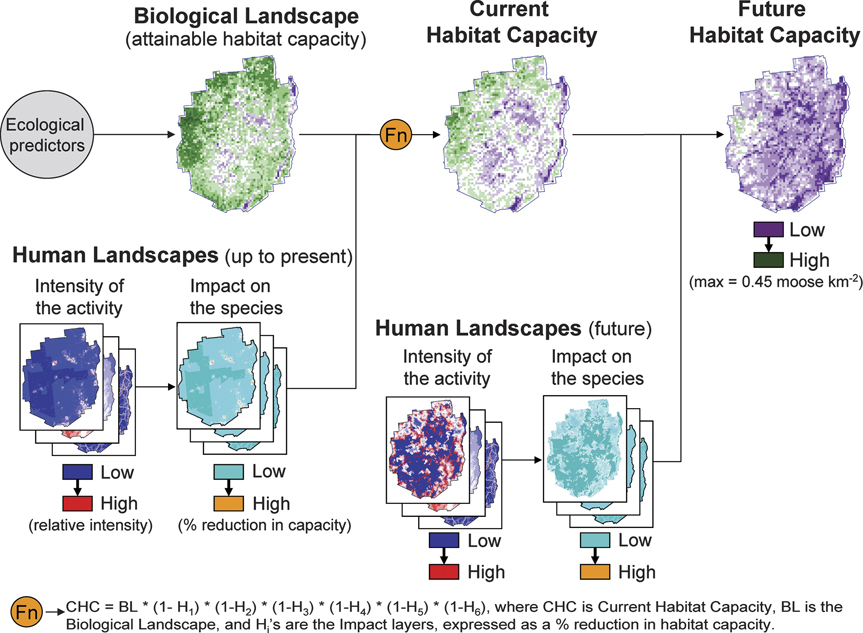
A Biological Landscape is a map representing the attainable distribution of a Landscape Species, i.e. what the distribution would look like if conservation action mitigated negative impacts of human activities (see Fig. 1 for an example). Biological Landscapes help practitioners: (1) envision how their region would look if conservation could recover populations to a more desirable state, (2) quantify recoverable population levels, and (3) provide one input for modeling the current distribution of the species. Often, Biological Landscapes reflect those human activities that conservationists feel cannot be mitigated (e.g. prior land-cover conversion) or choose not to mitigate (e.g. hunting by indigenous people). In this way, Biological Landscapes do not reflect unrealistic pristine states without human influence but more realistic conditions that conservation action could achieve.

Fig. 1 Overview of the modelling process for constructing Biological and Human Landscapes, and combining them, in this case for moose Alces alces in the Adirondack Park, USA. The Biological Landscape was modelled from a set of ecological layers and represents the attainable habitat capacity of the landscape if the impacts of human activities were mitigated. Human Landscapes were modelled representing the intensity of six human activities including land development (top visible layer), airborne pollutants (e.g. nitrate and phosphate deposition), hunting, logging, recreation and vehicular traffic on roads (i.e. road kill and habitat fragmentation). These intensity maps were then converted into maps reflecting the impact of these activities on moose up to the present time. The impact maps and Biological Landscape were then combined to make a map of the Current Habitat Capacity. The process was then essentially repeated, where the Current Habitat Capacity and future versions of Human Landscapes (i.e. one possible scenario) were combined to estimate a map of the Future Habitat Capacity. Note that the future pattern of land development in the Adirondacks is estimated to change substantially from the historical pattern.
The Biological Landscape, and all the distribution maps (e.g. current and future distributions), represent the species’ distribution at equilibrium with habitat conditions and do not attempt to account for source-sink dynamics, dispersal limitations or time lags in population growth. In this sense, it is appropriate to refer to them as habitat capacity (sometimes known as habitat quality or carrying capacity) maps, although our definition of habitat is broad. In addition to environmental and vegetation factors we also include in our definition and modeling those constraints imposed on a species’ distribution by other species (e.g. competition and predation). Henceforth, we use the terms habitat capacity and distribution models interchangeably.
In the majority of cases we use an expert opinion approach, as opposed to an empirical or statistical approach (e.g. multiple regression), to model Biological Landscapes (and Human Landscapes, below), similar to the US Fish & Wildlife Service's methods for creating habitat suitability models (USFWS, 1981). This is generally because empirical observations of the species in the landscape are not available or are of poor quality, and the only information available is what experts know or what has been published. Based on the best available information we identify life-long habitat requirements of the species and constraints on their distribution, including food, water, security and reproductive requirements, and biotic interactions. We then represent these factors with geographical information system (GIS) layers and weight individual factors according to their importance to the species, and combine them. The details for how habitat factors are mapped and combined differs substantially between species and landscapes, and is typically accomplished by comparing different options (e.g. adding vs multiplying factors) and using expert judgement. In rare circumstances sufficient direct observations of species are available, and statistical models can be built. In other cases so little is known about a specific Landscape Species (e.g. Andean cat in San Guillermo) that practitioners choose not to proceed with mapping until more information is available.
To facilitate comparison with Population Target Levels, Biological Landscapes are typically expressed in absolute abundance units (e.g. number of individuals, biomass), instead of relative abundance or presence/absence. Usually, models are built first in relative habitat scores and then translated to absolute units by estimating the density in areas with the highest habitat scores and linearly rescaling the values.
Mapping Human Landscapes
Human Landscapes help practitioners visualize where human activities occur and estimate how each activity affects species (see Fig. 1 for an example). Human Landscapes typically reflect the distribution and relative intensity of human activities (e.g. relative number of hunters, concentration of pollutants) as defined by Wilson et al. (Reference Wilson, Pressey, Newton, Burgman, Possingham and Weston2005). In these cases practitioners build expert opinion models by considering the factors structuring the activity (e.g. human population density, land cover types, road access). In some cases spatial data on mortality levels are available (e.g. fishing catch) and are used as Human Landscapes.
Practitioners are encouraged to map both past and future versions of Human Landscapes (Fig. 1). Past versions show the spatial distribution of human activities up to the present time, including recent impacts of ongoing activities. Future versions show forecasts of human activities.
After creating Human Landscapes, practitioners usually need to translate them into maps reflecting the impact of each activity on particular species (Wilson et al., Reference Wilson, Pressey, Newton, Burgman, Possingham and Weston2005). These Activity Impact maps may represent either direct reductions in populations (e.g. offtake from hunting) or indirect reductions through changes in particular habitat factors (e.g. forage availability reduced by fire), and are expressed as a percentage reduction in habitat capacity (e.g. each hunter removes a percentage of the local population) or an absolute reduction in habitat capacity (e.g. each hunter removes X number of animals, regardless of the population). Additional methodological details are available in Didier & LLP (Reference Didier2006, Reference Didier2008).
Mapping Current Distributions and Conservation Landscapes
By combining Biological and Human Landscapes practitioners can produce two additional maps: the species’ current distribution and a Conservation Landscape (see Fig. 2 for an example). The detailed analytical steps are described in Didier & LLP (Reference Didier2008). In brief, the current distribution map is typically created by reducing the attainable distribution (Biological Landscape) by the Activity Impact maps for the species. The exact combination process depends on the particular activity and how it is displayed in map form (e.g. as an absolute or percentage reduction). Current distribution maps can be compared with field measurements of the species’ distribution and abundance, although we expect that for several reasons (e.g. source-sink dynamics, population time lags) observed abundance will not always match habitat capacity. In a similar way, a future distribution map can be calculated by combining the current distribution with the future scenarios of Human Landscapes.
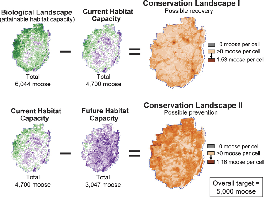
Fig. 2 Two versions of Conservation Landscapes can be produced using the Landscape Species Approach, as illustrated here for moose in the Adirondack Park, USA. By subtracting the current distribution from the Biological Landscape (attainable distribution), practitioners can produce a Conservation Landscape reflecting the potential for increasing populations through conservation action (i.e. recovery). By subtracting the future distribution from the current, they can produce a Conservation Landscape reflecting the potential for preventing future declines.
By simply subtracting the three different distribution maps from each other, practitioners can make Conservation Landscapes, which show the possible impacts of conservation activities across the study region. One version of the Conservation Landscape, created by subtracting the current distribution from the attainable (i.e. Biological Landscape), represents the potential to increase populations by mitigating past threats (i.e. population recovery). The second version, created by subtracting the future from the current distribution, reflects the potential for preventing decreases by mitigating future threats (i.e. preventable loss).
Assess sufficiency of existing conservation area and need for additional ones
Once the various Landscapes are created they can be used to assess the likely impact of planned activities and the need for additional activities. Because the Landscapes are expressed in units of abundance it is possible to sum across individual maps to generate estimates of a Landscape's attainable, current, and future total capacity to support the species. By comparing these different totals with Population Target Levels, practitioners can estimate a recovery target and prevention target. Four outcomes are possible (see Table 4 for an example): (1) The current and future habitat capacities for the species are above the Population Target Level, suggesting that little immediate action to reduce threats is needed; practitioners may wish to review the target level or focus on monitoring against new, unanticipated threats. (2) The current habitat capacity is above the Population Target Level but the future is below it, suggesting that conservation action should focus on preventing future threats. (3) The attainable habitat capacity is above the Population Target Level but the current and future are below it, suggesting that conservation action needs both to prevent future threats and mitigate impacts that have already occurred. (4) The attainable, current, and future capacities are all below the Population Target Level, suggesting that actions to mitigate both past and future threats are needed but also that the current extent of the Landscape needs to be expanded to reach target levels.
Prioritize areas for action
Conservation Landscapes provide valuable information for reaching conservation goals for Landscape Species. For example, it is possible to calculate the minimum extent of the Landscape needed to reach the target level for a particular Landscape Species simply by iteratively selecting areas with the highest possible recovery or prevention impact. To do the same across all Landscape Species would require optimization algorithms such as those in Marxan (Ball & Possingham, Reference Ball and Possingham2000).
However, Conservation Landscapes do not provide all the information one requires to set priorities of where to act or what actions to take. For example, Conservation Landscapes do not reflect costs of implementing conservation activities, practical constraints or opportunities that may limit or enable conservation action. In general, it is necessary to incorporate human judgement, often in a participatory setting, to identify spatial priorities for conservation action.
Although we have drafted methods for spatial priority setting these have not yet been satisfactorily tested in practice at a case study site. We envision inputting Population Targets for Landscape Species and Conservation Landscapes into decision support software such as Marxan (Ball & Possingham, Reference Ball and Possingham2000) or C-Plan (New South Wales NPWS, 2001). These software packages perform benefit-cost analyses to identify networks of conservation areas that efficiently meet quantitative targets for multiple biodiversity features, in our case Landscape Species. In the case of the Landscape Species Approach, Conservation Landscapes represent the benefits of conserving particular areas (i.e. preventing declines in population or recovering them; see example in Fig. 3). Although we have not fully explored how to represent costs within the approach, they can be represented as land area, estimated or observed monetary costs of implementing conservation actions, or opportunity costs. We envision producing maps that identify short- and long-term priority areas that change as information improves.
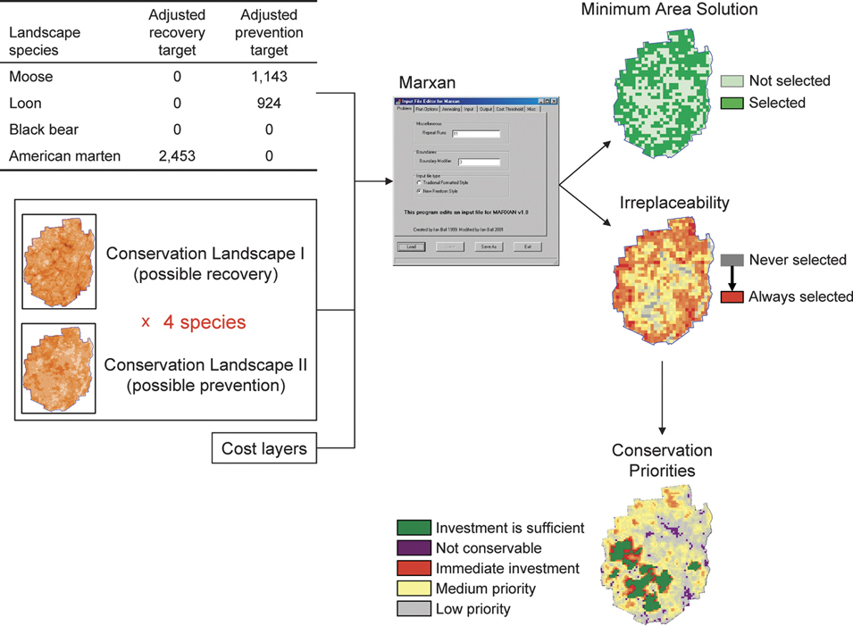
Fig. 3 Hypothetical example of our methods for spatial priority setting for the Landscape Species Approach for the Adirondack Park, USA. As these methods have not been field-tested, all maps are hypothetical. Targets, Conservation Landscapes and supplementary data (e.g. conservation cost) are input into conservation planning software, where practitioners can explore the optimal solutions and more realistic solutions based on additional information (e.g. connectivity, stakeholder input). Our goal is to produce a simple map of priorities, showing areas that are high priority for short-term investment and areas that are lower priority.
Case studies
Adirondack Park, USA
The Adirondack Park is a state park in the north-eastern United States in a transition zone between temperate and boreal forests. It encompasses 19,700 km2 in approximately equal proportions of privately-owned (mostly large areas managed for timber) and publicly-owned land (mostly large, roadless recreational areas). For a detailed description see Glennon & Porter (Reference Glennon and Porter2005). A Landscape Species suite for the Adirondacks was initially selected using an extensive participatory process during 2000–2003, subsequently revised, and now includes four species (Table 3) and an assemblage of boreal birds. Population Target Levels were set for this suite of species according to Sanderson (Reference Sanderson2006; Table 3).
Biological Landscapes were modelled for the suite of Landscape Species, as were six Human Landscapes. Fig. 1 shows examples of these for one species, moose Alces alces, and demonstrates how we combined Biological and Human Landscapes to produce a current distribution map. As local density estimates for moose were not available we based them on current densities from similar habitat in the state of Vermont. Both past and future versions of Human Landscapes were made but spatial patterns differed for only one activity, land development (Fig. 1).
These models illustrate that human activities have had a clear impact on moose habitat conditions up to the present, and may continue to degrade conditions into the future if not mitigated. Based on our Biological Landscape we estimate that the Adirondacks could support nearly 6,000 moose (i.e. the attainable habitat capacity), and that impact of human activities up until the present has reduced this by at least 1,300 such that current capacity is c. 4,700. Although our future landscapes represent only one possible scenario, they demonstrate that human activities could, over c. 25 years, further reduce capacity (by nearly 1,700 according to our model).
This example demonstrates that our distribution models represent habitat capacity and not necessarily observed abundance. Although current habitat capacity for moose is c. 4,700, the observed abundance is only c. 500 (NYSDEC, 2007). The moose population in the Adirondacks is recovering and has not yet reached the capacity of the current habitat.
We calculated Conservation Landscapes for each Landscape Species, representing the potential for recovering populations and preventing their future decline (Fig. 2). As moose populations will probably recover and exceed our population target (5,000) without intervention, conservation efforts are probably best focused on maintaining current conditions by preventing future declines in habitat. For moose, as for bear Ursus americanus and marten Martes americana, one of the greatest future threats comes from second home and infrastructure development. The future version of the Conservation Landscape illustrates that the impact of these is likely to be more severe on private lands, where land-use restrictions are weaker, unless conservation activities are implemented in these areas. Although we have not completed a prioritization of areas across all the Landscape Species, Fig. 3 illustrates our likely approach. In general, moose are reflective of other Landscape Species that we considered, in that they are faring relatively well, are probably viable and ecologically functional, but are threatened with declines in the future.
The Landscape Species Approach has had several implications for conservation in the Adirondacks. Firstly, the Landscape Species have received increased conservation attention and have been increasingly used in land-use planning, including increased protection of loons Gavia immer from pollutants such as lead and mercury, policy changes for back-country food storage and dramatic declines in human-black bear conflicts, and increased funding to monitor boreal birds and habitat. Conservation Landscapes have highlighted the possible impacts of proposed residential developments being considered by the local regulatory agency.
Secondly, by facilitating a participatory approach to planning conservation at a broad spatial scale, we believe the WCS Adirondack Program has increased its own visibility and ability to engage stakeholder and partners. For example, increased opportunities to collaborate with the New York State Department of Environmental Conservation and The Nature Conservancy were, in part, made possible because of their interest and engagement in these landscape-scale conservation planning activities. Finally, we believe that by encouraging the participation of both scientists and laypersons in a transparent, land-use planning effort focused on biodiversity, many stakeholders are more open to hearing arguments for conservation.
San Guillermo-Laguna Brava Landscape, Argentina
The San Guillermo-Laguna Brava Landscape is a remote, arid (150–450 mm annual precipitation) region, at 2,000–6,000 m, where the central Andean dry puna meets the southern Andean steppe and Argentine monte. It encompasses nearly 18,000 km2, is situated mostly within a UNESCO Biosphere Reserve, and includes a National Park and two provincial reserves. Because of its remoteness it is one of the most sparsely populated areas in the Southern Cone of South America, although as our analysis showed, human activities continue to have a negative effect on biodiversity.
In 2004 a suite of five Landscape Species were chosen with input from local stakeholders and scientists: guanaco Lama guanicoe, vicuña Vicugna vicugna, lesser rhea Rhea pennata pennata, Andean cat Leopardus jacobita, and the only native fish, pique Hatcheria macraei. Thus far, population target levels have been set for guanaco and vicuña, at 7,800 and 27,000, respectively, which are the estimated attainable capacities if threats are fully mitigated (Table 4). Targets for other species have not yet been set because of a lack of sufficient ecological information.
Biological Landscapes, past versions of Human Landscapes, and Conservation Landscapes (representing recovery options) were created for vicuña and guanaco. We demonstrate our modelling and planning using vicuña (Fig. 4). Density estimates in our spatial models were calibrated using other Argentine studies and information collected along transects. According to our models the current capacity of this Landscape to support vicuña has been reduced from c. 27,000 to 20,000 animals, primarily by poaching and livestock grazing in the southern portion of the Landscape, where the species has been extirpated, and in the Laguna Brava reserve to the north. Our models have also allowed us to simulate the possible impacts of other threats, including competition with introduced hares Lepus europaeus and local and downstream impacts of industrial-scale mining.
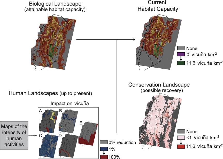
Fig. 4 Example of a Biological Landscape, Human Landscapes, Current Distribution map and Conservation Landscape, in this case for vicuña Vicugna vicugna in the San Guillermo-Laguna Brava Landscape, Argentina. The Human Landscapes showing intensity of the activities are not shown, only the impact maps relevant for vicuñas. They show the impacts up to the present time of (A) summer poaching (primarily from vehicles), (B) terrestrial impacts of mining, (C) competition from introduced hares, (D) hydrological impacts of mining, (E) livestock competition/poaching by herders.
The current population of vicuña in the San Guillermo-Laguna Brava Landscape is probably viable and ecologically functional. However, certain emerging threats, including increased aridity because of climate change and gold mining, could severely reduce vicuña abundances in the long-term. To buffer the population against these future threats, which are difficult to mitigate, our short-term population target (within the next 10 years) is to recover vicuña populations to the attainable capacity of 27,000, primarily by reducing poaching. Our models have helped determine where guard posts could prevent poaching and quantified possible impacts of planned mines.
Although the Landscape Species Approach has not been implemented in San Guillermo to the extent that it has in the Adirondacks, it has had several important implications for conservation practice. Firstly, unlike most other sites where the approach has been implemented, in San Guillermo it has been used since the initiation of our activities. It has helped us set basic project goals and select a manageable and logical set of species on which we can focus our limited resources. Our local partners and stakeholders are also interested in these Landscape Species, which helps us to draw these people into further discussions of the threats and their impacts.
Secondly, for the better known Landscape Species, guanaco and vicuña, the approach has helped us quickly to generate realistic, if imperfect, estimates of attainable and current populations and to demonstrate the impacts of threats. These estimates are powerful tools for convincing managers and other stakeholders that action is needed and can be effective. We are now able to indicate to managers that increasing ranger presence in key areas could increase the vicuña population by 30%, a more compelling argument than just saying that numbers could increase.
Thirdly, information produced through the approach has had clear impacts on management of the National Park and Biosphere Reserve. For example, data on poaching and its impact have been key in the recent re-establishment of the first permanent control outpost in the Biosphere Reserve. Finally, as in the Adirondacks, the participatory process involved in selecting Landscape Species and assessing human activities increased WCS's visibility and credibility in the region and, in turn, increased our network of collaborators, ability to involve stakeholders and, ultimately, our effectiveness in carrying out conservation in this Landscape.
Discussion
Innovations of the Landscape Species Approach
The conservation planning literature has long recognized the need to incorporate both the concept of representation (the ability of networks of conservation areas to include at least one occurrence of all biodiversity features) and biodiversity persistence into planning (Pressey et al., Reference Pressey, Cowling and Rouget2003). However, only recently have practical techniques emerged to consider persistence (Kerley et al., Reference Kerley, Pressey, Cowling, Boshoff and Sims-Castley2003; Early & Thomas, Reference Early and Thomas2007). The Landscape Species Approach explicitly incorporates the concept of persistence into its tools. Our procedures for setting quantitative targets encourage and help practitioners to estimate how large or dense populations need to be to ensure their long-term persistence and to maintain ecosystem services and ecological functions (Sanderson, Reference Sanderson2006). Biological, Human, and Conservation Landscapes, which are also expressed in abundance units, allow practitioners to compare spatial options directly against these quantitative targets.
Several studies have emphasized the importance of incorporating vulnerability (Margules & Pressey, Reference Margules and Pressey2000; Rouget et al., Reference Rouget, Richardson, Cowling, Lloyd and Lombard2003; Wilson et al., Reference Wilson, Pressey, Newton, Burgman, Possingham and Weston2005, Reference Wilson, Underwood, Morrison, Klausmeyer, Murdoch and Reyers2007). By mapping future human activities and estimating their possible impacts, our approach explicitly incorporates vulnerability into conservation planning. Within our framework, spatial priorities (step 9) should be guided, at least in part, by maps showing where future human activities may affect species. Therefore, the Landscape Species Approach weighs conservation priorities less on how much of a species’ current distribution can be included within reserves and more on the ability of a broader set of possible actions (e.g. anti-poaching patrols, community-based management) to minimize future losses. In this way our approach closely parallels the minimize loss approach of Pressey et al. (Reference Pressey, Watts and Barrett2004), the maximum-utilization framework of Davis et al. (Reference Davis, Costello and Stoms2006) and Wilson et al.’s (Reference Wilson, Underwood, Morrison, Klausmeyer, Murdoch and Reyers2007) approach, which measures the benefit of actions or areas as their ability to abate threats.
However, our methods for incorporating vulnerability have, thus far, been rudimentary and could be improved by considering several scenarios of future threats (business-as-usual, best-case and worst-case), and incorporating a measure of threat exposure, defined by Wilson et al. (Reference Wilson, Pressey, Newton, Burgman, Possingham and Weston2005) as either the probability that a human activity will occur in a particular area or the time until the area is affected. Exposure has been used in several studies (Margules & Pressey, Reference Margules and Pressey2000; Brooks et al., Reference Brooks, Bakarr, Boucher, Da Fonseca, Hilton-Taylor and Hoekstra2004) as a means for scheduling conservation action through time.
The counterpart of vulnerability to future reductions is the potential for biodiversity to recover and/or recolonize. By mapping past human activities and calculating what their impacts have been up to the present, the Landscape Species Approach also incorporates recovery potential, something that has typically been included only when restoration or reintroduction was an explicit goal or clearly necessary to reach targets (Kerley et al., Reference Kerley, Pressey, Cowling, Boshoff and Sims-Castley2003). Although many relatively intact places are primarily concerned with prevention, recovery of biodiversity is a realistic option in others (e.g. Walker et al., Reference Walker, Novaro, Funes, Baldi, Chehébar and Ramilo2004), and should be considered.
Challenges and new developments
Because empirical observations are unavailable or of poor quality (e.g. biased to a small part of the Landscape) in most cases we have taken an expert opinion approach to modelling the distribution of species and human activities. Recently, however, empirical approaches have been gaining wider use (Elith et al., Reference Elith, Graham, Anderson, Dudik, Ferrier and Guisan2006) and many can produce reasonably accurate spatial models with limited observations. The Landscape Species Approach could benefit from expanded use of empirical models but important practical questions remain regarding when empirical approaches should replace expert opinion. For example, when the number or quality of observations become severely limited (e.g. < 30 observations or severely biased observations) at what point, if any, does the accuracy of expert opinion models surpass that of empirical models? Or, when extrapolating models to other places or hypothetical conditions (e.g. attainable or future distributions), when and under what circumstances do expert-opinion models perform better than empirical models? Directed research could help practitioners make informed decisions about when to choose expert or empirical approaches.
Through our experiences at 14 sites we have identified three main improvements that could be made to the Landscape Species Approach. Firstly, our planning would benefit from a more rigorous estimation of cost. Although a few sites have attempted to map costs (in the Adirondacks, we used a simple expert-based estimate), we have not formulated a clear methodology for doing so. Although there is a strong case for planning based on benefits and costs (Newburn et al., Reference Newburn, Reed, Berck and Merenlender2005; Naidoo & Ricketts, Reference Naidoo and Ricketts2006) there is little consensus about appropriate cost measures. Approaches have included using land area, land purchase or easement costs (Newburn et al., Reference Newburn, Reed, Berck and Merenlender2005; Davis et al., Reference Davis, Costello and Stoms2006) and opportunity cost (e.g. Naidoo & Ricketts, Reference Naidoo and Ricketts2006). In our opinion, none of these concepts reflect well the costs of implementing conservation, which sometimes includes buying land but usually involves a much broader set of actions (e.g. enforcement, education, community-based management). Activity-specific accounting of costs, such as that used by Wilson et al. (Reference Wilson, Underwood, Morrison, Klausmeyer, Murdoch and Reyers2007) and Moore et al. (Reference Moore, Balmford, Allnutt and Burgess2004), is most appropriate but such information is rarely available and may itself be costly to collect.
Secondly, our approach has not explicitly tackled the challenge of maintaining or creating landscape connectivity. Connectivity considerations are probably best incorporated during the priority-setting step, when benefits of maintaining or increasing local subpopulations of species can be balanced against needs for connecting those subpopulations. Some decision-support software provides users with rudimentary tools for exploring connectivity options. For example, Marxan (Ball & Possingham, Reference Ball and Possingham2000) measures and manipulates compactness, a form of connectivity, using the perimeter of the network but does not formally select corridors. Other methods and software are specifically designed for identifying corridors among conservation areas, such as procedures using least-cost path concepts (Rouget et al., Reference Rouget, Cowling, Lombard, Knight and Kerley2006) or network flow (Phillips et al., Reference Phillips, Williams, Midgley and Archer2008). These need to be adapted for use in planning frameworks such as the Landscape Species Approach, and incorporated into other decision-support software.
Thirdly, it has become clear that our models cannot formally encompass all the important factors for priority setting and that stakeholders need to play a central role. Experts and stakeholders can informally incorporate many additional criteria, such as rapidly evolving political constraints (Meir et al., Reference Meir, Andelman and Possingham2004), identify major errors, and adjust decisions appropriately. Additionally, we have found that stakeholders who are not directly involved will often not trust or abide by resulting decisions. In practice, stakeholder participation has varied widely across the 14 sites. Sites have often first worked through steps internally and then, if they wished to influence external decisions, solicited feedback from larger audiences. More guidance is needed on how, when, and to what degree to include stakeholders, and how to ensure that recommendations are actually implemented (Marris, Reference Marris2007).
We asked our sites to estimate the time required to complete each step of the Landscape Species Approach. These estimates varied substantially among the eight responding sites (Fig. 5). On average, the entire approach required c. 1 year of person-time to complete (mean = 52 weeks, range 16–69), c. 60% of which was spent on the spatially explicit steps. The variation in these estimates is because of several factors, including the degree to which spatial data were compiled, the knowledge of species' ecology, human activities and GIS, and the degree of stakeholder participation. Also, many early applications of the approach included a substantial amount of time developing the tools. Now that development is mostly complete, application time should be reduced to 4–10 months, depending on the above factors.
Fig. 5 Time investment for the Landscape Species Approach based on a survey of eight sites. Sample size is < 8 for certain steps. Bars indicate maximum and minimum.
Looking broadly across all sites that have implemented the Landscape Species Approach, we believe there are three common advantages. Firstly, it has helped practitioners envision how to scale-up their conservation from small areas (usually parks or protected areas) to more biologically meaningful landscapes where human uses dominate (Sanderson et al., Reference Sanderson, Redford, Vedder, Coppolillo and Ward2002). The approach helps conservationists define the spatial extent and configuration of conservation areas that are needed for the long-term preservation of Landscape Species and, through these, functioning communities and ecosystem services. For example, in another of our 14 sites, the Madidi Landscape in Bolivia, practitioners realized they initially underestimated the landscape extent necessary to support particular species (e.g. jaguar Panthera onca) and are currently pursuing opportunities to expand their conservation efforts accordingly.
Secondly, the Landscape Species Approach helps practitioners create visual and quantitative products that make a powerful conservation argument. We suspect that, prior to seeing the results, many stakeholders do not realize that their ecosystems once supported substantially larger populations, nor the changes that future human activities may bring. For example, the approach in Glover's Reef Atoll, Belize, revealed that populations of queen conch Genus species and other species are an order of magnitude lower than that required for sustainable fishing. As a result, the Glover's Reef Advisory Committee is working with WCS to establish management mechanisms to recover the reef's biodiversity.
Finally, the Landscape Species Approach helps introduce biodiversity conservation concerns into land-use planning that is otherwise focused only on human livelihood concerns. For example, after participating in the approach for the Nam Kading Landscape in Lao PDR, government representatives began to incorporate wildlife objectives into their own planning, in addition to development and poverty alleviation objectives.
Acknowledgements
Many people have contributed to the development of the Landscape Species Approach, all of whom we cannot list here. We thank all WCS staff associated with the 14 landscapes listed in Table 1 and in the Living Landscapes Program, in particular Erika Reuter who edited an early version of this article. The development of the approach was made possible through the generous support of the United States Agency for International Development's Global Conservation Partners (USAID-GCP) Program, specifically through a Leader with Associates Cooperative Agreement Award LAG-A-00-99-00047-00. This article was made possible with additional USAID-GCP funding under Associate Cooperative Agreement Award EPP-A-00-03-00023. The contents are the responsibility of the authors and do not necessarily reflect the views of USAID or the United States government.
Biographical sketches
Karl Didier's interests include spatial ecology and modeling, conservation planning, and temperate grassland and tropical forest conservation. Michale Glennon's research interests include land use management and its relationship to biological diversity and integrity in the Adirondack Park. Andrés Novaro's areas of research include landscape effects on hunting, guanaco-puma interactions, and the migratory process in guanacos. Eric Sanderson's interests are in developing sustainable relationships between humanity and the rest of nature at all scales. Samantha Strindberg provides technical support in both strategic conservation planning and statistical design and analysis, especially focusing on the adaptation of existing techniques to deal with the challenges of monitoring wildlife. Susan Walker's research on landscape connectivity is being applied to the development of the Payunia-Auca Mahuida Guanaco Corridor in northern Patagonia. Sebastián Di Martino participated in the work here as a consultant for WCS, and is currently the Director of Protected Areas for the province of Neuquén, Argentina.