


1. INTRODUCTION
Precise Point Positioning (PPP) has become a major research area in the Global Positioning System (GPS) community as it could provide an accurate positioning service at a large-scale without the support of dedicated reference stations (Bisnath and Gao Reference Bisnath and Gao2007; Kouba and Héroux Reference Kouba and Héroux2001). It has been demonstrated to be a powerful tool in geodetic and geodynamic applications (Zumberge et al., Reference Zumberge, Heflin, Jefferson, Watkins and Webb1997; Kouba and Héroux Reference Kouba and Héroux2001; Gao and Shen Reference Gao and Shen2001; Zhang and Andersen Reference Zhang and Andersen2006). However, traditional PPP needs a long convergence time to achieve centimetre-level accuracy, so its application in rapid and real-time positioning is presently limited (Bisnath and Gao Reference Bisnath and Gao2007; Li et al., Reference Li, Zhang and Ge2010).
In order to shorten the convergence time and improve accuracy, several approaches for fixing integer ambiguities in PPP solutions have been developed in recent years. In the approach by Gabor and Nerem (Reference Gabor and Nerem1999), Single-Differenced (SD) Uncalibrated Fractional Offsets (UFOs) between satellites are used for removing the fractional part in SD ambiguities at the user for integer ambiguity fixing, based on their simulations. Ge et al., (2008) demonstrated the high spatial and temporal stability of the satellite UFOs and presented an approach to estimate the fractional parts of the SD UFOs between satellites from a global reference network. Results showed an improvement of about 27% in the repeatability and 30% in the accuracy of the east component. Laurichesse et al., Reference Laurichesse, Mercier, Berthias and Bijac(2008) introduced another approach, in which ‘integer’ satellite clocks are estimated from a network, in order to fix the dual-frequency GPS ambiguities of undifferenced phase measurements. After applying such integer clocks in PPP, the resulting positioning precision is comparable to that of standard differential positioning. Collins et al., (Reference Collins, Lahaye, Hérous and Bisnath2008) proposed a ‘decoupled clock model’, in which two sets of independent satellite clocks for phase and code respectively are used, requiring no assumption about the stability of code or phase biases. Although the above-mentioned approaches are realised in quite a different way, a comparative study (Geng et al., Reference Geng, Meng, Dodson and Teferl2010) confirmed their theoretical equivalence; thus we concentrate on the approach using UFOs instead of ‘integer’ clocks.
The UFOs are usually derived from the estimated Zero-Differenced (ZD) ambiguities. In the approach by (Ge et al., 2008), all possible SD ambiguities are formed for each satellite pair. Their fractional parts should be statistically the same if the ZD ambiguities are estimated precisely, as further difference between any two of them forms a Double-Differenced (DD) ambiguity, which should be very close to an integer. By taking the mean of the fractional part of the SD ambiguities of the same satellite pair over all the stations, the SD UFO is estimated.
In this study, instead of estimating a SD UFO for all satellite pairs, we present a new approach; ZD UFOs are estimated in an integrated adjustment together with sequential integer ambiguity fixing in order to enhance the estimates. The approach can be applied to both Wide-Lane (WL) and Narrow-Lane (NL) combinations if the corresponding ZD ambiguities are available. It does not matter whether the NL ambiguities of the reference stations are derived from PPP or network modes. Using NL ambiguities from PPP enables the UFO to be estimated from a network that is much denser than that necessary for the time-consuming task of clock estimation (Zhang et al., Reference Zhang, Li and Guo2010).
After a short introduction to the related mathematical background, the new approach is presented in detail. The algorithm for estimating UFOs from reference networks and applying them to a single station is described. Then, the new approach is evaluated for a variety of applications using several sets of data. The results of the validation are then presented and discussed.
2. ZD OBSERVATION MODEL
GPS ZD pseudo-range and carrier phase equations can be expressed as follows (Teunissen and Kleusberg, Reference Teunissen and Kleusberg1996):
where:
superscript ‘k’ refers to a given satellite.
subscript ‘i’ refers to the receiver.
t is the time when the signal is received.
τ ik is the signal travel time between the satellite and receiver antenna phase centres.
ρ is the geometric distance between the receiver and satellite antenna phase centres, at the signal reception and transmission times, respectively.
I ik is the ionospheric delay on the path.
T ik is the tropospheric delay on the path.
c is the speed of light.
dt i is the receiver clock correction at the signal reception time.
dtk is the satellite clock correction at the time of signal transmission.
d i(t) is the signal delay from the receiver antenna to the signal correlator in the receiver.
dk(t−τ ik) is the signal delay from the satellite signal's generation to its emission from the satellite antenna.
e ik is the pseudo-range measurement noise.
δ i(t) is the carrier phase signal delay from the receiving antenna to the signal correlator in the receiver.
δk(t−τ ik) is the carrier phase signal delay from the satellite signal's generation to its transmission from the satellite antenna.
λ is the wavelength.
φ i(t 0) is the initial phase of the receiver at the reference time t 0.
φ k(t 0) is the initial phase of the satellite at the reference time t 0.
N ik is the integer ambiguity.
ε ik is measurement noise of carrier phase observations.
By examining Equation (2), one can find that the float items of φ k(t 0), φ i(t 0), δk(t−τ ik), δ i(t) are also ambiguous. In the traditional standard PPP model (Kouba and Héroux Reference Kouba and Héroux2001), these items will be treated as ambiguities. Therefore, the ambiguities in the traditional standard PPP model lose their integer property. They have to be estimated as float values. It is worthwhile noting that the choice of analysis strategy and algorithm in the traditional standard PPP model results in ambiguities being estimated as float values. In the next section, an Integer Ambiguity Resolution method on the ZD level will be developed.
3. ZD INTEGER AMBIGUITY RESOLUTION
As the initial phases and hardware delays in Equation (2) are not easily separated, we can group them as uncalibrated phase offsets: b i for the receiver and bk for the satellite (Blewitt Reference Blewitt1989; Hatch Reference Hatch1996; Hofmann-Wellenhof et al., Reference Hofmann-Wellenhof, Lichtenegger and Collins1992). The non-dispersive items in Equations (1) and (2), such as geometric distance, troposphere etc., can be grouped together into ρ g. Then Equations (1) and (2) can be simplified:
where:
and we define:
where:
N ik is the integer ambiguity.
b i is the receiver-dependent uncalibrated phase delay.
bk is the satellite-dependent uncalibrated phase delay.
B ik is the comprehensive ambiguity without an integer property.
By examining Equation (7), one can find that the ZD ambiguity is contaminated by b. Generally, b is assumed to be slowly varying with time. However, the ambiguityB is considered as a constant and the receiver clock offset varies from epoch to epoch in GPS data processing. Consequently, the time-varying portion of b will be mostly absorbed by the clock and the constant portion of b will be absorbed into the ambiguity B. In addition, as code measurements are introduced into the PPP model, the group delay biases d will also contribute to the ambiguity estimation. Generally, group delay biases d vary slowly enough to be considered as constant over a short time interval (Gabor and Nerem, Reference Gabor and Nerem1999). Therefore, contributions from b and d to the ambiguity could be assumed as float constant offsets in a short time interval. The constant offsets have an integer part and a fractional part. The integer part is difficult to separate from the original ambiguity N. Fortunately, the integer part will not make the ambiguity lose its integer property. The integer property of ZD ambiguity is destroyed by the fractional portion (i.e., the UFOs). To enable Integer Ambiguity Resolution on ZD observations, UFOs need to be separated from B.
The following part will show the method used to separate UFOs from B in order to recover the integer property of the ZD ambiguity. We can reform Equation (7) as follows:
where:
B denotes float ZD ambiguities in the standard model.
Ñ denotes the sum of Nand the integer part of b.
f i denotes the UFO of the receiver.
fk denotes the UFO of the satellite.
In order to remove ionospheric delays, ionosphere-free observations (signal frequency L3) are usually used for the estimation of orbits and clocks and for PPP on the user side. The ambiguity of ionosphere-free combined observation (L3) can be expressed as follows:
where:
λ L3 is the wavelength of ionosphere-free combination (∼6 mm).
B L3 is the ambiguity of ionosphere-free combination.
c is the speed of light in a vacuum.
f L1 and f L2 refer to the signal frequencies of L1 and L2.
B L1 and B L2 are the ambiguities of L1 and L2.
Therefore, ambiguity resolution has to be conducted first in Wide-Lane (WL), and then in Narrow-Lane (NL). An L3 ambiguity is fixed as soon as both the WL and NL ambiguities are fixed. The WL ambiguityB WL can be calculated simply by taking the time average of the ‘M-W’ (Melbourne and Wübbena) combination (Melbourne Reference Melbourne1985, Wübbena Reference Wübbena1985) of the dual-frequency phase and range observations. The NL ambiguities are derived from Equation (9) with the already fixed WL ambiguity and the L3 ambiguity of the float ionosphere-free solution.
To recover the integer nature of ambiguities at a single station, the WL and NL UFOs must be estimated from the reference network and then provided to users as soon as the ZD ambiguities of the reference network are available.
4. ESTIMATION OF THE ZD UFOs
Let us assume that we have a network of ‘n’ stations tracking ‘m’ satellites. The float ZD ambiguities at each station are estimated as b i. For each ZD ambiguity we have an observation Equation (10) in the form of Equation (8):
where:
n i is the ZD integer ambiguity vector for station i.
f r and fs are the UFOs for receivers and satellites respectively.
R i and S i are the coefficient matrices for receiver and satellite UFOs respectively.
Q is the covariance matrix of the ZD float ambiguities.
In matrix R i all elements of one column are 1 and all other entries are zero. For matrix S i each line has one element of -1, the other entries are zero.
Obviously, we cannot estimate the integer ambiguities and the UFOs simultaneously because the number of parameters are m+n more than the number of pseudo-observations. Even if we knew all the integer ambiguities, there would still be a rank deficiency of 1. That means we have to fix one of the UFOs to, for example, zero.
Under the condition that all the integer ambiguities are known exactly and that one UFO is fixed to zero, then the UFOs can be estimated by means of a least square adjustment from the following observation Equation (11):
The ZD ambiguities must be estimated very precisely, so that their DD ambiguities are very close to integers. Otherwise, they cannot be used to derive UFOs. We assume that the UFO at the first arbitrarily selected station is zero. Then the nearest integers of the ZD ambiguities at this station are the integer ambiguities and the fractional parts are estimates of the corresponding satellite UFOs. When applying these satellite UFOs to the common satellites of the next station, the corrected ZD ambiguities should have a very similar fractional part. Of course, we can take the fractional part of one satellite as the UFO of the receiver. However, the mean fractional parts of all the common satellites, with proper quality control, give a better estimate of the receiver UFO. With this UFO, UFOs of the newly appearing satellites at the station can be estimated. Repeating this procedure for all stations, we can obtain the approximate UFOs for all receivers and satellites.
After correcting the ZD ambiguities with the UFOs, they should be very close to integers, thus ambiguity-fixing can be attempted. Replacing integer ambiguity parameters with their fixed values in Equation (10), the remaining parameters can be estimated. The UFO estimates are improved and will in turn help to resolve more integer ambiguities. The above procedure can be done iteratively until no more integer ambiguities can be fixed. The UFOs from the last iteration form the information needed by the user side for PPP ambiguity fixing.
The number of the fixed ambiguities contributing to a UFO parameter can be a very efficient indicator for use in quality control. From Equation (8), if an ambiguity cannot be fixed to an integer, the corresponding observation will not contribute to the estimation of UFOs at all. Therefore, satellite UFOs with contributions from few stations should not be disseminated to users, although the strategy does not require that all ambiguities must be fixed.
Based on the above UFO estimation approach, we developed a computational procedure for the estimation of UFOs on the server side and for using the UFOs for PPP on the user side. These are described in detail below.
First, we carry out a PPP float solution with International GNSS Service (IGS) orbit and clock products for all stations of the reference network with fixed station coordinates. The float WL ambiguities are estimated from the MW combination and the ionosphere-free ambiguities are estimated from the PPP solution. Then the approach in Section 4 is applied to all the float ZD WL ambiguities, so that the WL UFOs and integer ZD WL ambiguities are estimated. With the integer WL ambiguities estimated, the NL ambiguities are derived from the ionosphere-free ambiguities. Afterwards, the same approach is used to estimate the NL UFOs from the float NL ambiguities. Finally, we can offer the estimated WL and NL UFOs of satellites to PPP users together with IGS orbit and clock products, so that PPP with integer ambiguity fixing can be performed at a single station. The float WL and NL ambiguities are estimated in the same way as for the reference stations. Their satellite UFOs are removed by the estimated corrections, whereas the receiver UFO can be assimilated into the receiver clock by forcing one ZD ambiguity to its nearest integer. Afterwards, the ZD ambiguities have an integer property, so they can be fixed by making use of the same methods for fixing DD-ambiguities, such as the sequential ambiguity-fixing strategy (Dong and Bock, Reference Dong and Bock1989) or the LAMBDA method (Teunissen, Reference Teunissen1995). The detailed algorithm procedure, including the estimation of UFOs on the server side and PPP with integer ambiguity fixing on the user side, is shown in Figure 1.

Figure 1. Data processing procedure for estimation of UFOs from a reference network and their application to a single station for PPP with integer ambiguity fixing.
In the above UFO estimation method, the estimated UFO will change slowly with time due to the inaccurately modelled atmospheric delays and the multipath effect, etc. The NL UFO estimation is more likely to be adversely affected because of its short wavelength. Although pseudo-range noises will be introduced into the WL ambiguity estimation, WL UFOs are often more stable over time because the WL combination has a relatively long wavelength. Generally speaking, WL UFOs can be estimated every day and used for real-time applications with a long update interval. On the other hand, NL UFOs need regular estimation with short update intervals (especially for receiver UFOs). For example, the method can estimate a group of UFOs every few minutes (10 minutes for all examples in this paper), and make short-term predictions of NL UFOs for real-time applications. We used the observations from a tracking network shown in Figure 4 during Day Of Year (DOY) 121–130 (30 Apr–9 May) in 2008 to estimate WL UFOs every day and NL UFOs every 10 minutes as shown in Figures 2 and 3, in which all 144 groups in day 122 are shown. One can find that WL UFOs are rather stable and can be predicted for a long time. NL UFOs are also relatively stable in the short term but can only be predicted for a short time.
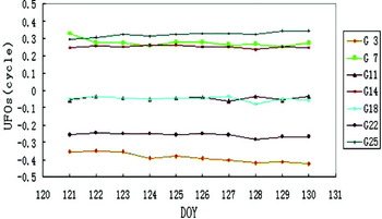
Figure 2. WL UFOs of satellites.

Figure 3. NL UFOs of satellites.
5. VALIDATION EXPERIMENTS
In this section, to validate the proposed method, examine its feasibility, and evaluate positioning accuracy, we conducted experiments at stations both in static and kinematic positioning modes and the float and fixed solutions were then compared.
5.1. Experimental Deployment and Data Processing Strategy
We used three networks: a local Chengdu ‘Continuous Operation Reference Station’ (CORS) network with an average station spacing of 40 km, the regional network of China with an average station spacing of 1200 km, and a continental network of IGS tracking stations with an average station spacing of 2500 km. These networks were used by the server to compute the UFOs to be applied to correct the ZD carrier phase measurements at the user. In the following sections, the distance between the PPP user and the network refers to the distance from the user to the closest station of the network. We name this the user-to-network distance. The three experiments with differently sized networks will be used to investigate the influence of network station density on the ZD ambiguity fixing rate and positioning accuracy. The details of these networks are described as follows:
• Experiment A. Stations inside China were chosen to make up the server-end of the observation network. The location of the network stations is shown in Figure 4, in which the ten blue solid circles represent the stations used to compute satellite UFOs. These stations are distributed approximately evenly across China with an average station spacing of about 1200 km. The green solid triangles represent the PPP user stations, of which three stations are located inside the network and nine stations are outside the network, in order to test the feasibility and accuracy of the method proposed in this paper. The designed user-to-network distance ranges from 800 km to 3000 km.
• Experiment B. IGS tracking stations outside China were chosen to make up the server-end of the observation network. The distribution of the network stations is shown in Figure 5, in which the ten blue solid circles represent the stations used to compute satellite UFOs. These stations are distributed from latitudes 14° North to 68° North and from longitudes 5° East to 142° East. Average station spacing is about 2500 km. The green solid triangles represent the PPP user stations to test the feasibility and accuracy of the method. The designed user-to-network distance for this experiment ranges from 800 km to 2500 km.
• Experiment C. The local Chengdu CORS network was chosen to make up the server-end of the observation network. As CORS networks already exist in many cities worldwide, we designed this experiment to test the feasibility of augmenting PPP with CORS, which would supplement the shortage of existing stations in DD RTK networks (in which RTK services are only available within an area around tens of kilometres from the network). The distribution of the network stations is shown in Figure 6, in which the six blue solid circles are the Chengdu CORS stations used to compute satellite UFOs. Average station spacing is about 40 km. The green solid triangles represent the PPP user stations used to test the feasibility and accuracy of the method. The designed user-to-network distance for this experiment ranges from 1200 km to 3500 km.

Figure 4. Network deployment of Experiment A.

Figure 5. Network deployment of Experiment B.

Figure 6. Network deployment of Experiment C.
Observation data from GPS week #1477 in 2008 was used for the three experiments. Precise orbit and clock products were downloaded from the IGS website. On the service-end, a set of WL UFOs was estimated every day, while a set of NL UFOs was computed every 10 minutes. The observations from user stations were separated into sessions of 30 minutes. PPP fixed solutions and float solutions were then conducted in static mode. IGS products (SINEX and TRO files) were taken as the truth for comparison. The LAMBDA method was employed to calculate the ZD integer ambiguity, and partial ambiguity resolution technology (Teunissen et al., Reference Teunissen, Joosten and Tiberius1999) was applied to fix as many ambiguity parameters as possible if the ambiguity parameters could not be fully fixed.
5.2. Results and Analysis of Static Experiments
Statistical analysis was carried out on the results of Experiment A, including the positioning and Zenith Path Delay (ZPD) results of the float and fixed solutions and the success rate of the fixed solution (the ratio of the number of successfully fixed segments to the total number of segments). With thirty minutes of observation data, the positioning accuracy (the mean value of the absolute errors of all the time segments on a station) in Easting (E), Northing (N) and Vertical (U) directions and the ZPD accuracy of the PPP float and fixed solutions respectively are shown in Figure 7 and Figure 8.

Figure 7. Horizontal accuracy of Experiment A.
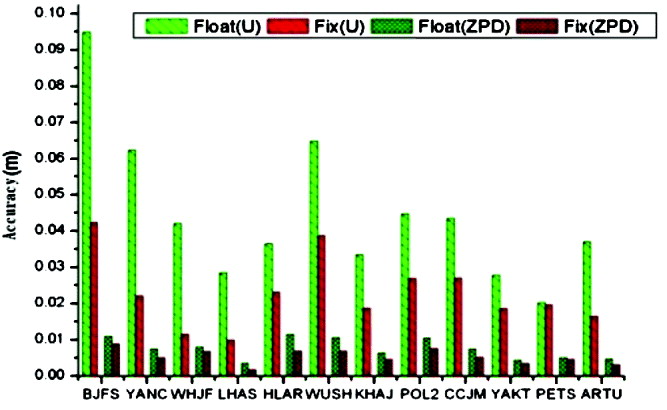
Figure 8. Height and ZPD accuracy of Experiment A.
When examining Figure 7 and Figure 8, one can see that, with thirty minutes of static data, the positioning accuracy of the float solution is 1∼3 cm in the North component, 3∼8 cm in East component and 3∼10 cm in vertical, while the positioning accuracy of the fixed solution is improved to the millimetre level (usually within 5 mm) horizontally and about 1∼4 cm vertically. Moreover, the improvement by the fixed solution on the east component is much more notable. In Figure 8, it can be found that the ZPD accuracy of the fixed and float solutions are generally within 1 cm, while the fixed solution ZPD was improved by 10–30% when compared with the float solution. Some stations (such as ‘LHAS’ and ‘HLAR’) even improved by 50%. According to statistical results, the fixing success rate for stations away from the network, but within 2000 km, is nearly 100%, while that for user stations away from the network over 2000 km is slightly lower but still above 90%. This shows that the UFO products estimated by ten service stations in China can provide high-accuracy rapid GPS positioning and a meteorology service for PPP users within an area up to about 3000 km of the network.
Based on the same analysing strategy used above, similar statistical analysis was carried out for Experiments B and C. Results are shown in Figures 9 to 12.
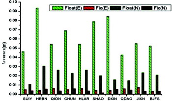
Figure 9. Horizontal accuracy of Experiment B.
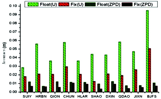
Figure 10. Height and ZPD accuracy of Experiment B.

Figure 11. Horizontal accuracy of Experiment C.

Figure 12. Height and ZPD accuracy of Experiment C.
When examining Figures 9 to 12, similar to those of Experiment A, the positioning accuracy of the fixed solution improved significantly compared to that of the float solution. From Figures 10 and 12, one can find that the ZPD accuracy of both the fixed and float solutions are generally within 1 cm, and the fixed solution ZPD improves by 10–50% compared to the float solution. According to our definition of fixing success rate, the success rates for most stations in the network are close to 100%; the stations away from the network but within 2500 km usually have a success rate of above 90%. The fixing success rate of stations over 3000 km away from the network is still above 80%. This is probably because the user station is too far away from the service network and hence some satellites that are observable from the user station cannot be observed at the tracking stations. Experiment B demonstrates that sparsely distributed IGS tracking stations positioned outside China, with an average spacing of about 2500 km, are already sufficient for reliable, high-accuracy, and rapid positioning as well as meteorological services for the whole country. Experiment C illustrates that UFOs derived from a regional network such as the Chengdu CORS network can also provide reliable and high-accuracy service for PPP users almost countrywide.
5.3. Kinematic Experiment
The GPS data collected on 12 May 2008 (around the Mw 8·0 Wenchuan earthquake in Sichuan Province, China) was selected for the task of retrieving the surface deformation induced by the earthquake. The observations at stations ‘BANA’ and ‘HECU’, which are about 350 km away from the epicentre, were processed in kinematic mode. The results derived from the observations from thirty minutes before to thirty minutes after the earthquake are presented in Figure 13 and Figure 14. The figures on the left show the displacement time series of the float solution while figures on the right show the fixed PPP solution. In the figures, the letters N, E and U denote the north, east and up components respectively. Other stations produced similar results to these two.

Figure 13. Displacement time series of BANA with float solution (a) and fixed solution (b).

Figure 14. Displacement time series of HECU with float solution (a) and fixed solution (b).
As we can see from Figure 13(a) and Figure 14(a), displacements derived from the float solution are comparatively stable in the North direction with an accuracy better than 2 cm, but there are larger fluctuations in the East and vertical components with accuracies of about 5 cm and 10 cm respectively. Therefore, due to the large fluctuations of positioning results, it is not easy to extract the seismic displacement signal since it is easily hidden by noise. It can be seen from Figure 13(b) and Figure 14(b) that the displacement time series of the fixed solution is more stable in the North and East directions with an accuracy of approximately 1∼2 cm, and 5 cm in the vertical direction. The improvement in positioning accuracy by fixing the integer ambiguity shows that PPP can be a promising tool for co-seismic surface displacement monitoring.
6. CONCLUSIONS
We have developed a new approach for estimating Uncalibrated Fractional Offsets (UFOs) using the float estimates of Zero-Differenced (ZD) ambiguities of a reference network as observations. The ZD UFOs of receivers and satellites are estimated in an integrated adjustment which can yield the possibility of fixing integer ZD ambiguities. The estimation and fixing of ambiguities are carried out iteratively, so that the derived ZD UFOs can be of high quality. The approach can be applied to both Wide-Lane (WL) and Narrow-Lane (NL) ambiguities for the estimation of the corresponding UFOs.
The float ZD ambiguities used in this approach can be from network or Precise Point Positioning (PPP) solutions. As the network solution is very time-consuming, the number of stations involved has to be limited, especially for real-time applications. Using the PPP solution, UFOs can be estimated flexibly from a rather dense network. A data processing procedure for providing a PPP service with Integer Ambiguity Resolution has been designed and developed for validating the new approach.
The new approach and the data processing procedure have been validated with several experimental data sets. The UFOs were estimated from reference networks of various scales and provided to users in different locations. From the results, we can conclude that UFOs estimated from the new approach are accurate and reliable enough for achieving PPP with Integer Ambiguity Resolution at a single station on the ZD level. The position and ZPD estimates are significantly improved. The accuracy of static float solutions are generally several centimetres to 10 cm using thirty minutes of observations, while the accuracy of fixed solutions is about 5 mm horizontally and about 2 cm in height. Improvement in the East direction is especially significant. ZPD accuracy obtained in the fixed solution is also improved by 10–50%. The kinematic positioning experiment also demonstrates that a fixed solution can improve PPP accuracy significantly.
The proposed approach is also suitable for providing real-time precise positioning services.
ACKNOWLEDGEMENTS
The authors would like to thank Dr. Maorong Ge from the GeoForschungsZentrum German Research Centre for Geosciences, Potsdam. His advice and guidance were quite valuable and helpful during this research. Thanks also go to the IGS for the GPS data and products.


