


1. Introduction
Since the beginning of the 21st century, life annuity providers have faced an upsurge of pensioners to provide for and the need for reliable, long-term mortality projections is perhaps greater than ever. Indeed, the world-wide increases in life expectancy show no signs of slowing down, and populations where mortality rates are already low still experience rates of improvements of the same, or even higher, magnitude than historically. The situation accentuates the importance of powerful predictive models to handle the consequences of an ever older population.
From a practical point of view, there are two partly conflicting aims: (1) producing accurate forecasts and (2) producing forecasts stable under (annual) updates. Accurate forecasting has been the long-standing objective in actuarial and demographic literature and is, broadly speaking, the goal of the academic, while stability is a more recent requirement pertaining to the needs of the practitioner. When applied in practice, the prevailing market value accounting regime dictates that a mortality model should be updated annually to reflect the latest trends in the data. However, many mortality modelling paradigms are very sensitive to the data period used for calibration, and forecasts can therefore vary substantially from year to year. For an annuity provider, large fluctuations or systematic underperformance of a mortality model can lead to significant shifts in liabilities and capital requirements, resulting in huge costs for either the company or the risk collective. Moreover, throughout Europe, mortality models have become an integral part of policy-making as statutory retirement ages are directly linked to gains in life expectancy. For these decisions, stable short-, medium- and long-term forecasts are not just a requirement, but a necessity.
Stability requirements are particularly difficult to meet when forecasting concerns small populations, including, in fact, many countries. Because improvement patterns in these populations exhibit a great deal of variability, simple extrapolations of past trends tend to have poor predictive power over long horizons and projections are prone to dramatic changes following data updates. This holds true for many of the popular projection methodologies such as the model of Lee and Carter (Reference Lee and Carter1992). In view of these accuracy and stability concerns, Jarner and Kryger (Reference Jarner and Kryger2011) developed the SAINT model that has been used by the Danish, nationwide pension fund ATP, since 2008.
The SAINT model was designed with the purpose of producing stable, biologically plausible long-term projections for adult mortality. More precisely, projections with smooth, increasing age-profiles and gradually changing rates of improvement over time. With the main application of pricing and reserving for long-term pension liabilities in mind, capturing long-term trends reliably were deemed more important than, for example, short-term fit. However, more than a decade’s worth of experience with the SAINT model in use has broadened our understanding of model requirements from the practitioner’s point of view. Even though the overarching structure of the SAINT model has not changed, its components have been revised over the years to address not only accuracy and stability concerns but also the model’s flexibility, explainability and credibility. In this paper, we describe how the SAINT model has evolved since Jarner and Kryger (Reference Jarner and Kryger2011) in response to changing demands arising from practical use and user feedback.
In the years following the introduction of the first version of the SAINT model, quantification of longevity risk became a regulatory requirement. As the deterministic trend component used in Jarner and Kryger (Reference Jarner and Kryger2011) was not able to adequately assess this risk, a version of the SAINT model with a stochastic trend was developed. Eventually, this work led to a generally applicable class of stochastic frailty models, which we present in this paper. This methodology constitutes the main theoretical contribution of the paper.
The rest of the paper is organized as follows. Section 2 contains a survey of the evolution of the SAINT model over the last decade. In Section 3 we discuss how changing rates of improvements can be modelled using frailty. Section 4 formalizes the notion of a stochastic frailty model and develops estimation and forecasting procedures. This is followed by Section 5 presenting a comprehensive application of the SAINT model to international and Danish data. The findings are discussed in light of comparable results from the Lee-Carter model. Finally, Section 6 offers some concluding remarks.
2. The evolution of the SAINT model
ATP is a funded supplement to the Danish state pension, guaranteeing most of the population a whole-life annuity. In 2008, ATP introduced a new market value (whole-life) annuity. The main characteristic of this annuity is that contributions are converted to pension entitlements on a tariff based on prevailing market rates and an annually updated, best estimate, cohort-specific mortality forecast. Once acquired, pension entitlements are guaranteed for life. The structure gives a high degree of certainty for the members, but it leaves ATP with a substantial longevity risk.
The SAINT model was developed as part of the market value annuity, with the specific aim of producing accurate and stable forecasts in order to manage the longevity risk of ATP. Clearly, accuracy is desirable to avoid long-run deficits due to life expectancy increasing faster than expected (or, in the case of life expectancy increasing slower than expected, pension entitlements being too small). However, stability of forecasts is of equal importance. Each update of the model causes a change in the size of technical provisions, which in turn affects the risk capital allocated to cover longevity risk. Effectively, a stable mortality model is “cheaper” than a volatile model, because the former frees up risk capital to be used more efficiently elsewhere, for example, to cover a higher market exposure.
Over the course of the last decade, the SAINT model has undergone a number of changes due to changing demands and feedback from its users. Below, we give a brief presentation of the original SAINT model, followed by a survey of the subsequent major changes and their rationale.
2.1. The original SAINT model
The original SAINT model, as described in Jarner and Kryger (Reference Jarner and Kryger2011), has two core model components:
-
• A reference population consisting of a large, pooled, international data set, and;
-
• A frailty model for modelling increasing rates of improvements over time.
The rationale for using a reference population, in addition to the target population, is that it is easier to extract a long-term trend from a large dataset, than a small dataset, since idiosyncratic features are typically more pronounced in the latter. The mortality of the target population is subsequently linked to the long-term trend. A similar idea, although differently implemented, was introduced by Li and Lee (Reference Li and Lee2005) in their multi-population extension of the Lee-Carter model. Since Jarner and Kryger (Reference Jarner and Kryger2011), the concept of a reference population has appeared in a number of models and applications, for example Cairns et al. (Reference Cairns, Blake, Dowd, Coughlan and Khalaf-Allah2011), Dowd et al. (Reference Dowd, Cairns, Blake, Coughlan and Khalaf-Allah2011), Börger et al. (Reference Börger, Fleischer and Kuksin2014), Villegas and Haberman (Reference Villegas and Haberman2014), Wan and Bertschi (Reference Wan and Bertschi2015), Hunt and Blake (Reference Hunt and Blake2017b), Villegas et al. (Reference Villegas, Haberman, Kaishev and Millossovich2017), Menzietti et al., Reference Menzietti, Morabito and Stranges2019), Li and Liu (Reference Li and Liu2019), Li et al. (Reference Li, Li, Tan and Tickle2019).
In the notation of the present paper, the SAINT model is of the form:
 \begin{align} \mu_{\text{target}}(t,x) &= \mu_{\text{ref}}(t,x)\exp\left(y_t^\top r_x\right), \end{align}
 \begin{align} \mu_{\text{ref}}(t,x) &= \mathbb{E}[Z|t,x]\mu_0(t,x) + \mu_b(t), \end{align}
where
 $\mu_{\text{target}}(t,x)$
and
$\mu_{\text{target}}(t,x)$
and
 $\mu_{\text{ref}}(t,x)$
are the force of mortality at age x and time t of the target and reference population, respectively. The target mortality is linked to the reference mortality by a set of age-dependent regressors,
$\mu_{\text{ref}}(t,x)$
are the force of mortality at age x and time t of the target and reference population, respectively. The target mortality is linked to the reference mortality by a set of age-dependent regressors,
 $r_x$
, with time-dependent coefficients,
$r_x$
, with time-dependent coefficients,
 $y_t$
, termed spread parameters. Further, the reference mortality is modelled by the sum of a multiplicative frailty model with baseline mortality
$y_t$
, termed spread parameters. Further, the reference mortality is modelled by the sum of a multiplicative frailty model with baseline mortality
 $\mu_0$
, and age-independent background mortality,
$\mu_0$
, and age-independent background mortality,
 $\mu_b$
. The term
$\mu_b$
. The term
 $\mathbb{E}[Z|t,x]$
denotes the (conditional) mean frailty of the given cohort, and we will discuss this in detail later. All mortality rates are gender-specific, although this is not shown explicitly in the notation.
$\mathbb{E}[Z|t,x]$
denotes the (conditional) mean frailty of the given cohort, and we will discuss this in detail later. All mortality rates are gender-specific, although this is not shown explicitly in the notation.
Formally, the SAINT model in use today is still of form (2.1)–(2.2), but with a different interpretation of the frailty term, and different specifications of time-series dynamics, regressors, and baseline and background mortality. From a methodological point of view, the new frailty model represents by far the greatest of these changes.
2.2. From deterministic to stochastic frailty
The SAINT model uses frailty to forecast increasing rates of improvement in age-specific mortality, thereby reducing the risk of underestimating future life expectancy gains. Loosely speaking, changes in baseline mortality affect selection and thereby mean frailty,
 $\mathbb{E}[Z|t,x]$
, which in turn modifies the way baseline mortality affect population-level mortality.
$\mathbb{E}[Z|t,x]$
, which in turn modifies the way baseline mortality affect population-level mortality.
In the original SAINT model,
 $\mu_0$
and
$\mu_0$
and
 $\mu_b$
were assumed to be of a form equivalent to
$\mu_b$
were assumed to be of a form equivalent to
 \begin{align} \mu_0(t,x) = \exp\left(\theta_1 + \theta_2 t + \theta_3x + \theta_4 tx + \theta_5 x^2\right), \quad \mu_b(t) = \exp\left(\theta_6 + \theta_7 t\right).\end{align}
This allowed an explicit calculation of
 $\mathbb{E}[Z|t,x]$
and thereby of
$\mathbb{E}[Z|t,x]$
and thereby of
 $\mu_{\text{ref}}$
, assuming gamma-distributed frailties, see (14)–(18) in Jarner and Kryger (Reference Jarner and Kryger2011) for details. The resulting model for
$\mu_{\text{ref}}$
, assuming gamma-distributed frailties, see (14)–(18) in Jarner and Kryger (Reference Jarner and Kryger2011) for details. The resulting model for
 $\mu_{\text{ref}}$
had 8 parameters (
$\mu_{\text{ref}}$
had 8 parameters (
 $\theta_1 - \theta_7$
and a frailty parameter) for each sex, which were estimated by maximizing a standard Poisson likelihood. When forecasting, the parametric form was used to extrapolate
$\theta_1 - \theta_7$
and a frailty parameter) for each sex, which were estimated by maximizing a standard Poisson likelihood. When forecasting, the parametric form was used to extrapolate
 $\mu_{\text{ref}}$
to form a deterministic trend around which
$\mu_{\text{ref}}$
to form a deterministic trend around which
 $\mu_{\text{target}}$
would vary. We refer to this as a deterministic frailty model.
$\mu_{\text{target}}$
would vary. We refer to this as a deterministic frailty model.
Despite its parsimonious structure, the estimated
 $\mu_{\text{ref}}$
-surface provided a remarkable fit to the international dataset. However, it soon became clear that the model was not able to fit other datasets equally well. More importantly, assessment of longevity risk was becoming a regulatory requirement, and for this purpose, a deterministic trend model was insufficient.
$\mu_{\text{ref}}$
-surface provided a remarkable fit to the international dataset. However, it soon became clear that the model was not able to fit other datasets equally well. More importantly, assessment of longevity risk was becoming a regulatory requirement, and for this purpose, a deterministic trend model was insufficient.
The current version of the SAINT model features a stochastic frailty model, in which
 $\mu_0$
and
$\mu_0$
and
 $\mu_b$
are stochastic processes. This implies that the frailty term,
$\mu_b$
are stochastic processes. This implies that the frailty term,
 $\mathbb{E}[Z|t,x]$
, also becomes stochastic, and explicit expressions are no longer available. In order to disentangle the dependence between
$\mathbb{E}[Z|t,x]$
, also becomes stochastic, and explicit expressions are no longer available. In order to disentangle the dependence between
 $\mu_0$
and
$\mu_0$
and
 $\mathbb{E}[Z|t,x],$
a pseudo-likelihood approach, reinterpreting the frailty term in terms of observable quantities, had to be devised. This, in turn, led to a generally applicable “fragilization” method by which essentially any frailty distribution can be combined with any baseline and background mortality to form a model, cf. Section 4.
$\mathbb{E}[Z|t,x],$
a pseudo-likelihood approach, reinterpreting the frailty term in terms of observable quantities, had to be devised. This, in turn, led to a generally applicable “fragilization” method by which essentially any frailty distribution can be combined with any baseline and background mortality to form a model, cf. Section 4.
2.3. Cointegrating gender dynamics
In the original SAINT model, male and female mortality were modelled separately, which resulted in a sex differential of just over 10 years in forecasted cohort life expectancies at birth. When the first version of the stochastic frailty model was implemented, it was therefore decided to model the new stochastic processes via cointegration to ensure better aligned forecasts. At the time, the baseline and background mortality were modelled as
 \begin{align} \mu_0(t,x) = \exp\left(\alpha_t + \beta_t x + 2x^2/10^{4}\right), \quad \mu_b(t) = \exp(\zeta_t),\end{align}
with the processes
 $\{\alpha_t, \beta_t\}$
governing
$\{\alpha_t, \beta_t\}$
governing
 $\mu_0$
being modelled as in Equation (5.5), but with an unrestricted A-matrix. Cointegration reduced the life expectancy difference at birth to about 5 years, and subsequent model development brought it further down to 3.6 years.
$\mu_0$
being modelled as in Equation (5.5), but with an unrestricted A-matrix. Cointegration reduced the life expectancy difference at birth to about 5 years, and subsequent model development brought it further down to 3.6 years.
In Equation (5.5), the B-matrix controls the cointegrating relations, while the A-matrix controls the adjustments to these over time. It later became apparent that an unrestricted A-matrix could lead to complex transitory effects when reestablishing equilibrium relations, as seen on the dashed lines in Figure 1. The resulting projections were hard to justify and communicate, and eventually structural zeros were introduced in A to generate more linear projections. Allowing only pairwise dependence between parameters also offered a greater degree of explainability as the forecasting distribution simplified.

Figure 1. Age 60 actual (dots) and forecasted (lines) period life expectancy using the SAINT model with and without restrictions on the A-matrix from Equation (5.5).
The cointegrating relations and the restrictions placed on the A-matrix were imposed, rather than formally tested. Even though formal testing could be done using the comprehensive statistical framework developed by Johansen (Reference Johansen1995), it was deemed problematic that the underlying time dynamics could change annually following data updates as this would destabilize projections and potentially damage the model’s credibility. Cointegration is therefore used merely as a modelling tool to achieve reasonable projections, rather than to gain insights into the joint behaviour of the time-varying mortality indices, see also Jarner and Jallbjørn (Reference Jarner and Jallbjørn2020) for further discussion on this point.
2.4. Improving the fit
The specification of
 $\mu_0$
in (2.4) was the result of an extensive model search among “simple” models. At the time, it provided a reasonable fit, but eventually failed to adequately capture old-age mortality. Generalizations of linear mortality models typically involve adding a quadratic term to the age effect or introducing cohort components, see for example Cairns et al. (Reference Cairns, Blake, Dowd, Coughlan, Epstein, Ong and Balevich2009). The natural candidate to replace (2.4) was therefore the log-quadratic model
$\mu_0$
in (2.4) was the result of an extensive model search among “simple” models. At the time, it provided a reasonable fit, but eventually failed to adequately capture old-age mortality. Generalizations of linear mortality models typically involve adding a quadratic term to the age effect or introducing cohort components, see for example Cairns et al. (Reference Cairns, Blake, Dowd, Coughlan, Epstein, Ong and Balevich2009). The natural candidate to replace (2.4) was therefore the log-quadratic model
 $\mu_0(t,x) = \exp(\alpha_t + \beta_t x+ \kappa_t x^2)$
. But despite a clearly superior fit, its parameter estimates turned out exceedingly difficult to forecast.
$\mu_0(t,x) = \exp(\alpha_t + \beta_t x+ \kappa_t x^2)$
. But despite a clearly superior fit, its parameter estimates turned out exceedingly difficult to forecast.
After further research into the shape of the mortality age profile, the lack of fit was found to be caused by an inflexibility of (2.4) at the younger ages, a typical problem when fitting parsimonious models over a large age span. By replacing the fixed quadratic term in (2.4) with an excess slope parameter, the low mortality rates of the young were prevented from influencing the trend of the old. The baseline model therefore became
 \begin{equation} \mu_0(t,x) = \exp\left(\widetilde{\alpha}_t+\widetilde{\beta}_t x + \widetilde{\kappa}_t (x-75) \unicode{x1D7D9}_{\{x \geq 75\}}\right).\end{equation}
The model’s parameters are linearized for forecasting purposes through reparametrization, achieved by setting
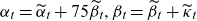 $\alpha_t = \widetilde{\alpha}_t + 75 \widetilde{\beta}_t, \beta_t = \widetilde{\beta}_t + \widetilde{\kappa}_t$
, and
$\alpha_t = \widetilde{\alpha}_t + 75 \widetilde{\beta}_t, \beta_t = \widetilde{\beta}_t + \widetilde{\kappa}_t$
, and
 $\kappa_t = -\widetilde{\kappa}_t$
whereby
$\kappa_t = -\widetilde{\kappa}_t$
whereby
 \begin{equation} \mu_0(t,x) = \exp\left( \alpha_t + \beta_t (x-75) + \kappa_t (x-75) \unicode{x1D7D9}_{\{x < 75\}} \right).\end{equation}
Figure 2 shows the clear improvement in the model’s fit. The fit is particularly impressive at the higher ages and also matches the logistic type behaviour seen in the data for the oldest-old as the frailty component comes into play.

Figure 2. Observed (dots) female death rates for select ages with SAINT fits (solid lines) superimposed. The left panel shows the previous version of SAINT with
 $\mu_0$
as in (2.4), estimated on a dataset with the US included and the window of calibration starting in 1950. The right panel shows the current version of SAINT with
$\mu_0$
as in (2.4), estimated on a dataset with the US included and the window of calibration starting in 1950. The right panel shows the current version of SAINT with
 $\mu_0$
as in (2.5), estimated on a dataset with the US excluded and the window of calibration starting in 1970.
$\mu_0$
as in (2.5), estimated on a dataset with the US excluded and the window of calibration starting in 1970.
2.4.1. Revisiting the reference population and data window
In the original paper, Jarner and Kryger (Reference Jarner and Kryger2011) used an aggregate of international data over the years 1933–2005, including, notably, data from the US. Following the first version of the stochastic frailty model, the left cut point of the data window was updated to 1950, while the right cut point was updated annually to match the most recent available data.
Over the years, it became apparent that the slowdown of the improvement rates in the US had begun to manifest itself in the long-term trend. At the time, the US constituted more than 40% of the reference population. In response, an extensive review of the demographic transitions in the Western world was conducted country for country. This work led to a new paradigm for putting together a more homogeneous and balanced data pool, necessitating an exclusion of the US. In the new dataset, two mortality regimes emerged, and, accordingly, the left cut point of the data window was updated to 1970. We note that other countries have also shown recent stagnating rates of improvement, for example the UK, but overall there has been a continued improvement throughout the period, see Figure 3.

Figure 3. Age 60 actual (dots) and forecasted (lines) period life expectancy using a Lee-Carter model based on a rolling estimation window.
3. Modelling changing rates of improvements
The mortality experience of several countries has shown increasing rates of improvements for older age groups while rates for younger groups have been decelerating, see for example Kannisto et al. (Reference Kannisto, Lauritsen, Thatcher and Vaupel1994), Lee and Miller (Reference Lee and Miller2001), Booth et al. (Reference Booth, Maindonald and Smith2002), Bongaarts (Reference Bongaarts2005), Li et al. (Reference Li, Lee and Gerland2013), Vékás (Reference Vékás2019). For long-term projections, in particular, it is important to model these changes to reduce the risk of underestimating future life expectancy gains.
3.1. Motivating example
Although a plethora of models for modelling and forecasting mortality have been proposed in recent years, see for example Booth (Reference Booth2008) and Janssen (Reference Janssen2018) for an overview, the model of Lee and Carter (Reference Lee and Carter1992) is still by far the most widely used. Lee and Carter (Reference Lee and Carter1992) model the (observed) death rate, m, at time t for age x in a log-bilinear fashion
 \begin{align} \log m(t,x) = a_x + b_x k_t + \varepsilon_{t,x},\end{align}
where a and b are age-specific parameters and k is a time-varying index in which all temporal trends leading to improvements in mortality are encapsulated. The k-index is typically modelled as a random walk with drift, extrapolating the index linearly from the first to the last data point, resulting in constant rates of improvement in forecasted age-specific mortality.
Figure 3 illustrates the problem with assuming constant rates of improvements in forecasts. The figure shows actual and Lee-Carter forecasted period remaining life expectancies at age 60 for Western Europe and Denmark. Except for Western European females, the forecasts vary substantially with the estimation period due to changing rates of improvement. Moreover, the forecasts generally underestimate the future gains in life expectancy because rates of improvement for older age groups tend to increase over time.
This phenomenon is not specific to the Lee-Carter model, but pertains to all models with constant rates of improvements. Fitting these models to shorter, more recent periods of data alleviates the downward bias to some extent, but it does not address the fundamental issue of changing rates. Coherent, multi-population mortality models, for example the model of Li and Lee (Reference Li and Lee2005), can in principle produce changing rates of improvement while the individual populations “lock on” to common rates of improvement. However, the common rates are typically constant over time. Thus, coherence in itself does not guarantee the type of ongoing change in improvement rates that we advocate. For a more detailed discussion of coherent models and their pros and cons, see Jarner and Jallbjørn (Reference Jarner and Jallbjørn2020) and the references therein.
3.2. Frailty theory
Frailty theory rests on the assumption that cohorts are heterogeneous and that some people are more susceptible to death (frail) than others. The difference in frailty causes selection effects in the population and leads to old cohorts being dominated by low mortality individuals.
Frailty theory is well-established in biostatistics and survival analysis, and several monographs are devoted to the topic, for example Duchateau and Janssen (Reference Duchateau and Janssen2008), Wienke (Reference Wienke2010), Hougaard (Reference Hougaard2012). In demographic and actuarial science, frailty models are also known as heterogeneity models. They have been used in mortality modelling to fit the logistic form of old-age mortality, see for example Wang and Brown (Reference Wang and Brown1998), Thatcher (Reference Thatcher1999), Butt and Haberman (Reference Butt and Haberman2004), Olivieri (2006), Cairns et al. (Reference Cairns, Blake and Dowd2006), Spreeuw et al. (Reference Spreeuw, Nielsen and Jarner2013), Li and Liu (Reference Li and Liu2019), and to allow for overdispersion in mortality data, cf. Li et al. (Reference Li, Hardy and Tan2009). The SAINT model, however, employs frailty theory with the dual purpose of fitting old-age mortality and generating changing rates of improvement.
Below, we present a flexible class of continuous time models spanning multiple birth cohorts, with additive frailty and non-frailty components. With additive models, we can distinguish between “selective” mortality influenced by frailty and “background” mortality not affected by frailty, for example accidents. Following Vaupel et al. (Reference Vaupel, Manton and Stallard1979), individual frailty is a non-negative stochastic quantity Z that acts multiplicatively on an underlying baseline mortality rate. We assume that frailty is assigned at birth (according to some distribution) and remains constant throughout an individual’s life span. In this context, we can interpret frailty as individual (congenital) genetic differences. Conditionally on frailty being Z, mortality at age x at time t takes the form
 \begin{align} \mu(t, x | Z ) = Z \mu_0(t,x) + \mu_b(t,x),\end{align}
where
 $\mu_0$
is the baseline rate describing age-period effects influenced by individual frailty and
$\mu_0$
is the baseline rate describing age-period effects influenced by individual frailty and
 $\mu_b$
is background mortality common to all individuals regardless of their respective frailties.
$\mu_b$
is background mortality common to all individuals regardless of their respective frailties.
Equation (3.2) describes the mortality rate of an individual, but this quantity is not observable in population-level data. In fact, we only observe an aggregate of the death rates. We can derive an explicit expression for this aggregate, namely the population-level rate, by writing up the survival function
 \begin{equation}S(t,x) = e^{-\int_0^x \mu(t-x+u,u) \mathop{}\!\textrm{d}{u}} = \mathbb{E}\left[e^{-\int_0^x \mu(t-x+u,u|Z) \mathop{}\!\textrm{d}{u}}\right]\end{equation}
and differentiating
 $- \log S(t,x)$
to get
$- \log S(t,x)$
to get
 \begin{align} \mu(t,x) = \mathbb{E} [Z | t,x] \mu_0(t,x) + \mu_b(t,x).\end{align}
Here,
 $\mathbb{E} [Z|t,x]$
is the mean frailty among the survivors of the cohort born at time
$\mathbb{E} [Z|t,x]$
is the mean frailty among the survivors of the cohort born at time
 $t-x$
. As a matter of convention, we assume without loss of generality that mean frailty is one at birth. It is useful to introduce the Laplace transform
$t-x$
. As a matter of convention, we assume without loss of generality that mean frailty is one at birth. It is useful to introduce the Laplace transform
 $\mathcal{L}(s) = \mathbb{E}[\exp({-}sZ)]$
of the common frailty distribution in which case
$\mathcal{L}(s) = \mathbb{E}[\exp({-}sZ)]$
of the common frailty distribution in which case
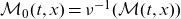
 \begin{equation} \mathbb{E}[Z | t,x] = \frac{-\mathcal{L}'(\mathcal{M}_0(t,x))}{\mathcal{L}(\mathcal{M}_0(t,x))},\end{equation}
where
 $\mathcal{M}_0(t,x) = \int_0^x \mu_0(t-x+u,u) \mathop{}\!\textrm{d}{u}$
is the cumulated baseline rate.
$\mathcal{M}_0(t,x) = \int_0^x \mu_0(t-x+u,u) \mathop{}\!\textrm{d}{u}$
is the cumulated baseline rate.
So far, the expressions above relating mean frailty to the baseline rate are standard in survival analysis. For later use, we establish an additional relationship between mean frailty and the cumulated cohort rate adjusted for background mortality, namely
 \begin{equation} \mathcal{M}(t,x) = \int_0^x \left( \mu(t-x+u,u) - \mu_b(t-x+u,u) \right) \mathop{}\!\textrm{d}{u},\end{equation}
via its survival function
 \begin{equation} \exp({-}\mathcal{M}(t,x)) = S(t,x)e^{\int_0^x \mu_b(t-x+u,u) \mathop{}\!\textrm{d}{u}} = \mathcal{L}(\mathcal{M}_0(t,x)).\end{equation}
Introducing the function
 $\nu(\cdot) = - \log \mathcal{L}(\cdot)$
, we have
$\nu(\cdot) = - \log \mathcal{L}(\cdot)$
, we have
 $\mathcal{M}(t,x) = \nu(\mathcal{M}_0(t,x))$
and
$\mathcal{M}(t,x) = \nu(\mathcal{M}_0(t,x))$
and
 $\mathcal{M}_0(t,x) = \nu^{-1}(\mathcal{M}(t,x))$
which gives us
$\mathcal{M}_0(t,x) = \nu^{-1}(\mathcal{M}(t,x))$
which gives us
 \begin{equation} \mathbb{E}[Z | t,x] = \nu' (\mathcal{M}_0(t,x)) = \nu' ( \nu^{-1} (\mathcal{M}(t,x))),\end{equation}
upon insertion into (3.5).
The relation between mean frailty and mortality described by Equation (3.8) will be central to our estimation approach. Whereas
 $\mathcal{M}_0$
is given solely in terms of the baseline rate,
$\mathcal{M}_0$
is given solely in terms of the baseline rate,
 $\mathcal{M}$
can be estimated using empirical death rates. Substituting
$\mathcal{M}$
can be estimated using empirical death rates. Substituting
 $\mathcal{M}$
by such an estimate disentangles the frailty distribution from the baseline rate which greatly simplifies the estimation procedure whenever parametric structures have been imposed on
$\mathcal{M}$
by such an estimate disentangles the frailty distribution from the baseline rate which greatly simplifies the estimation procedure whenever parametric structures have been imposed on
 $\mu_0$
and
$\mu_0$
and
 $\mu_b$
. We return to the specifics in Section 4.
$\mu_b$
. We return to the specifics in Section 4.
To apply frailty theory in practice, we must identify suitable choices of frailty distributions. A brief account of appropriate distributions is given in Appendix A. Essentially, useful distributions are the ones with an explicit Laplace transform. The most commonly used distribution is the Gamma distribution which has a tractable Laplace transform, see Example 4.1, along with other desirable properties.
3.3. Frailty leads to changing rates of improvements
To clarify how the inclusion of frailty leads to changing rates of improvements, we define the rate of improvement in selective mortality as
 \begin{equation} \rho_s(t,x) = - \frac{\partial}{\partial t} \log \mathbb{E}[Z|t,x] - \frac{\partial}{\partial t} \log \mu_0(t,x),\end{equation}
where
 $\rho_0(t,x) = -\frac{\partial}{\partial t} \log \mu_0(t,x)$
is the rate of improvement in baseline mortality.
$\rho_0(t,x) = -\frac{\partial}{\partial t} \log \mu_0(t,x)$
is the rate of improvement in baseline mortality.
Suppose that we model the period effect so that baseline mortality is decreasing over time, that is,
 $\mu_0(t,x) \rightarrow 0$
as
$\mu_0(t,x) \rightarrow 0$
as
 $t\rightarrow\infty$
for fixed age x. Then, the cumulated baseline will also be decreasing over time, that is
$t\rightarrow\infty$
for fixed age x. Then, the cumulated baseline will also be decreasing over time, that is
 $\mathcal{M}_0(t,x) \rightarrow 0$
as
$\mathcal{M}_0(t,x) \rightarrow 0$
as
 $t \rightarrow \infty$
, while the mean frailty in successive cohorts will be increasing over time due to less and less selection of frail individuals, so
$t \rightarrow \infty$
, while the mean frailty in successive cohorts will be increasing over time due to less and less selection of frail individuals, so
 $\mathbb{E}[Z|t,x] \rightarrow 1$
as
$\mathbb{E}[Z|t,x] \rightarrow 1$
as
 $t \rightarrow \infty$
. From (3.9), we see that improvements in cohort mortality are smaller than, but gradually increasing to, the rate of improvement at the individual level.
$t \rightarrow \infty$
. From (3.9), we see that improvements in cohort mortality are smaller than, but gradually increasing to, the rate of improvement at the individual level.
This line of thinking offers an explanation to the small improvement rates observed in old-age mortality, and it suggests that we might expect to see higher rates of improvements in the future. At old ages where death rates – and thereby selection – are high, the change in mean frailty over time can substantially offset improvements in baseline mortality. This makes improvements in observed mortality close to zero, cf. Equation (3.9), a behaviour illustrated in Figure 4. As improvements in baseline mortality continue to occur at the individual level, the selection mechanism gradually weakens and improvements in observed mortality get closer to the underlying improvement rates. The pattern of gradually changing improvement rates of old-age mortality resembles what is seen in the data. We will return to this point in Section 5.

Figure 4. Illustration of population-level mortality at age 100 over time. When selection is high, observed mortality rates do not improve much even though rates are assumed to be decreasing at the individual level. This is due to improvements in baseline mortality being (partially) offset by increases in mean frailty. As mean frailty eventually approaches one, observed improvements and improvements in the underlying mortality are approximately equal.
3.3.1. The difference between frailty and the traditional cohort perspective
While conditional mean frailty
 $\mathbb{E}[Z|t,x]$
may be regarded as a cohort component in the sense that it focuses on the evolution of a cohort through time, the notion is qualitatively different from the traditional cohort perspective in mortality modelling. As an illustrative example, consider the cohort extended Lee-Carter model of Renshaw and Haberman (Reference Renshaw and Haberman2006), that is
$\mathbb{E}[Z|t,x]$
may be regarded as a cohort component in the sense that it focuses on the evolution of a cohort through time, the notion is qualitatively different from the traditional cohort perspective in mortality modelling. As an illustrative example, consider the cohort extended Lee-Carter model of Renshaw and Haberman (Reference Renshaw and Haberman2006), that is
 \begin{equation} \log \mu(t,x) = a_x+b_xk_t+c_{t-x}.\end{equation}
The cohort component
 $\exp(c_{t-x})$
assumes the role of a dummy variable and offsets mortality by the same factor throughout the life span of individuals born at time
$\exp(c_{t-x})$
assumes the role of a dummy variable and offsets mortality by the same factor throughout the life span of individuals born at time
 $t-x$
. Although the multiple
$t-x$
. Although the multiple
 $\mathbb{E}[Z|t,x] \mu_0(t,x)$
does in principle contain the structure (3.10) with
$\mathbb{E}[Z|t,x] \mu_0(t,x)$
does in principle contain the structure (3.10) with
 $\mu_0(t,x) = \exp(a_x+b_xk_t)$
being the Lee-Carter model,
$\mu_0(t,x) = \exp(a_x+b_xk_t)$
being the Lee-Carter model,
 $\mathbb{E}[Z|t,x]$
is not constant over time except in degenerate cases. Indeed,
$\mathbb{E}[Z|t,x]$
is not constant over time except in degenerate cases. Indeed,
 $\mathbb{E}[Z|t,x]$
progressively decreases for a given cohort as selection intensifies and should therefore not be regarded as a cohort component in the traditional sense.
$\mathbb{E}[Z|t,x]$
progressively decreases for a given cohort as selection intensifies and should therefore not be regarded as a cohort component in the traditional sense.
3.4. Alternative ways of addressing changing improvement rates
With a growing body of empirical evidence against the assumption of constant age-specific rates of improvements, several other approaches have been developed to address the issue. One suggestion involves finding an “optimal” calibration period for which model assumptions are not violated. This usually involves fitting (Lee-Carter) models to shorter and more recent periods of data, see for example Lee and Miller (Reference Lee and Miller2001), Tuljapurkar et al. (Reference Tuljapurkar, Li and Boe2000), Booth et al. (Reference Booth, Maindonald and Smith2002), Li and Li (Reference Li and Li2017). For projections over longer horizons, the problem persists; future increases in especially old-age mortality beyond what has been seen historically cannot be captured by making an informed decision about the period of calibration.
Within the Lee-Carter framework, another solution is to extend the original model by replacing the time-invariant age-response with a time-varying version, so instead of Equation (3.1) we would have
 \begin{equation} \log m(t,x) = a_x + B_{t,x} k_t + \varepsilon_{t,x}.\end{equation}
A freely varying
 $B_{t,x}$
introduces far too many parameters, and some restrictions have to be imposed. Li et al. (Reference Li, Lee and Gerland2013) suggest that
$B_{t,x}$
introduces far too many parameters, and some restrictions have to be imposed. Li et al. (Reference Li, Lee and Gerland2013) suggest that
 $B_{t,x}$
describe the “rotating” pattern of mortality improvements, namely that improvement rates are declining for the young but increasing for the old. Consequently, Equation (3.11) is sometimes referred to as the rotated Lee-Carter model. Li et al. (Reference Li, Lee and Gerland2013) achieve rotation by letting the
$B_{t,x}$
describe the “rotating” pattern of mortality improvements, namely that improvement rates are declining for the young but increasing for the old. Consequently, Equation (3.11) is sometimes referred to as the rotated Lee-Carter model. Li et al. (Reference Li, Lee and Gerland2013) achieve rotation by letting the
 $b_x$
’s from the original model converge (smoothly) to some assumed long-term target
$b_x$
’s from the original model converge (smoothly) to some assumed long-term target
 $B_x$
. The approach has since been adopted and adapted by a number of authors, for example Vékás (Reference Vékás2019) and Gao and Shi (Reference Gao and Shi2021).
$B_x$
. The approach has since been adopted and adapted by a number of authors, for example Vékás (Reference Vékás2019) and Gao and Shi (Reference Gao and Shi2021).
Another idea is to model and project improvement rates directly as opposed to projecting death rates, see for example Haberman and Renshaw (Reference Haberman and Renshaw2012). Various forms of projections built from age-specific improvement rates applied to reference mortality tables are also becoming popular among actuarial practitioners, see for example Jarner and Møller (Reference Jarner and Møller2015) for a detailed account of the longevity benchmark employed by the Danish financial supervisory authority or the model used by the Continuous Mortality Investigation (2016).
The alternative approaches mentioned above each have their own merits as ways of addressing changing rates of improvements. Frailty, however, has the unique advantage that it can be introduced into any existing mortality model to forecast improvement rates higher than those observed historically, while preserving both the original model structure and the underlying driver of the system.
4. Stochastic frailty models
In the following, we detail how frailty can be used with any stochastic mortality model and we show how to estimate and forecast these models. The extension from deterministic to stochastic frailty is a fundamental point in practical applications where the ability to describe uncertainty of forecasts is essential for managing longevity risk.
4.1. Data and terminology
Data are assumed to be on the form of death counts, D(t,x), and corresponding exposures, E(t,x), over time-age cells of the form
 $[t,t+1) \times [x,x+1)$
for a range of calendar years
$[t,t+1) \times [x,x+1)$
for a range of calendar years
 $t\in\{t_{\min}, \dots, t_{\max}\} = \mathcal{T}\subseteq \mathbb N$
and ages
$t\in\{t_{\min}, \dots, t_{\max}\} = \mathcal{T}\subseteq \mathbb N$
and ages
 $x\in\{x_{\min}, \dots, x_{\max}\}=\mathcal{X}\subseteq \mathbb N_0$
. From the death counts and risk exposures, we define the observed (empirical) death rate as the ratio
$x\in\{x_{\min}, \dots, x_{\max}\}=\mathcal{X}\subseteq \mathbb N_0$
. From the death counts and risk exposures, we define the observed (empirical) death rate as the ratio
 \begin{align}m(t,x) = D(t,x)/E(t,x).\end{align}
The empirical death rate is a nonparametric estimate of the underlying cohort rate,
 $\mu(t,x)$
, which for modelling purposes is also assumed constant over
$\mu(t,x)$
, which for modelling purposes is also assumed constant over
 $[t,t+1) \times [x,x+1)$
.
$[t,t+1) \times [x,x+1)$
.
4.2. Modelling framework
For ease of presentation, we will consider stochastic models for baseline and background mortality of the form
 \begin{align} \mu_0(t,x) &= F(\theta_t, \eta_x), \end{align}
 \begin{align} \mu_b(t,x) &= G(\zeta_t, \xi_x), \end{align}
where F and G are functional forms taking parameters in the age-period dimension as input. All quantities may be multidimensional, and further generalizations to include cohort effects and general dependence structures are possible if so desired. We assume that parameters are to be estimated from data, but they can also be fixed or empty.
We define a (generalized) stochastic frailty model as a model of the form
 \begin{align} D(t,x) &\sim \textrm{Poisson}(\mu(t,x) E(t,x)), \end{align}
 \begin{align} \mu(t,x) &= \mathbb{E}[Z|t,x] \mu_0(t,x) + \mu_b(t,x),\end{align}
with
 $\mu_0$
and
$\mu_0$
and
 $\mu_b$
given by (4.2)–(4.3) while
$\mu_b$
given by (4.2)–(4.3) while
 $\mathbb{E}[Z|t,x]$
denotes conditional mean frailty as in Section 3.2. Note that
$\mathbb{E}[Z|t,x]$
denotes conditional mean frailty as in Section 3.2. Note that
 $\mathbb{E}[Z|t,x]$
is now a stochastic quantity since it depends on
$\mathbb{E}[Z|t,x]$
is now a stochastic quantity since it depends on
 $\mu_0$
. The frailty distribution at birth is the same for all cohorts, and it is assumed to belong to a family indexed by
$\mu_0$
. The frailty distribution at birth is the same for all cohorts, and it is assumed to belong to a family indexed by
 $\psi$
with Laplace transform
$\psi$
with Laplace transform
 $\mathcal{L}_\psi$
available in explicit form. The parameters of the model are thus
$\mathcal{L}_\psi$
available in explicit form. The parameters of the model are thus
 $(\psi, \theta, \eta, \zeta, \xi)$
where all components can be vectors.
$(\psi, \theta, \eta, \zeta, \xi)$
where all components can be vectors.
Based on (3.8), we can write
 \begin{align}\mu(t,x) &= \nu^{\prime}_\psi\left(\mathcal{M}_0(t,x)\right) F\left(\theta_t, \eta_x\right) + G\left(\zeta_t, \xi_x\right)\end{align}
with
 $\nu_\psi(\cdot) = - \log \mathcal{L}_\psi(\cdot)$
and
$\nu_\psi(\cdot) = - \log \mathcal{L}_\psi(\cdot)$
and
 $\mathcal{M}_0(t,x) = \sum_{u=0}^{x-1} F(\theta_{u+t-x}, \eta_x)$
. Inserting the above into (4.4), all parameters can be estimated jointly from the resulting likelihood. This likelihood is, however, rather intractable with frailty and remaining parameters occurring in a complex mix. Consequently, estimation has to be handled on a case-by-case basis depending on the choice of frailty distribution and mortality model. Below we propose an alternative, generally applicable pseudo-likelihood approach which greatly simplifies the estimation task.
$\mathcal{M}_0(t,x) = \sum_{u=0}^{x-1} F(\theta_{u+t-x}, \eta_x)$
. Inserting the above into (4.4), all parameters can be estimated jointly from the resulting likelihood. This likelihood is, however, rather intractable with frailty and remaining parameters occurring in a complex mix. Consequently, estimation has to be handled on a case-by-case basis depending on the choice of frailty distribution and mortality model. Below we propose an alternative, generally applicable pseudo-likelihood approach which greatly simplifies the estimation task.
4.3. Pseudo-likelihood function
We seek to replace the problematic term
 $\mathbb{E}[Z|t,x]$
with an estimate that does not depend on baseline parameters. From (3.8), we have that
$\mathbb{E}[Z|t,x]$
with an estimate that does not depend on baseline parameters. From (3.8), we have that
 $\mathbb{E}[Z|t,x] = \nu_\psi'(\nu_\psi^{-1} ( \mathcal{M}(t,x) ))$
, where
$\mathbb{E}[Z|t,x] = \nu_\psi'(\nu_\psi^{-1} ( \mathcal{M}(t,x) ))$
, where
 $\mathcal{M}$
is the cumulated frailty-dependent part of mortality. At first sight, this does not seem to help much since
$\mathcal{M}$
is the cumulated frailty-dependent part of mortality. At first sight, this does not seem to help much since
 $\mathcal{M}$
is even more complicated than
$\mathcal{M}$
is even more complicated than
 $\mathcal{M}_0$
. However, in contrast to
$\mathcal{M}_0$
. However, in contrast to
 $\mathcal{M}_0$
we can obtain an estimate of
$\mathcal{M}_0$
we can obtain an estimate of
 $\mathcal{M}$
which does not involve the baseline parameters. With a slight abuse of notation, suppressing the dependency on the background parameters, we estimate
$\mathcal{M}$
which does not involve the baseline parameters. With a slight abuse of notation, suppressing the dependency on the background parameters, we estimate
 $\mathcal{M}$
by
$\mathcal{M}$
by
 \begin{align} \widetilde{\mathcal{M}}(t,x) = \sum_{u=0}^{x-1} \widetilde{m}(t-x+u,u),\end{align}
where
 \begin{align} \widetilde{m}(t,x) =\begin{cases} m(t_{\min},x) - G(\zeta_{t_{\min}}, \xi_x) & \text{for } x_{\min} \leq x \leq x_{\max} \text{ and } t < t_{\min}, \\[5pt] m(t,x)-G(\zeta_t, \xi_x) & \text{for } x_{\min} \leq x \leq x_{\max} \text{ and } t_{\min} \leq t \leq t_{\max}, \\[5pt] 0 & \text{otherwise}.\end{cases}\end{align}
is an extension of the empirical death rates (with background mortality subtracted). The extension is required because the summation in (4.7) falls partly outside the data window; we need to know the death rates from birth to the present or maximum age for all cohorts entering the estimation. The gray area of Figure 5 illustrates the “missing” death rates. The extension implies that selection prior to
 $t_{\min}$
has happened according to initial rates (rather than actual rates) and that all cohorts have mean frailty one at age
$t_{\min}$
has happened according to initial rates (rather than actual rates) and that all cohorts have mean frailty one at age
 $x_{\min}$
(rather than at birth).
$x_{\min}$
(rather than at birth).

Figure 5. Data are available for years between
 $t_{\min}$
and
$t_{\min}$
and
 $t_{\max}$
and for ages between
$t_{\max}$
and for ages between
 $x_{\min}$
and
$x_{\min}$
and
 $x_{\max}$
. The grey area below and to the left of the data window illustrates the part of the trajectories needed for calculation of
$x_{\max}$
. The grey area below and to the left of the data window illustrates the part of the trajectories needed for calculation of
 $\widetilde{\mathcal{M}}$
that falls outside the data window. The cross-hatched area to the right illustrates the years and ages for which we wish to forecast mortality.
$\widetilde{\mathcal{M}}$
that falls outside the data window. The cross-hatched area to the right illustrates the years and ages for which we wish to forecast mortality.
We propose to base estimation of (4.4)–(4.5) on a likelihood function in which the term
 $\mathbb{E}[Z|t,x]$
is replaced by
$\mathbb{E}[Z|t,x]$
is replaced by
 $\nu_\psi'(\nu_\psi^{-1}( \widetilde{\mathcal{M}}(t,x) ))$
. The resulting approximate likelihood function is referred to as a pseudo-likelihood function, cf. Besag (Reference Besag1975), and corresponds to estimating the modified model
$\nu_\psi'(\nu_\psi^{-1}( \widetilde{\mathcal{M}}(t,x) ))$
. The resulting approximate likelihood function is referred to as a pseudo-likelihood function, cf. Besag (Reference Besag1975), and corresponds to estimating the modified model
 \begin{align} D(t,x) &\sim \textrm{Poisson}(\mu(t,x) E(t,x)), \end{align}
 \begin{align} \mu(t,x) &= \nu^{\prime}_\psi (\nu_\psi^{-1} (\widetilde{\mathcal{M}}(t,x))) F(\theta_t, \eta_x) + G(\zeta_t, \xi_x).\end{align}
Importantly, the cohort rate
 $\mu$
is separable in frailty and baseline parameters. The model is therefore considerably easier to handle than (4.4)–(4.5) in the sense that joint estimation can be based on marginal estimation procedures for the baseline and background intensities,
$\mu$
is separable in frailty and baseline parameters. The model is therefore considerably easier to handle than (4.4)–(4.5) in the sense that joint estimation can be based on marginal estimation procedures for the baseline and background intensities,
 $\mu_0$
and
$\mu_0$
and
 $\mu_b$
. Equation (4.10) might still look daunting, but it simplifies in specific cases.
$\mu_b$
. Equation (4.10) might still look daunting, but it simplifies in specific cases.
Example 4.1 When Z follows a Gamma distribution with mean one and variance
 $\sigma^2,$
the Laplace transform and conditional mean frailty are given by
$\sigma^2,$
the Laplace transform and conditional mean frailty are given by
 \begin{align}\mathcal{L}(s) &= \left( 1 + \sigma^2 s \right)^{-1 / \sigma^2},\qquad\qquad\qquad \end{align}
 \begin{align}\mathbb{E}[Z|t,x] &= \left( 1+ \sigma^2 \mathcal{M}_0(t,x) \right)^{-1} = \exp \left({-}\sigma^2 \mathcal{M}(t,x) \right),\end{align}
whereby Equation (4.10) reads
 \begin{align}\mu(t,x) = \exp\left({-}\sigma^2 \widetilde{\mathcal{M}}(t,x)\right)F(\theta_t, \eta_x) + G(\zeta_t, \xi_x).\end{align}
4.4. Maximum likelihood estimation
Maximum likelihood estimates of the model (4.9)–(4.10) can be obtained by optimizing the profile (pseudo) log-likelihood function,
 \begin{align} \ell(\psi) = \log L\left(\psi, \hat{\theta}(\psi), \hat{\eta}(\psi), \hat{\zeta}(\psi), \hat{\xi}(\psi)\right),\end{align}
where L is the likelihood resulting from (4.9)–(4.10) and
 $\hat{\theta}(\psi), \hat{\eta}(\psi), \hat{\zeta}(\psi)$
and
$\hat{\theta}(\psi), \hat{\eta}(\psi), \hat{\zeta}(\psi)$
and
 $\hat{\xi}(\psi)$
denote the maximum likelihood estimates for fixed value of
$\hat{\xi}(\psi)$
denote the maximum likelihood estimates for fixed value of
 $\psi$
. Since the frailty family is typically of low dimension, the profile log-likelihood function can usually be optimized reliably by general purpose optimization routines. This is particularly simple when
$\psi$
. Since the frailty family is typically of low dimension, the profile log-likelihood function can usually be optimized reliably by general purpose optimization routines. This is particularly simple when
 $\mu_b(t,x) = 0$
for all
$\mu_b(t,x) = 0$
for all
 $t\in\mathcal{T}$
and
$t\in\mathcal{T}$
and
 $x\in\mathcal{X}$
.
$x\in\mathcal{X}$
.
In the general setting with non-zero background mortality, the model describes a situation of competing risks. The interpretation is that individuals of age x at time t are susceptible to death from two different, mutually exclusive sources with intensities
 $\mu_s$
and
$\mu_s$
and
 $\mu_b$
. This structure is natural to consider in many contexts, but the likelihood function is complicated and direct estimation of the parameters may prove difficult even for fixed
$\mu_b$
. This structure is natural to consider in many contexts, but the likelihood function is complicated and direct estimation of the parameters may prove difficult even for fixed
 $\psi$
.
$\psi$
.
Assuming that we have separate routines available for estimating the baseline and background mortality models, we can exploit the additive structure of (4.9)–(4.10) using the EM algorithm of Dempster et al. (Reference Dempster, Laird and Rubin1977). It can be shown that the likelihood is increased in each step of the EM algorithm and thus converges to a local maximum, although it may do so rather slowly. It is, however, a great advantage that we can use the same top-level procedure to estimate virtually any combination of mortality models, especially when estimation routines for the underlying models are readily available. It is also straightforward to extend the EM algorithm to more than two competing risks.
Alternatively, if computational efficiency is essential, we can carry out estimation by Newton-Raphson sweeps over frailty and mortality model parameters, but this requires a substantial amount of tailor-made code. We find that optimizing the log-likelihood using the EM algorithm is both flexible, easy to implement and in our experience sufficiently fast and robust to be of practical use. The algorithm is detailed in Appendix B.
4.5. Forecasting
Suppose that we have estimates
 $(\hat{\psi}, \hat{\theta}, \hat{\eta}, \hat{\zeta}, \hat{\xi})$
available. Following the usual approach in stochastic mortality modelling, death rates are to be projected using a time-series model for the time-varying parameters
$(\hat{\psi}, \hat{\theta}, \hat{\eta}, \hat{\zeta}, \hat{\xi})$
available. Following the usual approach in stochastic mortality modelling, death rates are to be projected using a time-series model for the time-varying parameters
 $\{\theta_t, \zeta_t\}_{t \in \mathcal{T}}$
. Typically, a (multidimensional) random walk with drift is used, see for example Lee and Carter (Reference Lee and Carter1992) or Cairns et al. (Reference Cairns, Blake and Dowd2006), but models with more complex structure can also be applied. Let an overbar denote projected parameters and assume that these are available for
$\{\theta_t, \zeta_t\}_{t \in \mathcal{T}}$
. Typically, a (multidimensional) random walk with drift is used, see for example Lee and Carter (Reference Lee and Carter1992) or Cairns et al. (Reference Cairns, Blake and Dowd2006), but models with more complex structure can also be applied. Let an overbar denote projected parameters and assume that these are available for
 $t \in \{t_{\max}+1, \dots, t_{\max}+h\}$
given a forecasting horizon
$t \in \{t_{\max}+1, \dots, t_{\max}+h\}$
given a forecasting horizon
 $h \in \mathbb N_+$
. The forecast region is illustrated as the cross-hatched box in Figure 5.
$h \in \mathbb N_+$
. The forecast region is illustrated as the cross-hatched box in Figure 5.
Baseline and background mortality rates are readily projected by inserting
 $\bar{\theta}_t$
and
$\bar{\theta}_t$
and
 $\hat{\eta}_x$
into (4.2) and
$\hat{\eta}_x$
into (4.2) and
 $\bar{\zeta}_t$
and
$\bar{\zeta}_t$
and
 $\hat{\xi}_x$
into (4.3). Forecasting mean frailty is slightly more involved. We notice that while it was convenient to specify mean frailty in terms of
$\hat{\xi}_x$
into (4.3). Forecasting mean frailty is slightly more involved. We notice that while it was convenient to specify mean frailty in terms of
 $\mathcal{M}$
for estimation purposes, it is practical to express it in terms of
$\mathcal{M}$
for estimation purposes, it is practical to express it in terms of
 $\mathcal{M}_0$
when forecasting, because
$\mathcal{M}_0$
when forecasting, because
 $\mathcal{M}_0$
can be computed directly from F throughout the forecast region. Mortality is thus projected via
$\mathcal{M}_0$
can be computed directly from F throughout the forecast region. Mortality is thus projected via
 \begin{align} \mu(t,x) = \nu^{\prime}_{\hat{\psi}} \left(\widetilde{\mathcal{M}}_0(t,x)\right) F\left(\bar{\theta}_t, \hat{\eta}_x\right) + G\left(\bar{\zeta}_t, \hat{\xi}_x\right),\end{align}
where
 $\widetilde{\mathcal{M}}_0(t,x)$
in the forecast region is given by the recursion
$\widetilde{\mathcal{M}}_0(t,x)$
in the forecast region is given by the recursion
 \begin{align} \widetilde{\mathcal{M}}_0(t,x) =\begin{cases} \widetilde{\mathcal{M}}_0\left(t_{\max},x-1\right) + F\!\left(\hat{\theta}_{t_{\max}}, \hat{\eta}_{x-1}\right) & \!\!\text{for } x_{\min} < x \text{ and } t_{\max}+1 = t, \\[8pt] \widetilde{\mathcal{M}}_0(t-1, x-1) + F\!\left(\bar{\theta}_{t_{\max}}, \hat{\eta}_{x-1}\right) & \!\!\text{for } x_{\min} < x \text{ and } t_{\max}+1 < t, \\[4pt] 0 & \!\!\text{for } x_{\min} = x.\end{cases}\end{align}
We underline that G does not enter
 $\widetilde{\mathcal{M}}_0$
in the forecast, whereas in the data window
$\widetilde{\mathcal{M}}_0$
in the forecast, whereas in the data window
 $\widetilde{\mathcal{M}}_0$
is defined by the transformation
$\widetilde{\mathcal{M}}_0$
is defined by the transformation
 $\widetilde{\mathcal{M}}_0(t,x) = \nu_{\hat{\psi}}^{-1}(\widetilde{\mathcal{M}}(t,x))$
to ensure consistency with the estimated model.
$\widetilde{\mathcal{M}}_0(t,x) = \nu_{\hat{\psi}}^{-1}(\widetilde{\mathcal{M}}(t,x))$
to ensure consistency with the estimated model.
Example 4.2 Continuing Example 4.1 where frailty is Gamma distributed with mean one and estimated variance
 $\hat{\sigma}^2$
, we get using (4.12) in conjunction with (4.15) that mortality should be forecasted via
$\hat{\sigma}^2$
, we get using (4.12) in conjunction with (4.15) that mortality should be forecasted via
 \begin{align}\mu(t,x) = \left(1+\hat{\sigma}^2\widetilde{\mathcal{M}}_0(t,x)\right)^{-1} F(\bar{\theta}, \hat{\eta}_x) + G(\bar{\zeta}_t, \hat{\xi}_x),\end{align}
with
 $\widetilde{\mathcal{M}_0}$
given by (4.16) in the forecast region. In the data window,
$\widetilde{\mathcal{M}_0}$
given by (4.16) in the forecast region. In the data window,
 $\widetilde{\mathcal{M}}_0(t,x)$
can be expressed as
$\widetilde{\mathcal{M}}_0(t,x)$
can be expressed as
 $\widetilde{\mathcal{M}}_0(t,x) = [\exp(\hat{\sigma}^2 \widetilde{\mathcal{M}}(t,x)) - 1]/\hat{\sigma}^2$
using (4.12).
$\widetilde{\mathcal{M}}_0(t,x) = [\exp(\hat{\sigma}^2 \widetilde{\mathcal{M}}(t,x)) - 1]/\hat{\sigma}^2$
using (4.12).
5. An application to international mortality
We consider the implementation of the stochastic frailty model currently used at ATP and make comparisons to the usual Lee-Carter methodology. The application is based on mortality data retrieved from the Human Mortality Database (2021). To allow the reader to reproduce the results, we use Danish data to model the spread, rather than proprietary ATP data. Sections 5.1–5.3 cover reference population mortality, while Section 5.4 discusses spread modelling for target population mortality.
5.1. An international reference trend
The reference mortality trend, denoted
 $\mu_{\text{ref}}$
, belongs to the class of stochastic frailty models (4.2)–(4.3) and is gender-specific although this is not shown explicitly in the notation. The model assumes Gamma distributed frailty with mean one and variance
$\mu_{\text{ref}}$
, belongs to the class of stochastic frailty models (4.2)–(4.3) and is gender-specific although this is not shown explicitly in the notation. The model assumes Gamma distributed frailty with mean one and variance
 $\sigma^2$
and takes the functional form
$\sigma^2$
and takes the functional form
 \begin{align}\mu_{\text{ref}}(t,x) &= \exp\left({-}\sigma^2 \widetilde{\mathcal{M}}(t,x)\right) \mu_0(t,x) + \mu_b(t),\qquad\quad\ \end{align}
 \begin{align}\mu_0(t,x) &= \exp\left( \alpha_t + \beta_t (x-75) + \kappa_t (x-75) \unicode{x1D7D9}_{\{x < 75\}} \right), \end{align}
 \begin{align}\mu_b(t) &= \exp\left(\zeta_t\right).\qquad\qquad\qquad\qquad\qquad\quad\qquad\end{align}
In (5.1), the variance of the frailty distribution expresses the amount of heterogeneity in the population, but since any estimate depends on the choice of
 $\mu_0$
, the quantity can only be interpreted in a model-specific context. On the other hand, its influence on the mortality curve is clear. If death rates increase with age, the function
$\mu_0$
, the quantity can only be interpreted in a model-specific context. On the other hand, its influence on the mortality curve is clear. If death rates increase with age, the function
 $x \mapsto \exp({-}\sigma^2\widetilde{\mathcal{M}}(t,x))$
decreases from one towards zero and describes how
$x \mapsto \exp({-}\sigma^2\widetilde{\mathcal{M}}(t,x))$
decreases from one towards zero and describes how
 $\mu_0$
is “dragged” down by the frailty component. If
$\mu_0$
is “dragged” down by the frailty component. If
 $\sigma^2$
is close to zero, then mean frailty is close to one for all ages. As the variance grows, the decline in mean frailty steepens. This drags down the old-age part of the mortality curve and eventually so much that the rates fall into a decline.
$\sigma^2$
is close to zero, then mean frailty is close to one for all ages. As the variance grows, the decline in mean frailty steepens. This drags down the old-age part of the mortality curve and eventually so much that the rates fall into a decline.
5.1.1. A Lee-Carter baseline?
Instead of the Gompertzian model applied in (5.2), one could use a Lee-Carter model for
 $\mu_0$
, see Jarner (Reference Jarner2014) for such an application. However, we find that the parametric structure in (5.2) is favourable in terms of stability and preserving the overall structure of the data and, in particular, smooth and increasing age-profiles, which is not guaranteed in long-term Lee-Carter forecasts.
$\mu_0$
, see Jarner (Reference Jarner2014) for such an application. However, we find that the parametric structure in (5.2) is favourable in terms of stability and preserving the overall structure of the data and, in particular, smooth and increasing age-profiles, which is not guaranteed in long-term Lee-Carter forecasts.
Moreover, the parameters of the Lee-Carter model are not identifiable without additional constraints which precludes the use of more flexible time dynamics such as error-correction models, a limitation the parametric (identifiable) structure does not have, see for example Hunt and Blake (Reference Hunt and Blake2017a) and Jarner and Jallbjørn (Reference Jarner and Jallbjørn2020) for a detailed discussion.
Lastly, unlike the parametric form (5.2) that readily expands in the age dimension, that is the model extends to ages not part of the estimation, the Lee-Carter model applies only to the age span used in the calibration. This is a pronounced problem at the highest ages where data are often sparse. To obtain reliable and stable rates in both model and forecasts, one typically employs a Kannisto extension (Kannisto et al., Reference Kannisto, Lauritsen, Thatcher and Vaupel1994), or a similar procedure, for example the methods discussed in Pitacco et al. (Reference Pitacco, Denuit, Haberman and Olivieri2009), for the oldest-old. Irrespective of the extrapolation procedure, the coupling of two separate models adds an additional layer of complexity and defeats part of the purpose for introducing frailty, namely to capture the logistic type old-age mortality behaviour seen in the data.
5.1.2. Selecting a suitable reference population
To establish an international reference population, we have to decide on a suitable list of countries to use. While all countries appear to follow the same long-term trend, mortality improvements occur at different times for individual countries and variation in improvement rates differ as well. Ideally, the reference trend should consist of countries that reflect the prevalent mortality regime, but their historical development ought to be comparable as well. That is, the countries chosen ought to have undergone the same stages of demographic transition at roughly the same time.
It proves quite difficult to find a set of rules for selecting countries satisfying these broad criteria. Kjærgaard et al. (Reference Kjærgaard, Canudas-Romo and Vaupel2016) propose an out-of-sample selection criterion as a way of constructing an “optimal” set of countries. Others have established hard inclusion criteria based on various socio-demographic-indicators, for example the Dutch actuarial society who base their official projections on a peer group of all European countries with a per capita GDP above the European average (Antonio et al. Reference Antonio, Devriendt, Boer, Vries, Waegenaere, Kan, Kromme, Ouburg, Schulteis, Slagter, Winden, Iersel and Vellekoop2017).
We remain agnostic with regard to specific rules. Having populations entering or leaving the data pool following (annual) data updates is almost certainly bound to cause problems in terms of model stability. Our advice is to choose a wide range of countries with the intention of sticking with them in the long term. With an outset in the countries available from the Human Mortality Database and excluding countries only if they clearly violate the criteria above, we are left with primarily the western part of Europe. In particular, the SAINT model is currently based on pooled data from the following 18 countries: Australia, Austria, Belgium, Canada, Denmark, Finland, France, Germany (West), Iceland, Italy, Luxembourg, Netherlands, Norway, Scotland, Spain, Sweden, Switzerland and UK (England and Wales).
5.2. Time dynamics
The SAINT model (5.2)–(5.3) has four time-varying parameters that need to be forecasted (for each sex). The Makeham component
 $\zeta$
and the excess slope
$\zeta$
and the excess slope
 $\kappa$
are nuisance parameters included in the model to add sufficient flexibility to fit the historical data and to enhance interpretability of the level
$\kappa$
are nuisance parameters included in the model to add sufficient flexibility to fit the historical data and to enhance interpretability of the level
 $\alpha$
and the slope
$\alpha$
and the slope
 $\beta$
. Even though
$\beta$
. Even though
 $\{\zeta_t\}_{t\in\mathcal{T}}$
and
$\{\zeta_t\}_{t\in\mathcal{T}}$
and
 $\{\kappa_t\}_{t\in\mathcal{T}}$
appear non-stationary, see Figure 6, modelling their trending behaviour has little effect on mortality projections. Striking a compromise between model complexity and performance, we forecast these parameters using a random walk without drift, so for any horizon
$\{\kappa_t\}_{t\in\mathcal{T}}$
appear non-stationary, see Figure 6, modelling their trending behaviour has little effect on mortality projections. Striking a compromise between model complexity and performance, we forecast these parameters using a random walk without drift, so for any horizon
 $h \in \mathbb{N}_0$
we have
$h \in \mathbb{N}_0$
we have
 \begin{equation}\kappa_{t_{\max}+h}|\kappa_{t_{\max}} \sim \mathcal{N}\left(\kappa_{t_{\max}}, h \sigma_\kappa^2 \right) \quad \text{and} \quad \zeta_{t_{\max}+h}|\zeta_{t_{\max}} \sim \mathcal{N}\left(\zeta_{t_{\max}}, h \sigma_\zeta^2 \right),\end{equation}
where
 $\sigma_\kappa, \sigma_\zeta \in \mathbb R_+$
.
$\sigma_\kappa, \sigma_\zeta \in \mathbb R_+$
.
Projecting
 $\{\alpha_t, \beta_t\}$
is a more delicate task. In particular, some thought should go into the joint behaviour of the gender-specific forecasts. It is a well-established fact that women live longer than men and while this gender gap varies over time it is believed to persist. Since forecasting even closely related populations independently will lead to diverging forecasts, cf. Tuljapurkar et al. (Reference Tuljapurkar, Li and Boe2000), we must deal with the problem through joint modelling in order not to have undesirable scenarios such as projecting men to live longer than women.
$\{\alpha_t, \beta_t\}$
is a more delicate task. In particular, some thought should go into the joint behaviour of the gender-specific forecasts. It is a well-established fact that women live longer than men and while this gender gap varies over time it is believed to persist. Since forecasting even closely related populations independently will lead to diverging forecasts, cf. Tuljapurkar et al. (Reference Tuljapurkar, Li and Boe2000), we must deal with the problem through joint modelling in order not to have undesirable scenarios such as projecting men to live longer than women.
5.2.1. An error-correction model
To ensure that female and male parameters “stay together,” not just in a median forecast but also for every stochastic realization, we need parameters to cointegrate, that is a given linear combination of them should be stationary. This is achieved by forecasting from the error-correction model
 \begin{align} \Delta Y_t = A B^\top Y_{t-1} + C + \omega_t,\end{align}
where
 $\omega_t \stackrel{\textrm{iid}}\sim \mathcal{N}_4(0, \Omega)$
,
$\omega_t \stackrel{\textrm{iid}}\sim \mathcal{N}_4(0, \Omega)$
,
 $\Delta Y_t = Y_t - Y_{t-1}$
and
$\Delta Y_t = Y_t - Y_{t-1}$
and
 \begin{equation} Y_t = \begin{pmatrix} \alpha^f_t \\[4pt] \alpha_t^m \\[4pt] \beta_t^f \\[4pt] \beta_t^m \end{pmatrix}, \quad A = \begin{pmatrix} a_{11} & \quad 0 \\[4pt] a_{21} & \quad 0 \\[4pt] 0 & \quad a_{32} \\[4pt] 0 & \quad a_{42} \end{pmatrix}, \quad B = \begin{pmatrix} \phantom{-}1 & \quad \phantom{-}0 \ \\[4pt] -1 & \quad \phantom{-}0 \ \\[4pt] \phantom{-}0 & \quad \phantom{-}1 \ \\[4pt] \phantom{-}0 & \quad -1 \ \end{pmatrix}, \quad C = \begin{pmatrix} c_1 \\[4pt] c_2 \\[4pt] c_3 \\[4pt] c_4 \end{pmatrix},\end{equation}
with superscript f and m denoting female and male parameter values, respectively. Equation (5.6) contains two critical assumptions:
-
1. Structural zero’s have been placed in the A-matrix making parameter pairs weakly exogenous, so that the relation between the
 $\alpha$
’s will not affect the relation between the
$\beta$
’s and vice versa.
$\alpha$
’s will not affect the relation between the
$\beta$
’s and vice versa. -
2. The B-matrix imposes two cointegrating relations, one between each parameter pair, with coefficients of unity so that the model corrects any disequilibrium that may arise in the difference between the parameters.


The error-correction behaviour of (5.5) can be made more precise by decomposing the drift term. For a
 $p \times q$
matrix X of full rank, we say that another matrix
$p \times q$
matrix X of full rank, we say that another matrix
 $X_\perp$
of full rank and dimension
$X_\perp$
of full rank and dimension
 $p \times (p-q)$
such that
$p \times (p-q)$
such that
 $X^\top X_\perp=0$
is its orthogonal complement. With
$X^\top X_\perp=0$
is its orthogonal complement. With
 $M = A(B^\top A)^{-1} B^\top,$
it can be shown that
$M = A(B^\top A)^{-1} B^\top,$
it can be shown that
 $I-M = B_\perp (A_\perp^\top B_\perp)^{-1} A_\perp^\top$
, cf. Chapter 3 of Johansen (Reference Johansen1995). Using this identity, we can rewrite (5.5) so that
$I-M = B_\perp (A_\perp^\top B_\perp)^{-1} A_\perp^\top$
, cf. Chapter 3 of Johansen (Reference Johansen1995). Using this identity, we can rewrite (5.5) so that
 \begin{equation} \Delta Y_t = A\left(B^\top Y_{t-1} - C_D\right) + C_\Delta + \omega_t,\end{equation}
where
 $C_D = -(B^\top A)^{-1}B^\top C = \left(C_{D_\alpha}, C_{D_\beta} \right)^\top$
is the parameter difference in stationarity with
$C_D = -(B^\top A)^{-1}B^\top C = \left(C_{D_\alpha}, C_{D_\beta} \right)^\top$
is the parameter difference in stationarity with
 $C_{D_\alpha} = \frac{c_1-c_2}{a_{21}-a_{11}}$
and
$C_{D_\alpha} = \frac{c_1-c_2}{a_{21}-a_{11}}$
and
 $C_{D_\beta} = \frac{c_3-c_4}{a_{42}-a_{32}}$
, while
$C_{D_\beta} = \frac{c_3-c_4}{a_{42}-a_{32}}$
, while
 $C_\Delta = (I-M) C = (C_{\Delta_\alpha}, C_{\Delta_\alpha}, C_{\Delta_\beta}, C_{\Delta_\beta})^\top$
is the common drift with
$C_\Delta = (I-M) C = (C_{\Delta_\alpha}, C_{\Delta_\alpha}, C_{\Delta_\beta}, C_{\Delta_\beta})^\top$
is the common drift with
 $C_{\Delta_\alpha} = \frac{a_{21}c_1-a_{11}c_2}{a_{21}-a_{11}}$
and
$C_{\Delta_\alpha} = \frac{a_{21}c_1-a_{11}c_2}{a_{21}-a_{11}}$
and
 $ C_{\Delta_\beta} = \frac{a_{42}c_3-a_{32}c_4}{a_{42}-a_{32}}$
. From Equation (5.7), it is clear
$ C_{\Delta_\beta} = \frac{a_{42}c_3-a_{32}c_4}{a_{42}-a_{32}}$
. From Equation (5.7), it is clear
 $Y_t$
is updated in response to the disequilibrium error
$Y_t$
is updated in response to the disequilibrium error
 $B^\top Y_{t-1}-C_D$
with a force depending on the magnitude of the a’s.
$B^\top Y_{t-1}-C_D$
with a force depending on the magnitude of the a’s.
An explicit representation of the (median) forecast for a horizon
 $h \in \mathbb N_0$
can be discerned via the Granger representation theorem, see for example Jarner and Jallbjørn (Reference Jarner and Jallbjørn2020). We have
$h \in \mathbb N_0$
can be discerned via the Granger representation theorem, see for example Jarner and Jallbjørn (Reference Jarner and Jallbjørn2020). We have
 \begin{align} \mathbb{E} \left[Y_{t_{\max}+h}|Y_{t_{\max}}\right] = & Y_{t_{\max}} + C_\Delta h\nonumber\\[5pt]& - A\left(B^\top A\right)^{-1} \begin{pmatrix} 1-\lambda_\alpha^h & \quad 0 \\[4pt] 0 & \quad 1-\lambda_\beta^h \end{pmatrix} \left(B^\top Y_{t_{\max}} - C_D\right),\end{align}
where
 $\lambda_\alpha = 1 + a_{11} - a_{21}$
and
$\lambda_\alpha = 1 + a_{11} - a_{21}$
and
 $\lambda_\beta = 1 + a_{32} - a_{42}$
are eigenvalues of
$\lambda_\beta = 1 + a_{32} - a_{42}$
are eigenvalues of
 $I + AB^\top$
. Equation (5.8) highlights the asymptotic random walk behaviour, with the initial disequilibrium error decaying exponentially to zero provided that
$I + AB^\top$
. Equation (5.8) highlights the asymptotic random walk behaviour, with the initial disequilibrium error decaying exponentially to zero provided that
 $\lambda_\alpha, \lambda_\beta <1$
.
$\lambda_\alpha, \lambda_\beta <1$
.
Writing out the error-correction behaviour helps us identify means of ensuring stable and robust forecasts. With this aim in mind, adjusting
 $C_D$
and
$C_D$
and
 $C_\Delta$
to equal desired long-term values might be preferable compared to unconstrained estimation. Equation (5.8) details how the target equilibrium may severely affect projections. It shows that the error-correction model can bring about a number of undesirable features in the median forecast, like short- to medium-term increases in mortality for one of the genders during the restoration of the equilibrium. It is difficult to justify such behaviours in best estimate projections. To avoid them, we assume that
$C_\Delta$
to equal desired long-term values might be preferable compared to unconstrained estimation. Equation (5.8) details how the target equilibrium may severely affect projections. It shows that the error-correction model can bring about a number of undesirable features in the median forecast, like short- to medium-term increases in mortality for one of the genders during the restoration of the equilibrium. It is difficult to justify such behaviours in best estimate projections. To avoid them, we assume that
 $B^\top Y_t$
is distributed according to its stationary distribution by equating
$B^\top Y_t$
is distributed according to its stationary distribution by equating
 $C_D$
to the difference between jump-off values, namely
$C_D$
to the difference between jump-off values, namely
 $\widehat{C}_{D_\theta} = \widehat{\theta}^f_{t_{\max}} - \widehat{\theta}^m_{t_{\max}}$
where
$\widehat{C}_{D_\theta} = \widehat{\theta}^f_{t_{\max}} - \widehat{\theta}^m_{t_{\max}}$
where
 $\theta$
is either
$\theta$
is either
 $\alpha$
or
$\alpha$
or
 $\beta$
. This makes the median forecast of the error-correction model coincide with the median forecast of a random walk model, since the ultimate term in (5.8) vanishes. The error-correction interpretation still applies, however, when considering a stochastic realization of the process. Moreover, looking at the evolution of mortality through the years, for example Figure 3, it is clear that female mortality has developed more steadily than mortality for the males. We therefore use the empirical average of the female parameters to model the common slope, that is
$\beta$
. This makes the median forecast of the error-correction model coincide with the median forecast of a random walk model, since the ultimate term in (5.8) vanishes. The error-correction interpretation still applies, however, when considering a stochastic realization of the process. Moreover, looking at the evolution of mortality through the years, for example Figure 3, it is clear that female mortality has developed more steadily than mortality for the males. We therefore use the empirical average of the female parameters to model the common slope, that is
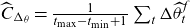 $\widehat{C}_{\Delta_\theta} = \frac{1}{t_{\max}-t_{\min}+1}\sum_t \Delta \widehat{\theta}_{t}^f$
where
$\widehat{C}_{\Delta_\theta} = \frac{1}{t_{\max}-t_{\min}+1}\sum_t \Delta \widehat{\theta}_{t}^f$
where
 $\theta$
is either
$\theta$
is either
 $\alpha$
or
$\alpha$
or
 $\beta$
.
$\beta$
.
5.3. Model fit and forecast
Since international mortality develops more steadily than country-specific mortality, we are able to use a relatively wide window of data for model calibration. The endpoints should be chosen such that we do not introduce structural breaks if data for some countries are missing. Balancing these concerns, we apply the model to international mortality data, ages 20–100 and calendar years 1970–2017 with 2017 being the last year where data exist for all the countries considered at the time of writing. The model is estimated separately for females and males, and follows the EM algorithm described in Appendix B.
The estimated parameters of the SAINT model (5.2)–(5.3) are shown in Figure 6. To justify the use of the error-correction model (5.5), the series
 $\{\alpha_t\}_{t\in\mathcal{T}}$
and
$\{\alpha_t\}_{t\in\mathcal{T}}$
and
 $\{\beta_t\}_{t\in\mathcal{T}}$
must be integrated of order 1 for both genders, that is the stochastic part of these processes must be non-stationary. We conclude from unit root tests (test results not shown) that this is indeed the case. Further, we take the observed stable difference between parameters as (weak) evidence that they engage in an equilibrium correcting relationship.
$\{\beta_t\}_{t\in\mathcal{T}}$
must be integrated of order 1 for both genders, that is the stochastic part of these processes must be non-stationary. We conclude from unit root tests (test results not shown) that this is indeed the case. Further, we take the observed stable difference between parameters as (weak) evidence that they engage in an equilibrium correcting relationship.

In mortality forecasting applications, the choice of jump-off point is a key consideration to match the start of the projection with recently observed data (Lee and Miller Reference Lee and Miller2001). Because the SAINT model fits the empirical death rates very well, cf. Figure 2, no jump-off correction is needed and we use the model values in the jump-off year to determine the jump-off rates. Moreover, the Poisson assumption (4.4) ensures that the model approximates the total number of deaths in the data, see also the discussion in Brouhns et al. (Reference Brouhns, Denuit and Vermunt2002).
5.3.1. Comparing SAINT and Lee-Carter forecasts
To put forecasting into perspective, the SAINT projections are compared to projections generated by a Lee-Carter model. The Lee-Carter model is, in the spirit of this paper, estimated under the Poisson assumption as in Brouhns et al. (Reference Brouhns, Denuit and Vermunt2002), and we use a random walk with drift for forecasting as is customary. Extrapolating the time-varying index linearly implies that age-specific death rates decay exponentially at a constant rate. We shall see that this assumption causes forecasts based on the Lee-Carter methodology to have a tendency of underestimating the actual gains in old-age mortality. The purpose of the comparison is not to show superiority of SAINT over other models, but to illustrate the beneficial effects of cointegration and frailty.
Forecasts are compared by considering period life expectancies. While cohort life expectancies taking future improvements of mortality into account are generally of more interest, the period life expectancy summarizes the level of mortality at a given time and is better suited for illustrative purposes as it can be compared with the actual experience. Recently, Arnold et al. (Reference Arnold, Jijiie, Jondeau and Rockinger2019) added perspective on the stability of period versus cohort tables, arguing that the former might be preferable for practitioners looking to minimize capital adjustments following life tables updates.
Historical and forecasted life expectancies of a 60-year-old are shown in Figure 7. The figure shows that both models produce highly similar median forecasts for female life expectancy and that predictions are quite robust to the choice of the data window used to calibrate the model. This similarity can be attributed to the stable rates of improvements observed since the 1970s. For the males, however, the improvement rates considered during the period of estimation are considerably lower than the actual rates in the periods that follow. The Lee-Carter model fails to capture this development, and the median forecasts are a good way from agreeing with the actual experience. Since improvement rates are increasing over time, predictions from the Lee-Carter model grow increasingly optimistic as we include more recent data.

Figure 7. The panels show actual (dots) and forecasted (lines) remaining life expectancies for age 60 females and males with pointwise 95% confidence bands based on expanding estimation windows. Even though a rolling fixed-length data window is a more common back test approach in the literature, an expanding data window corresponds to how a mortality model is typically updated in practice.
The SAINT model lends its strength in the stable female improvement rates by the coupling of the genders described in Section 5.2. This leads to the forecasts being decidedly more robust to the choice of estimation period, and the resulting almost linear median life expectancy projections resemble the actual experience better than the scattered Lee-Carter forecasts. In fact, it is quite remarkable how well even the first SAINT forecast based on 1970-1989 predicts present day male life expectancy.
To contrast the forecasting uncertainty of the two methods, Table 1 reports summary statistics for the projected life time distributions based on 10,000 simulations. Both the table and the figure reveal that there is a major difference in the forecasting uncertainty between the two methods, even when point estimates are similar. It is evident that the uncertainty is greatest in the SAINT model, while it is, at least with hindsight, worryingly low for the Lee-Carter model. Specifically for the males using the two earliest calibrations, we get no warning that the projections might be well off target; the models do not capture the final years of observed data, let alone the 1970–2017 model’s median projection, within their 95%-confidence bands.
Table 1. Empirical mean (and standard deviation in parentheses) of projected period life expectancies for a 60-year-old based on 10,000 simulations for select years.

Figure 8 compares the average improvement rates over a long horizon for select high ages. For the females, improvement rates are similar in both models over the short term; the height of the light-red bars align with the dashed lines. On longer horizons, however, the SAINT model gives rise to increasing rates of improvements endogenously within the model as the frailty composition changes over time. The Lee-Carter model and many of its descendants cannot predict rates of improvements higher than those observed historically and are therefore likely to be understating future increases in old-age mortality, even for large and stable datasets. In fact, the likeness between forecasts seen in Figure 7 is deceptive; the cohort life expectancy for a newborn female in 2017 is 94.81 years in the SAINT model, but nearly 2 years less in the Lee-Carter prediction at 92.96 years. For the males, the overall level of the improvement rates is higher in the SAINT forecast as a result of the genders being tied together compared to the Lee-Carter predictions where this is not so.

Figure 8. The panels show predicted average rates of improvement for select ages using the SAINT model estimated on the full data period 1970–2017. Female rates are shown in the left panel and male rates in the right. The corresponding improvement rates for the Lee-Carter model are superimposed as the dashed lines.
5.4. Spread modelling
Given an underlying model for reference population mortality, we model mortality in the target population as deviations from the trend. As the name suggests, the trend should capture the main features of the mortality evolution and the spread should therefore be a model flexible enough to adequately fit observed mortality in the target population but introduce as little complexity as possible.
Since Plat (Reference Plat2009), common practice is to take a regression approach using a linear structure
 \begin{align}D_{\text{target}}(t,x) &\sim \textrm{Poisson} \left(\mu_{\text{target}}(t,x) E_{\text{target}}(t,x)\right), \end{align}
 \begin{align}\mu_{\text{target}}(t,x) &= \mu_{\text{ref}}(t,x) \exp \left( y_t^\top r_x \right),\end{align}
with parameters
 $y_t = (y_{1,t}, \dots, y_{p,t})^\top\in \mathbb R^p$
describing the evolution of the spread over time and age-dependent regressors
$y_t = (y_{1,t}, \dots, y_{p,t})^\top\in \mathbb R^p$
describing the evolution of the spread over time and age-dependent regressors
 ${r}_x = (r_{1,x}, \dots, r_{p,x})^\top \in \mathbb R^p$
. Any standard GLM-routine can be used to fit the model by specifying a Poisson family with a log-link.
${r}_x = (r_{1,x}, \dots, r_{p,x})^\top \in \mathbb R^p$
. Any standard GLM-routine can be used to fit the model by specifying a Poisson family with a log-link.
The original version of SAINT used a parsimonious model for the spread describing just its level, slope and curvature. While this model performed respectably, it became clear from a practical point of view that the fit of target population mortality was simply unconvincing when plotted on log-scale against empirical data, a plot frequently reported to the FSA and the Board of Representatives. To improve the fit, the three regressor model was replaced with a five regressor model
 \begin{align} r_{i,x} = \min(1, \max(0, x_i-x)/20), \quad i \in \{ 1,\dots,5 \},\end{align}
where
 $(x_1, x_2, x_3, x_4, x_5) = (40,60,80,100,120)$
, so that regressors are one until a given breakpoint after which they decrease linearly to zero over the course of 20 years. Even though a model with evenly spaced knots has obvious practical advantages, there are now methods available to explore the optimal choice of the number and location of the knots in spline models, see Kaishev et al. (Reference Kaishev, Dimitrova, Haberman and Verrall2016). The chief reason for choosing the regressors above is that
$(x_1, x_2, x_3, x_4, x_5) = (40,60,80,100,120)$
, so that regressors are one until a given breakpoint after which they decrease linearly to zero over the course of 20 years. Even though a model with evenly spaced knots has obvious practical advantages, there are now methods available to explore the optimal choice of the number and location of the knots in spline models, see Kaishev et al. (Reference Kaishev, Dimitrova, Haberman and Verrall2016). The chief reason for choosing the regressors above is that
 $r_{2,x}, r_{3,x},$
and
$r_{2,x}, r_{3,x},$
and
 $r_{4,x}$
are equivalent to the three regressor model specified by the Danish FSA for their longevity benchmark, cf. Jarner and Møller (Reference Jarner and Møller2015), giving credence to the credibility of (5.11) in the eyes of the regulator.
$r_{4,x}$
are equivalent to the three regressor model specified by the Danish FSA for their longevity benchmark, cf. Jarner and Møller (Reference Jarner and Møller2015), giving credence to the credibility of (5.11) in the eyes of the regulator.
5.4.1. Spread forecast
Since it is the trend that governs long-term mortality behaviour, the time dynamics used for forecasting should ensure that the spread remains bounded in probability. We use a (stable) vector autoregressive model,
 \begin{align} y_t = A y_{t-1}+\upsilon_t,\end{align}
with A being a
 $p \times p$
matrix and
$p \times p$
matrix and
 $\upsilon_t$
mean-zero Gaussian errors. We note that even if data appear stationary, for example Figure 9, maximum likelihood estimation of the VAR-model (5.12) does not necessarily yield stationarity and more sophisticated models, for example including additional lags, may have to be used. Alternatively, stationarity can be imposed by putting a curb on the eigenvalues of A such that they lie within the unit circle.
$\upsilon_t$
mean-zero Gaussian errors. We note that even if data appear stationary, for example Figure 9, maximum likelihood estimation of the VAR-model (5.12) does not necessarily yield stationarity and more sophisticated models, for example including additional lags, may have to be used. Alternatively, stationarity can be imposed by putting a curb on the eigenvalues of A such that they lie within the unit circle.

Figure 9. Actual and forecasted remaining period life expectancy for a 60-year-old.
In practice, restricting A to be a diagonal matrix with diagonal elements
 $0 \leq A_{ii} < 1$
, works well in terms of stability and is easy to communicate to non-specialists as deviation half-life. For instance, the Danish mortality curve moves more or less in unison with the international trend and there are no signs of an impending catch-up. Simply imposing
$0 \leq A_{ii} < 1$
, works well in terms of stability and is easy to communicate to non-specialists as deviation half-life. For instance, the Danish mortality curve moves more or less in unison with the international trend and there are no signs of an impending catch-up. Simply imposing
 $A = 0.99I$
, with I being the identity matrix of size p, corresponds to a deviation half-life of about 69 years and results in the forecast depicted in Figure 9.
$A = 0.99I$
, with I being the identity matrix of size p, corresponds to a deviation half-life of about 69 years and results in the forecast depicted in Figure 9.
The figure epitomizes the advantage of the SAINT projection methodology. In a typical country-specific projection, exemplified by the Lee-Carter forecast, the recent stagnation in Danish life expectancy makes the data window a critical component of the analysis. The Lee-Carter model extrapolates past trends, and even if based on very recent data periods, it is likely to understate future improvements in especially old-age mortality. Using the SAINT methodology, the long-term trend is determined by a large pooled set of countries which serves as a stable reference for small populations that exhibit substantial variability. Rather than basing long-term projections on irregular national rates of improvements, we can frame the development as short- to medium-term deviations from the trend. Having a point of reference also makes it possible – even for non-specialists – to visually gauge if the projection is reasonable.
Although only the Danish data are modelled here, the SAINT framework is easily adapted to other populations of interest. All that is required is a separate VAR model for the spread between the (new) target population and the trend. The assumed stationarity of the spread will ensure that deviations from the trend are bounded. Multi-population analyses will therefore not exaggerate short-term differences or lead to diverging projections. All in all the SAINT methodology opens for a unified, flexible and robust forecasting approach, which is applicable to a wide range of populations despite their possibly unsteady development.
6. Concluding remarks
A large and growing body of literature focuses on theoretical properties of mortality models and achieving accurate mortality forecasts. However, there are a number of desirable model properties besides theoretical ones that determine the success and applicability of a mortality model in practice. In this paper, we reviewed the lessons learned from more than a decade of experience with the SAINT model in use at ATP and the model modifications that have followed.
The main improvement over the original SAINT model was the generalization of frailty models from deterministic structures to a flexible class of stochastic mortality models, offering a general way of combining essentially any mortality model with frailty. This sets the work apart from the typical use of frailty which rely on matching parametric forms with closed-form expressions. We demonstrated how frailty extended mortality models dramatically improve the historical fit of even simple age-period structures and provide more realistic projections of improvement patterns on longer horizons. Obviously, frailty on its own is not enough to explain the complex dynamics of mortality, but helps capture essential features observed in the data otherwise addressed by ad hoc methods.
Although the original SAINT model was explicitly designed with stability in mind, we underestimated the effect that annual data updates could have on best estimate projections. This lack of robustness was primarily rooted in the model’s time dynamics whose parameters were estimated freely. In the trend, the long-run equilibrium relation between male and female mortality was overly sensitive to small changes in observed patterns, while the autoregressive model used to forecast the spread between reference and target population mortality did not guarantee stationarity. The issues were resolved by imposing sensible structural restrictions on the time dynamics of the model.
Even with well-behaved time dynamics, model stability is still challenged by outliers. In light of the COVID-19 crisis, it may not come as a surprise that a reference population – even when built from a large and geographically dispersed group of countries – will not guarantee stability under annual data updates. Nevertheless, we were taken by surprise by how deeply events like severe flu seasons impact reference mortality levels. Because of our globally connected world, infectious disease outbreaks cannot be diversified away by simply adding more countries to the data pool. We expect these types of fluctuations to be temporary rather than part of a lasting trend and measures to dampen their effect are indispensable in practical applications. This is an important issue for future research.
While accuracy, stability and flexibility requirements all pertain to model performance, there are certain properties in practical applications that do not. Governance rules entail an obligation on the part of the modeller to report, explain and justify outputs, some of which might not even have any direct practical implication, for example, in a pension fund context, how fitted death rates among the very young compare to actual rates. A poor fit in this age group will not affect the calculation of technical provisions in any way but may seriously detract from the model’s credibility in the eyes of non-specialists. As modellers, we should be aware of this, partly external, desire for model explainability.
Acknowledgements
The authors are indebted to Esben Masotti Kryger for numerous stimulating discussions. The authors wish to thank two anonymous referees for their valuable input which helped improve the manuscript. The work was partly funded by Innovation Fund Denmark (IFD) under File No. 9065-00135B.
Supplementary material
To view supplementary material for this article, please visit https://doi.org/10.1017/asb.2021.37.
A. Positive stable frailty
Hougaard (Reference Hougaard1986) introduced a family of generalized stable laws which includes the two most often used frailty distributions for mortality modelling, namely the Gamma and inverse Gaussian distributions, see for example Vaupel et al. (Reference Vaupel, Manton and Stallard1979), Hougaard (Reference Hougaard1984), Butt and Haberman (Reference Butt and Haberman2004), Jarner and Kryger (Reference Jarner and Kryger2011), Spreeuw et al. (Reference Spreeuw, Nielsen and Jarner2013). The family is obtained by exponential tilting of stable densities with index
 $\alpha \in [0,1)$
. The stable laws themselves only have moments of order strictly less than
$\alpha \in [0,1)$
. The stable laws themselves only have moments of order strictly less than
 $\alpha$
, while moments of all orders exist for the exponentially tilted densities. From the original three-parameter family, we obtain a two-parameter family by imposing the condition that mean frailty is one.
$\alpha$
, while moments of all orders exist for the exponentially tilted densities. From the original three-parameter family, we obtain a two-parameter family by imposing the condition that mean frailty is one.
When Z follows a generalized stable law with index
 $\alpha \in [0,1)$
, mean one and variance
$\alpha \in [0,1)$
, mean one and variance
 $\sigma^2$
the Laplace transform and mean frailty are given by
$\sigma^2$
the Laplace transform and mean frailty are given by
 \begin{align}\mathcal{L}(s) &= \exp\left( \frac{1-\alpha}{\alpha} \left[ \frac{1-\left( 1 + \frac{\sigma^2s}{1-\alpha} \right)^\alpha}{\sigma^2} \right] \right),\end{align}
 \begin{align}\mathbb{E}[Z|t,x] &= \left( 1+ \frac{\sigma^2}{1-\alpha} \mathcal{M}_0(t,x) \right)^{\alpha-1} = \left( 1+\frac{\alpha}{1-\alpha}\sigma^2\mathcal{M}(t,x)\right)^{\frac{\alpha-1}{\alpha}}.\end{align}
The stated formulas are obtained from Hougaard (Reference Hougaard1986) using the parametrization
 $\theta = (1-\alpha)/\sigma^2$
and
$\theta = (1-\alpha)/\sigma^2$
and
 $\delta = [(1-\alpha)/\sigma^2]^{1-a}$
.
$\delta = [(1-\alpha)/\sigma^2]^{1-a}$
.
The generalized stable law specializes to the inverse Gaussian distribution for
 $\alpha = 1/2$
and to the Gamma distribution for the limiting case
$\alpha = 1/2$
and to the Gamma distribution for the limiting case
 $\alpha = 0$
defined by continuity. While both Gamma and inverse Gaussian densities exist in closed form, generally (tilted) stable densities exist only as a series representation, cf. Hougaard (Reference Hougaard1984). Since the closed form expressions for the Laplace transform and mean frailty (A1)–(A2) are all we need for estimation and forecasting purposes, this is not problematic.
$\alpha = 0$
defined by continuity. While both Gamma and inverse Gaussian densities exist in closed form, generally (tilted) stable densities exist only as a series representation, cf. Hougaard (Reference Hougaard1984). Since the closed form expressions for the Laplace transform and mean frailty (A1)–(A2) are all we need for estimation and forecasting purposes, this is not problematic.
Arguably, the Gamma distribution is the most widely used frailty distribution. It is well-known that Gamma frailty in combination with Gompertz or Makeham baseline intensities leads to a cohort rate of the logistic type and has been found to describe old-age mortality very well, see for example Thatcher (Reference Thatcher1999), Cairns et al. (Reference Cairns, Blake and Dowd2006). Gamma distributed frailty is also mathematically tractable and allows explicit calculations of many quantities of interest, for example frailty among survivors at a given age is Gamma distributed with known scale and shape parameters, cf. Vaupel et al. (Reference Vaupel, Manton and Stallard1979).
It is generally found that Gamma frailty and the associated logistic form provides a better description of old-age mortality than inverse Gaussian frailty, see for example Butt and Haberman (Reference Butt and Haberman2004), Spreeuw et al. (Reference Spreeuw, Nielsen and Jarner2013). Furthermore, Abbring and van den Berg (Reference Abbring and van den Berg2007) show that for a large class of initial frailty distributions the frailty distribution among survivors converges to a Gamma distribution as the cumulated rate tends to infinity. Thus, overall the Gamma distribution is a good default choice.
B. Estimation of a competing risks model
We consider the competing risk model of (4.9)–(4.10), that is
 \begin{align}D(t,x) &\sim \textrm{Poisson}\left(\left[\mu_s\left(\psi, \theta_t, \eta_x, \zeta, \xi\right) + \mu_b\left(\zeta_t, \xi_x\right)\right] E(t,x)\right),\end{align}
where we have made
 $\mu_s$
’s dependence on the vector of background parameters explicit. Selective and background mortality are given by
$\mu_s$
’s dependence on the vector of background parameters explicit. Selective and background mortality are given by
 \begin{align}\mu_s\left(\psi, \theta_t, \eta_x, {\zeta}, {\xi}\right) = \nu_\psi'\left(\nu_\psi^{-1} \left\{\widetilde{\mathcal{M}}\left(t,x,{\zeta}, {\xi}\right)\right\}\right) F\left(\theta_t, \eta_x\right),\end{align}
 \begin{align}\mu_b(\zeta_t, \xi_x) &= G(\zeta_t, \xi_x),\end{align}
for a fixed value of
 $\psi$
. Imagine that deaths were recorded according to the (hidden) sources
$\psi$
. Imagine that deaths were recorded according to the (hidden) sources
 \begin{align} D_s(t,x) &\sim \textrm{Poisson} \left(E(t,x) \mu_s(\psi, \theta_t, \eta_x, {\zeta}, {\xi}) \right), \end{align}
 \begin{align}D_b(t,x) &\sim \textrm{Poisson} \left(E(t,x) \mu_b(\zeta_t, \xi_x) \right),\end{align}
with
 $D_s$
and
$D_s$
and
 $D_b$
mutually exclusive so that
$D_b$
mutually exclusive so that
 $D(t,x) = D_s(t,x) + D_b(t,x)$
. Even though
$D(t,x) = D_s(t,x) + D_b(t,x)$
. Even though
 $D_s$
and
$D_s$
and
 $D_b$
do not necessarily exist and hence are not “missing” in the usual sense of the word, we can still use the EM algorithm based on the missing data interpretation of the model. Note that
$D_b$
do not necessarily exist and hence are not “missing” in the usual sense of the word, we can still use the EM algorithm based on the missing data interpretation of the model. Note that
 ${\zeta}$
and
${\zeta}$
and
 ${\xi}$
are estimated from (B5), while
${\xi}$
are estimated from (B5), while
 ${\theta}$
and
${\theta}$
and
 ${\eta}$
are estimated from (B4) with
${\eta}$
are estimated from (B4) with
 ${\zeta}$
and
${\zeta}$
and
 ${\xi}$
kept fixed at their current value.
${\xi}$
kept fixed at their current value.
Omitting time and age indices for ease of notation the expectation step is then to compute the complete data log-likelihood given death counts D and current parameter estimates from iteration
 $i-1$
,
$i-1$
,
 \begin{align} Q(\theta, \eta, \zeta, \xi) = \mathbb{E}[\ell(\theta, \eta, \zeta, \xi) \mid D, \theta^{i-1}, \eta^{i-1}, \zeta^{i-1}, \xi^{i-1}],\end{align}
where a death is distributed according to a Bernoulli trial with a success parameter depending on the weight of the cause-specific death rate, that is
 \begin{align} & D_s | D, \theta^{i-1}, \eta^{i-1}, \zeta^{i-1}, \xi^{i-1} \nonumber\\[5pt]& \quad \sim \textrm{Bin}\left(D, \frac{\mu_s\left(\theta^{i-1}, \eta^{i-1}, \zeta^{i-1}, \xi^{i-1}\right)}{\mu_s\left(\theta^{i-1}, \eta^{i-1}, \zeta^{i-1}, \xi^{i-1}\right) + \mu_b\left(\zeta^{i-1}, \xi^{i-1}\right)} \right), \end{align}
 \begin{align}& D_b | D, \theta^{i-1}, \eta^{i-1}, \zeta^{i-1}, \xi^{i-1}\nonumber\\[5pt]& \quad \sim \textrm{Bin}\left(D, \frac{\mu_b\left(\zeta^{i-1}, \xi^{i-1}\right)}{\mu_s\left(\theta^{i-1}, \eta^{i-1}, \zeta^{i-1}, \xi^{i-1}\right) + \mu_b\left(\zeta^{i-1}, \xi^{i-1}\right)} \right),\end{align}
under the assumption that the likelihood factorizes so that
 \begin{align}\ell(\theta, \eta, \zeta, \xi) = \ell_s(\theta, \eta \mid D_s, \zeta^{i-1}, \xi^{i-1}) + \ell_b(\zeta, \xi \mid D_b).\end{align}
The maximization step consists of maximizing (B6) to obtain the i’th parameter estimate, that is estimating the two marginal mortality models with death counts
 \begin{align}D_s &= \mathbb{E}\left[ D_s \mid D, \theta^{i-1}, \eta^{i-1}, \zeta^{i-1}, \xi^{i-1} \right] , \end{align}
 \begin{align}D_b &= \mathbb{E}\left[ D_b \mid D, \theta^{i-1}, \eta^{i-1}, \zeta^{i-1}, \xi^{i-1} \right].\end{align}
The E-step and M-step are iterated until converge.
In summary, the model (4.9)–(4.10) is estimated by optimizing the profile log-likelihood function (4.14), which for fixed frailty parameter
 $\psi$
is computed by the following algorithm.
$\psi$
is computed by the following algorithm.
-
1. Initialize
$\theta^0, \eta^0, \zeta^0, \xi^0$
and set
$i=1$
. -
2. For all t and x in the data window compute
$\widetilde{\mathcal{M}}(t,x, \zeta^{i-1}, \xi^{i-1})$
and set
(B12)
\begin{align}c\!\left(t,x\right) = \nu^{\prime}_\psi\!\left(\nu_\psi^{-1} \left\{ \widetilde{\mathcal{M}} \!\left(t,x,\zeta^{i-1}, \xi^{i-1}\right)\right\}\right).\end{align}
-
3. Compute
$\theta^i$
and
$\eta^i$
as the maximum likelihood estimates of the model
(B13)with death counts
\begin{align}D_{s}\!\left(t,x\right) \sim \textrm{Poisson}\!\left(c\!\left(t,x\right)E\!\left(t,x\right)F\!\left(\theta_t, \eta_x\right) \right)\end{align}
(B14)
\begin{align}D_{s}\!\left(t,x\right) = D\!\left(t,x\right) \frac{c\!\left(t,x\right)F\!\left(\theta_t^{i-1}, \eta_x^{i-1}\right)}{c\!\left(t,x\right)F\!\left(\theta_t^{i-1}, \eta_x^{i-1}\right) - G\!\left(\zeta_t^{i-1}, \xi_x^{i-1}\right)}.\end{align}
-
4. Compute
$\zeta^i$
and
$\xi^i$
as the maximum likelihood estimates of the model
(B15)with death counts
\begin{align}D_{b}(t,x) \sim \textrm{Poisson}\!\left(E(t,x)G(\zeta_t, \xi_x) \right)\end{align}
(B16)
\begin{align}D_{b}\!\left(t,x\right) = D\!\left(t,x\right) \frac{G\!\left(\zeta_t^{i-1}, \xi_x^{i-1}\right)}{c\!\left(t,x\right)F\!\left(\theta_t^{i-1}, \eta_x^{i-1}\right) - G\!\left(\zeta_t^{i-1}, \xi_x^{i-1}\right)}.\end{align}
-
5. Increase i by one.
-
6. Repeat steps 2–5 until convergence.


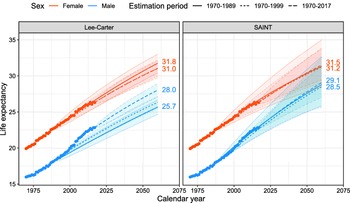


 Open access