


1 Introduction
Turbulent boundary-layer trailing-edge (TBL-TE) noise is one of the dominant sources of aerofoil self-noise in wind turbines (Brooks, Pope & Marcolini Reference Brooks, Pope and Marcolini1989; Wagner, Barei & Guidati Reference Wagner, Barei and Guidati1996). This source of noise limits both the installation of new wind turbines and the operational regimes of existing ones, thus reducing the power production and increasing the overall cost of energy (Oerlemans Reference Oerlemans2016).
With the goal of reducing TBL-TE noise of already existing wind turbines, many passive noise-mitigation solutions, based on the modification of the trailing-edge geometry with attachable add ons, have been proposed (Azarpeyvand, Gruber & Joseph Reference Azarpeyvand, Gruber and Joseph2013; Gruber, Joseph & Azarpeyvand Reference Gruber, Joseph and Azarpeyvand2013; Arce-León et al. Reference Arce-León, Avallone, Ragni and Pröbsting2016a ; Pringent, Buxton & Bruce Reference Pringent, Buxton and Bruce2017). Among others, sawtooth add ons are widely used for their simplicity of manufacturing and installation. More recently, Oerlemans (Reference Oerlemans2016) proposed a variation of the conventional sawtooth geometry, named as combed-sawtooth serration, with solid filaments filling the empty spaces between the teeth. This design showed additional 2 dB noise reduction during in-field measurements for the frequency range of practical interest.
The prediction of the scattered noise in presence of sawtooth serrations is not straightforward because of the complex three-dimensional flow generated by the spanwise varying geometry (Jones & Sandberg Reference Jones and Sandberg2012; Arce-León et al.
Reference Arce-León, Merino-Martínez, Ragni, Avallone and Snellen2016b
; Avallone, Pröbsting & Ragni Reference Avallone, Pröbsting and Ragni2016b
). Several analytical and semi-analytical models were developed to obtain reliable predictions for different trailing-edge shapes (Amiet Reference Amiet1976; Howe Reference Howe1991a
,Reference Howe
b
, Reference Howe1999; Azarpeyvand et al.
Reference Azarpeyvand, Gruber and Joseph2013; Lyu, Azarpeyvand & Sinayoko Reference Lyu, Azarpeyvand and Sinayoko2016; Stalnov, Chaitanya & Joseph Reference Stalnov, Chaitanya and Joseph2016). While predictions based upon analytical models require only details of the geometry, semi-analytical ones need additional information on the boundary-layer characteristics and on the spatial and temporal distribution of the surface pressure fluctuations (i.e. spectra
 $\unicode[STIX]{x1D6F7}_{pp}$
, spanwise correlation length
$\unicode[STIX]{x1D6F7}_{pp}$
, spanwise correlation length
 $l_{z}$
and convective velocity
$l_{z}$
and convective velocity
 $u_{c}$
). The first analytical solution for a serrated trailing edge was formulated by Howe (Howe Reference Howe1991a
,Reference Howe
b
). He showed that, under the assumption of frozen turbulence, for a semi-infinite flat plate with a serrated trailing edge, the noise reduction with respect to the straight trailing edge depends on the serration length (
$u_{c}$
). The first analytical solution for a serrated trailing edge was formulated by Howe (Howe Reference Howe1991a
,Reference Howe
b
). He showed that, under the assumption of frozen turbulence, for a semi-infinite flat plate with a serrated trailing edge, the noise reduction with respect to the straight trailing edge depends on the serration length (
 $2h$
) and wavelength (
$2h$
) and wavelength (
 $\unicode[STIX]{x1D706}$
). The model predicts an asymptotic noise reduction at high frequency of
$\unicode[STIX]{x1D706}$
). The model predicts an asymptotic noise reduction at high frequency of
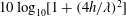 $10\log _{10}[1+(4h/\unicode[STIX]{x1D706})^{2}]$
dB. Even if this model is still widely used because of its simplicity, the predicted far-field noise spectra are typically not in agreement with measurements (Dassen et al.
Reference Dassen, Parchen, Bruggeman and Hagg1996; Parchen et al.
Reference Parchen, Hoffmans, Gordner and Braun1999; Oerlemans, Sijtsma & Lopez Reference Oerlemans, Sijtsma and Lopez2009; Gruber Reference Gruber2012; Gruber et al.
Reference Gruber, Joseph and Azarpeyvand2013; Chong & Vathylakis Reference Chong and Vathylakis2015; Arce-León et al.
Reference Arce-León, Avallone, Ragni and Pröbsting2016a
,Reference Arce-León, Merino-Martínez, Ragni, Avallone and Snellen
b
,Reference Arce-León, Ragni, Pröbsting, Scarano and Madsen
c
, Reference Arce-León, merino-Martinez, Ragni, Avallone, Scarano, Pröbsting, Snellen, Simons and Madsen2017; Avallone et al.
Reference Avallone, Pröbsting and Ragni2016b
); it over-predicts the maximum noise reduction and it does not predict the noise increase at frequencies higher than the so-called cross-over frequency
$10\log _{10}[1+(4h/\unicode[STIX]{x1D706})^{2}]$
dB. Even if this model is still widely used because of its simplicity, the predicted far-field noise spectra are typically not in agreement with measurements (Dassen et al.
Reference Dassen, Parchen, Bruggeman and Hagg1996; Parchen et al.
Reference Parchen, Hoffmans, Gordner and Braun1999; Oerlemans, Sijtsma & Lopez Reference Oerlemans, Sijtsma and Lopez2009; Gruber Reference Gruber2012; Gruber et al.
Reference Gruber, Joseph and Azarpeyvand2013; Chong & Vathylakis Reference Chong and Vathylakis2015; Arce-León et al.
Reference Arce-León, Avallone, Ragni and Pröbsting2016a
,Reference Arce-León, Merino-Martínez, Ragni, Avallone and Snellen
b
,Reference Arce-León, Ragni, Pröbsting, Scarano and Madsen
c
, Reference Arce-León, merino-Martinez, Ragni, Avallone, Scarano, Pröbsting, Snellen, Simons and Madsen2017; Avallone et al.
Reference Avallone, Pröbsting and Ragni2016b
); it over-predicts the maximum noise reduction and it does not predict the noise increase at frequencies higher than the so-called cross-over frequency
 $f^{\star }$
(Gruber et al.
Reference Gruber, Joseph and Azarpeyvand2013; Arce-León et al.
Reference Arce-León, merino-Martinez, Ragni, Avallone, Scarano, Pröbsting, Snellen, Simons and Madsen2017). More recently, Lyu et al. (Reference Lyu, Azarpeyvand and Sinayoko2016) developed a more accurate semi-analytical model that better estimates the maximum noise reduction with respect to experimental results. They individuated two non-dimensional parameters that affect noise reduction:
$f^{\star }$
(Gruber et al.
Reference Gruber, Joseph and Azarpeyvand2013; Arce-León et al.
Reference Arce-León, merino-Martinez, Ragni, Avallone, Scarano, Pröbsting, Snellen, Simons and Madsen2017). More recently, Lyu et al. (Reference Lyu, Azarpeyvand and Sinayoko2016) developed a more accurate semi-analytical model that better estimates the maximum noise reduction with respect to experimental results. They individuated two non-dimensional parameters that affect noise reduction:
 $k_{1}\times 2h$
and
$k_{1}\times 2h$
and
 $l_{z}(f)/\unicode[STIX]{x1D706}$
, where
$l_{z}(f)/\unicode[STIX]{x1D706}$
, where
 $k_{1}$
is the acoustic wavenumber in the chordwise direction and
$k_{1}$
is the acoustic wavenumber in the chordwise direction and
 $f$
is the frequency. When both quantities are larger than unity, far-field noise is significantly reduced. This means that the serration should be long enough to ensure a considerable phase difference between the scattered pressure waves along the edges. Furthermore, if the spatial range of the phase difference, i.e.
$f$
is the frequency. When both quantities are larger than unity, far-field noise is significantly reduced. This means that the serration should be long enough to ensure a considerable phase difference between the scattered pressure waves along the edges. Furthermore, if the spatial range of the phase difference, i.e.
 $\unicode[STIX]{x1D706}$
, is sufficiently small compared to the correlation length in the spanwise direction, radiated sound waves destructively interfere. However, some discrepancies with respect to experiments are still present, and they were attributed to the frozen-turbulence assumption by Arce-León et al. (Reference Arce-León, Merino-Martínez, Ragni, Avallone and Snellen2016b
) and Avallone et al. (Reference Avallone, Pröbsting and Ragni2016b
). As a matter of fact, Lyu et al. (Reference Lyu, Azarpeyvand and Sinayoko2016) concluded that the Chase’s turbulent boundary-layer spectrum model might represent a limitation to the applicability of the analytical solution particularly in the high-frequency range. For this purpose, a characterization of the statistical properties of the surface pressure fluctuations on the serrations and their frequency and spatial dependence is necessary.
$\unicode[STIX]{x1D706}$
, is sufficiently small compared to the correlation length in the spanwise direction, radiated sound waves destructively interfere. However, some discrepancies with respect to experiments are still present, and they were attributed to the frozen-turbulence assumption by Arce-León et al. (Reference Arce-León, Merino-Martínez, Ragni, Avallone and Snellen2016b
) and Avallone et al. (Reference Avallone, Pröbsting and Ragni2016b
). As a matter of fact, Lyu et al. (Reference Lyu, Azarpeyvand and Sinayoko2016) concluded that the Chase’s turbulent boundary-layer spectrum model might represent a limitation to the applicability of the analytical solution particularly in the high-frequency range. For this purpose, a characterization of the statistical properties of the surface pressure fluctuations on the serrations and their frequency and spatial dependence is necessary.
Experimental measurements showed that the intensity of the noise reduction is a function of the frequency and of the angle of attack. For a zero-angle-of-attack configuration, the largest reduction was measured for
 $5<St_{l}<15$
while almost no reduction was measured for
$5<St_{l}<15$
while almost no reduction was measured for
 $St_{l}>30$
, where
$St_{l}>30$
, where
 $St_{l}$
is the Strouhal number based on the airfoil chord and the free-stream velocity (Arce-León et al.
Reference Arce-León, Merino-Martínez, Ragni, Avallone and Snellen2016b
). The disagreement between analytical predictions and experiments has been recently investigated. Gruber (Reference Gruber2012) and Chong & Vathylakis (Reference Chong and Vathylakis2015) measured surface pressure fluctuations on serrations installed at the trailing edge of a flat plate. Quiescent conditions were maintained on one side of the plate. Both studies showed a larger spanwise magnitude-squared coherence of the surface pressure fluctuations
$St_{l}$
is the Strouhal number based on the airfoil chord and the free-stream velocity (Arce-León et al.
Reference Arce-León, Merino-Martínez, Ragni, Avallone and Snellen2016b
). The disagreement between analytical predictions and experiments has been recently investigated. Gruber (Reference Gruber2012) and Chong & Vathylakis (Reference Chong and Vathylakis2015) measured surface pressure fluctuations on serrations installed at the trailing edge of a flat plate. Quiescent conditions were maintained on one side of the plate. Both studies showed a larger spanwise magnitude-squared coherence of the surface pressure fluctuations
 $\unicode[STIX]{x1D6FE}^{2}$
with respect to the one measured for a straight trailing edge. In addition, Chong & Vathylakis (Reference Chong and Vathylakis2015) showed, by combining surface pressure and surface heat transfer measurements, the presence of pressure-driven edge-oriented vortices. They concluded that the angle between the local streamlines and the edge-oriented vortices affects the measured far-field noise. Similar observations on the role of the streamline curvature were reported by Arce-León et al. (Reference Arce-León, Ragni, Pröbsting, Scarano and Madsen2016c
), who measured with particle image velocimetry (PIV) the flow on a plane parallel to the serration surface retrofitted to a NACA 0018 aerofoil. However, by applying Howe’s model (Howe Reference Howe1991a
), corrected for the effective serration angle (i.e. the angle between the streamlines and the serration edge), they concluded that the streamline curvature correction cannot justify the measured noise reduction. A later study by Avallone et al. (Reference Avallone, Pröbsting and Ragni2016b
) showed that the flow field is three-dimensional with formation of large quasi-steady edge-oriented vortical structures in the empty space between teeth even at small angle of attack. These structures were attributed to the strong three-dimensional mixing layer across the serration edges. Considering the source term of the Poisson equation for the hydrodynamic pressure, they argued that the spectra of the near-wall pressure fluctuations strongly vary along the serration surface, thus making the assumption of frozen turbulence no longer valid. More precisely, they showed that the convective velocity of the streamwise velocity component increases from the root to the tip while the spanwise correlation length of the spanwise velocity component decreases from the root to the tip. They further showed that noise is mainly generated at the root of the serrations. Based on the previous observations, Avallone, van der Velden & Ragni (Reference Avallone, van der Velden and Ragni2017) designed the so-called iron-shaped serration. They obtained additional
$\unicode[STIX]{x1D6FE}^{2}$
with respect to the one measured for a straight trailing edge. In addition, Chong & Vathylakis (Reference Chong and Vathylakis2015) showed, by combining surface pressure and surface heat transfer measurements, the presence of pressure-driven edge-oriented vortices. They concluded that the angle between the local streamlines and the edge-oriented vortices affects the measured far-field noise. Similar observations on the role of the streamline curvature were reported by Arce-León et al. (Reference Arce-León, Ragni, Pröbsting, Scarano and Madsen2016c
), who measured with particle image velocimetry (PIV) the flow on a plane parallel to the serration surface retrofitted to a NACA 0018 aerofoil. However, by applying Howe’s model (Howe Reference Howe1991a
), corrected for the effective serration angle (i.e. the angle between the streamlines and the serration edge), they concluded that the streamline curvature correction cannot justify the measured noise reduction. A later study by Avallone et al. (Reference Avallone, Pröbsting and Ragni2016b
) showed that the flow field is three-dimensional with formation of large quasi-steady edge-oriented vortical structures in the empty space between teeth even at small angle of attack. These structures were attributed to the strong three-dimensional mixing layer across the serration edges. Considering the source term of the Poisson equation for the hydrodynamic pressure, they argued that the spectra of the near-wall pressure fluctuations strongly vary along the serration surface, thus making the assumption of frozen turbulence no longer valid. More precisely, they showed that the convective velocity of the streamwise velocity component increases from the root to the tip while the spanwise correlation length of the spanwise velocity component decreases from the root to the tip. They further showed that noise is mainly generated at the root of the serrations. Based on the previous observations, Avallone, van der Velden & Ragni (Reference Avallone, van der Velden and Ragni2017) designed the so-called iron-shaped serration. They obtained additional
 $2$
dB noise reduction with respect to the conventional sawtooth serration. Further improvements could be obtained with a better understanding of the effects of serrations on the wall pressure statistics. However, it is very difficult to measure the surface pressure fluctuations on thin surfaces without perturbing the flow (Gruber Reference Gruber2012; Chong & Vathylakis Reference Chong and Vathylakis2015).
$2$
dB noise reduction with respect to the conventional sawtooth serration. Further improvements could be obtained with a better understanding of the effects of serrations on the wall pressure statistics. However, it is very difficult to measure the surface pressure fluctuations on thin surfaces without perturbing the flow (Gruber Reference Gruber2012; Chong & Vathylakis Reference Chong and Vathylakis2015).
Computations might help in overcoming the experimental limitations mentioned above. Numerical analyses studied the flow organization around trailing-edge serrations (Arina et al. Reference Arina, Della Ratta Rinaldi, Iob and Torzo2012; Jones & Sandberg Reference Jones and Sandberg2012; Sanjose et al. Reference Sanjose, Meon, Masson and Moreau2014; Kim, Haeri & Joseph Reference Kim, Haeri and Joseph2016; van der Velden, van Zuijlen & Ragni Reference van der Velden, van Zuijlen and Ragni2016b ; Merino-Martinez et al. Reference Merino-Martinez, van der Velden, Avallone and Ragni2017; van der Velden & Oerlemans Reference van der Velden and Oerlemans2017). Among others, Jones & Sandberg (Reference Jones and Sandberg2012) analysed the flow over a NACA 0012 retrofitted with trailing-edge serrations and a split plate. In this study, the boundary layer was not forced to turbulent and the effect of the flow separation/reattachment at the suction side did not allow to isolate the contribution of TBL-TE noise. However, they showed that the flow is three-dimensional with the presence of horseshoe vortices in the empty space between the teeth, which were promoting a seeping motion from the suction to the pressure side. Furthermore, they found that the wake evolves faster toward a more spanwise structure-dominated flow in the presence of trailing-edge serrations. They concluded that the far-field noise levels are affected only by a modification of the edge scattering process, and potentially by a different hydrodynamic behaviour in the direct vicinity of the serrations. However, no further link between the hydrodynamic flow features and the scattered far-field noise was proposed.
The goal of this manuscript is to elucidate the relation between hydrodynamic flow features and the far-field noise. For this reason, the most relevant parameters responsible for noise radiation are carefully investigated. Since it is experimentally challenging to measure pressure on the surface of the serrations without affecting the flow field, a computational approach is chosen. A characterization of the surface pressure fluctuations allows improving the existing analytical approaches. For this reason, the flow over a serrated trailing edge retrofitted to a NACA 0018 aerofoil at zero angle of attack is computed by solving the explicit, transient, compressible lattice Boltzmann equation, while the acoustic far field is obtained by means of the Ffowcs Williams and Hawkings (FW–H) acoustic analogy (Ffowcs-Williams & Hawkings Reference Ffowcs-Williams and Hawkings1969). The configuration is a replica of the experiments performed by Arce-León et al. (Reference Arce-León, Merino-Martínez, Ragni, Avallone and Snellen2016b ) to which the computational results are compared. The zero-angle-of-attack configuration is chosen because it allows isolating the effect of the serration loading on the hydrodynamic flow field and the radiated noise. This case represents the simplest but unavoidable test bench for analytical models. However, in order to compare with the state-of-the-art serration geometry, combed-sawtooth serrations are further studied. A first analysis of this configurations was carried out earlier by van der Velden & Oerlemans (Reference van der Velden and Oerlemans2017) who showed that this geometry mitigates the flow unsteadiness at root, thus being beneficial for trailing-edge noise reduction.
In the following, the computational methodology is discussed in § 2. A brief discussion of the two different computational test cases is given in § 3. The computational set-up is validated in § 4 by means of a grid convergence study and comparison with experimental data, both in terms of mean flow features and far-field noise. The acoustic far-field results for all configurations are then discussed in § 5. In the same section, a detailed analysis of the source distribution along the serrations is performed. Finally, the instantaneous flow field and the integral parameters of the surface pressure fluctuations are investigated in §§ 6 and 7. The main findings of this work are summarized in the conclusions.
2 Computational method
2.1 Flow solver
The lattice Boltzmann (LB) method is used to compute the flow field because it was shown to be accurate and efficient for trailing-edge noise prediction in presence of complex flow problems (van der Velden et al. Reference van der Velden, Probsting, van Zuijlen, de Jong, Guan and Morris2016; van der Velden & Oerlemans Reference van der Velden and Oerlemans2017). The commercial software PowerFLOW 5.3b is adopted. It solves the discrete LB equation for a finite number of directions. For a detailed description of the method, the reader can refer to Succi (Reference Succi2001). The LB method determines the macroscopic flow variables starting from the mesoscopic kinetic equation, i.e. the LB equation. The discretization used for this particular application consists of 19 discrete velocities in three dimensions (D3Q19), involving a third-order truncation of the Chapman–Enskog expansion. It was shown that this scheme accurately approximates the Navier–Stokes equations for a perfect gas at low Mach number in isothermal conditions (Chen, Chen & Matthaeus Reference Chen, Chen and Matthaeus1992). The distribution of particles is solved by means of the LB equation on a Cartesian mesh, known as a lattice. An explicit time integration and a collision model are used. The LB equation can then be written as:
 $$\begin{eqnarray}\displaystyle g_{i}(\boldsymbol{x}+\boldsymbol{c}_{i}\unicode[STIX]{x0394}t,t+\unicode[STIX]{x0394}t)-g_{i}(\boldsymbol{x},t)=C_{i}(\boldsymbol{x},t), & & \displaystyle\end{eqnarray}$$
where
 $g_{i}$
is the particle distribution function along the
$g_{i}$
is the particle distribution function along the
 $i$
th lattice direction. It statistically describes the particle motion at a position
$i$
th lattice direction. It statistically describes the particle motion at a position
 $\boldsymbol{x}$
with a discrete velocity
$\boldsymbol{x}$
with a discrete velocity
 $\boldsymbol{c}_{i}$
in the
$\boldsymbol{c}_{i}$
in the
 $i$
direction at time
$i$
direction at time
 $t$
.
$t$
.
 $\boldsymbol{c}_{i}\unicode[STIX]{x0394}t$
and
$\boldsymbol{c}_{i}\unicode[STIX]{x0394}t$
and
 $\unicode[STIX]{x0394}t$
are space and time increments, respectively.
$\unicode[STIX]{x0394}t$
are space and time increments, respectively.
 $C_{i}(\boldsymbol{x},t)$
is the collision term for which the Bhatnagar–Gross–Krook (BGK) model (Bhatnagar, Gross & Krook Reference Bhatnagar, Gross and Krook1954; Chen et al.
Reference Chen, Chen and Matthaeus1992) is adopted because of its simplicity:
$C_{i}(\boldsymbol{x},t)$
is the collision term for which the Bhatnagar–Gross–Krook (BGK) model (Bhatnagar, Gross & Krook Reference Bhatnagar, Gross and Krook1954; Chen et al.
Reference Chen, Chen and Matthaeus1992) is adopted because of its simplicity:
 $$\begin{eqnarray}\displaystyle C_{i}(\boldsymbol{x},t)=-\frac{\unicode[STIX]{x0394}t}{\unicode[STIX]{x1D70F}}[g_{i}(\boldsymbol{x},t)-g_{i}^{eq}(\boldsymbol{x},t)], & & \displaystyle\end{eqnarray}$$
where
 $\unicode[STIX]{x1D70F}$
is the relaxation time and
$\unicode[STIX]{x1D70F}$
is the relaxation time and
 $g_{i}^{eq}$
is the local equilibrium distribution function. For small Mach number flows the equilibrium distribution of Maxwell–Boltzmann is conventionally used (Chen et al.
Reference Chen, Chen and Matthaeus1992). It is approximated by a second-order expansion as:
$g_{i}^{eq}$
is the local equilibrium distribution function. For small Mach number flows the equilibrium distribution of Maxwell–Boltzmann is conventionally used (Chen et al.
Reference Chen, Chen and Matthaeus1992). It is approximated by a second-order expansion as:
 $$\begin{eqnarray}\displaystyle g_{i}^{eq}=\unicode[STIX]{x1D70C}\unicode[STIX]{x1D714}_{i}\left[1+\frac{\boldsymbol{c}_{i}\boldsymbol{u}}{c_{s}^{2}}+\frac{(\boldsymbol{c}_{i}\boldsymbol{u})^{2}}{2c_{s}^{4}}+\frac{|\boldsymbol{u}|^{2}}{2c_{s}^{2}}\right], & & \displaystyle\end{eqnarray}$$
where
 $\unicode[STIX]{x1D714}_{i}$
are the fixed weight functions, dependent on the velocity discretization model D3Q19 (Chen et al.
Reference Chen, Chen and Matthaeus1992), and
$\unicode[STIX]{x1D714}_{i}$
are the fixed weight functions, dependent on the velocity discretization model D3Q19 (Chen et al.
Reference Chen, Chen and Matthaeus1992), and
 $c_{s}=1/\sqrt{3}$
is the non-dimensional speed of sound in lattice units. The macroscopic flow quantities density
$c_{s}=1/\sqrt{3}$
is the non-dimensional speed of sound in lattice units. The macroscopic flow quantities density
 $\unicode[STIX]{x1D70C}$
and velocity
$\unicode[STIX]{x1D70C}$
and velocity
 $\boldsymbol{u}$
, are obtained by discrete integration of the microscopic quantities weighted by the distribution function over the state space:
$\boldsymbol{u}$
, are obtained by discrete integration of the microscopic quantities weighted by the distribution function over the state space:
 $$\begin{eqnarray}\displaystyle \unicode[STIX]{x1D70C}(\boldsymbol{x},t)=\mathop{\sum }_{i}g_{i}(\boldsymbol{x},t),\quad \unicode[STIX]{x1D70C}\boldsymbol{u}(\boldsymbol{x},t)=\mathop{\sum }_{i}\boldsymbol{c}_{i}g_{i}(\boldsymbol{x},t). & & \displaystyle\end{eqnarray}$$
The dimensionless kinematic viscosity
 $\unicode[STIX]{x1D708}$
is related to the relaxation time following Chen et al. (Reference Chen, Chen and Matthaeus1992):
$\unicode[STIX]{x1D708}$
is related to the relaxation time following Chen et al. (Reference Chen, Chen and Matthaeus1992):
 $$\begin{eqnarray}\displaystyle \unicode[STIX]{x1D708}=c_{s}^{2}\left(\unicode[STIX]{x1D70F}-\frac{\unicode[STIX]{x0394}t}{2}\right). & & \displaystyle\end{eqnarray}$$
A very large eddy simulation (VLES) model is implemented to take into account the effect of the sub-grid unresolved scales of turbulence. Following Yakhot & Orszag (Reference Yakhot and Orszag1986), a two-equation
 $k{-}\unicode[STIX]{x1D716}$
renormalization group (RNG) is used to compute a turbulent relaxation time that is added to the viscous relaxation time:
$k{-}\unicode[STIX]{x1D716}$
renormalization group (RNG) is used to compute a turbulent relaxation time that is added to the viscous relaxation time:
 $$\begin{eqnarray}\displaystyle \unicode[STIX]{x1D70F}_{eff}=\unicode[STIX]{x1D70F}+C_{\unicode[STIX]{x1D707}}\frac{k^{2}/\unicode[STIX]{x1D716}}{(1+\unicode[STIX]{x1D702}^{2})^{1/2}}, & & \displaystyle\end{eqnarray}$$
where
 $C_{\unicode[STIX]{x1D707}}=0.09$
and
$C_{\unicode[STIX]{x1D707}}=0.09$
and
 $\unicode[STIX]{x1D702}$
are a combination of the local strain, local vorticity and local helicity parameters. The term
$\unicode[STIX]{x1D702}$
are a combination of the local strain, local vorticity and local helicity parameters. The term
 $\unicode[STIX]{x1D702}$
allows to mitigate the sub-grid scale viscosity in presence of large resolved vortical structures.
$\unicode[STIX]{x1D702}$
allows to mitigate the sub-grid scale viscosity in presence of large resolved vortical structures.
In order to reduce the computational cost, a pressure-gradient extended wall model (PGE-WM) is used to approximate the no-slip boundary condition on solid walls (Teixeria Reference Teixeria1998; Wilcox Reference Wilcox2006). The model is based on the extension of the generalized law-of-the-wall model (Launder & Spalding Reference Launder and Spalding1974) to take into account the effect of pressure gradient. The expression of the PGE-WM is:
 $$\begin{eqnarray}\displaystyle u^{+}=\frac{1}{\unicode[STIX]{x1D705}}\ln \left(\frac{y^{+}}{A}\right)+B, & & \displaystyle\end{eqnarray}$$
where
 $$\begin{eqnarray}\displaystyle B=5.0,\quad \unicode[STIX]{x1D705}=0.41,\quad y^{+}=\frac{u_{\unicode[STIX]{x1D70F}}y}{\unicode[STIX]{x1D708}}, & & \displaystyle\end{eqnarray}$$
and where
 $A$
is a function of the pressure gradient. It captures the physical consequence that the velocity profile slows down and so expands, due to the presence of the pressure gradient, at least at the early stage of the development. The expression of
$A$
is a function of the pressure gradient. It captures the physical consequence that the velocity profile slows down and so expands, due to the presence of the pressure gradient, at least at the early stage of the development. The expression of
 $A$
is:
$A$
is:
 $$\begin{eqnarray}\displaystyle A=1+\frac{f\left|\displaystyle \frac{\text{d}p}{\text{d}s}\right|}{\unicode[STIX]{x1D70F}_{w}},\quad \hat{\boldsymbol{u}}_{\boldsymbol{s}}\boldsymbol{\cdot }\frac{\text{d}p}{\text{d}s}>0, & & \displaystyle\end{eqnarray}$$
 $$\begin{eqnarray}\displaystyle A=1,\quad \text{otherwise}. & & \displaystyle\end{eqnarray}$$
In the equations,
 $\unicode[STIX]{x1D70F}_{w}$
is the wall shear stress,
$\unicode[STIX]{x1D70F}_{w}$
is the wall shear stress,
 $\text{d}p/\text{d}s$
is the streamwise pressure gradient,
$\text{d}p/\text{d}s$
is the streamwise pressure gradient,
 $\hat{\boldsymbol{u}}_{\boldsymbol{s}}$
is the unit vector of the local slip velocity and
$\hat{\boldsymbol{u}}_{\boldsymbol{s}}$
is the unit vector of the local slip velocity and
 $f$
is a length scale equal to the size the unresolved near-wall region. These equations are iteratively solved from the first cell close to the wall in order to specify the boundary conditions of the turbulence model. For this purpose, a slip algorithm (Chen, Teixeira & Molvig Reference Chen, Teixeira and Molvig1998), obtained as generalization of a bounce back and specular reflection process, is used.
$f$
is a length scale equal to the size the unresolved near-wall region. These equations are iteratively solved from the first cell close to the wall in order to specify the boundary conditions of the turbulence model. For this purpose, a slip algorithm (Chen, Teixeira & Molvig Reference Chen, Teixeira and Molvig1998), obtained as generalization of a bounce back and specular reflection process, is used.
2.2 Noise computations
The compressible and time-dependent nature of the transient computed solution together with the low dissipation and dispersion properties of the LB scheme (Bres, Perot & Freed Reference Bres, Perot and Freed2009) allow extracting the sound pressure field directly in the near field up to a cutoff frequency corresponding to approximately 15 voxels per acoustic wavelength.
In the far field, noise is computed by using the Ffowcs-Williams & Hawkings (Reference Ffowcs-Williams and Hawkings1969) (FW–H) equation. The formulation 1A, developed by Farassat & Succi (Reference Farassat and Succi1980), extended to a convective wave equation, is used in this study (Bres et al. Reference Bres, Perot and Freed2009). The formulation is implemented in the time domain using a source-time dominant algorithm (Casalino Reference Casalino2003). Integrations are performed on the surface of the aerofoil where the unsteady pressure is recorded with the highest frequency rate available on the finest mesh resolution level. As a consequence, acoustic dipoles distributed on the surface of the aerofoil are the only source terms of interest (Curle Reference Curle1955) and the nonlinear contribution related to the turbulent fluctuations in the wake of the aerofoil is neglected.

Figure 1. Aerofoil, serration geometries and dimensions.
3 Computational test cases
A NACA 0018 aerofoil with a chord of
 $l=0.2~\text{m}$
and span of
$l=0.2~\text{m}$
and span of
 $b=0.08~\text{m}$
(
$b=0.08~\text{m}$
(
 $b=0.4l$
) is investigated (figure 1). The free-stream velocity is
$b=0.4l$
) is investigated (figure 1). The free-stream velocity is
 $u_{\infty }=20~\text{m}~\text{s}^{-1}$
, corresponding to a free-stream Mach number
$u_{\infty }=20~\text{m}~\text{s}^{-1}$
, corresponding to a free-stream Mach number
 $M_{\infty }=0.06$
, and a chord-based Reynolds number of
$M_{\infty }=0.06$
, and a chord-based Reynolds number of
 $Re_{l}=280\,000$
. The free-stream turbulence intensity is set to 0.1 %. The angle of attack is
$Re_{l}=280\,000$
. The free-stream turbulence intensity is set to 0.1 %. The angle of attack is
 $\unicode[STIX]{x1D6FC}=0$
deg. The wind-tunnel model and the free-stream conditions are chosen as in the experiments of Arce-León et al. (Reference Arce-León, Merino-Martínez, Ragni, Avallone and Snellen2016b
), which measurements are used as reference. Similarly to the experiments, boundary-layer transition to turbulence is forced. In this case, a zig–zag strip (van der Velden et al.
Reference van der Velden, van Zuijlen, de Jong and Ragni2017) of height
$\unicode[STIX]{x1D6FC}=0$
deg. The wind-tunnel model and the free-stream conditions are chosen as in the experiments of Arce-León et al. (Reference Arce-León, Merino-Martínez, Ragni, Avallone and Snellen2016b
), which measurements are used as reference. Similarly to the experiments, boundary-layer transition to turbulence is forced. In this case, a zig–zag strip (van der Velden et al.
Reference van der Velden, van Zuijlen, de Jong and Ragni2017) of height
 $t_{trip}=0.6~\text{mm}$
(
$t_{trip}=0.6~\text{mm}$
(
 $t_{trip}=0.003l$
), amplitude
$t_{trip}=0.003l$
), amplitude
 $l_{trip}=3~\text{mm}$
(
$l_{trip}=3~\text{mm}$
(
 $l_{trip}=0.015l$
) and wavelength
$l_{trip}=0.015l$
) and wavelength
 $b_{trip}=3~\text{mm}$
(
$b_{trip}=3~\text{mm}$
(
 $b_{trip}=0.015l$
) on both aerofoil sides at
$b_{trip}=0.015l$
) on both aerofoil sides at
 $x=-0.8l$
, i.e. 20 % of the chord, is used. The height of the zig–zag strip corresponds to approximately half the local incoming laminar boundary-layer thickness (
$x=-0.8l$
, i.e. 20 % of the chord, is used. The height of the zig–zag strip corresponds to approximately half the local incoming laminar boundary-layer thickness (
 $\unicode[STIX]{x1D6FF}_{0}$
). The aerofoil is retrofitted with a straight, a sawtooth and a combed-sawtooth trailing edge. Serrations have length
$\unicode[STIX]{x1D6FF}_{0}$
). The aerofoil is retrofitted with a straight, a sawtooth and a combed-sawtooth trailing edge. Serrations have length
 $2h=0.04~\text{m}$
(
$2h=0.04~\text{m}$
(
 $2h=0.2l$
) and wavelength
$2h=0.2l$
) and wavelength
 $\unicode[STIX]{x1D706}=0.02~\text{m}$
(
$\unicode[STIX]{x1D706}=0.02~\text{m}$
(
 $\unicode[STIX]{x1D706}=0.1l$
), resulting in an aspect ratio of
$\unicode[STIX]{x1D706}=0.1l$
), resulting in an aspect ratio of
 $2h/\unicode[STIX]{x1D706}=2$
. The length of the serration was chosen to be approximately equal to four times the length of the boundary-layer thickness based on 95 % of the free-stream velocity (based on XFOIL computations (Drela Reference Drela and Mueller1989)) for the tested Reynolds number. Combed-sawtooth serrations have the same solid geometry and filaments with both thickness and clearance of
$2h/\unicode[STIX]{x1D706}=2$
. The length of the serration was chosen to be approximately equal to four times the length of the boundary-layer thickness based on 95 % of the free-stream velocity (based on XFOIL computations (Drela Reference Drela and Mueller1989)) for the tested Reynolds number. Combed-sawtooth serrations have the same solid geometry and filaments with both thickness and clearance of
 $d=0.5~\text{mm}$
(
$d=0.5~\text{mm}$
(
 $d=0.0025l$
). Both trailing-edge add ons have the same thickness of the straight trailing edge equal to 1 mm (
$d=0.0025l$
). Both trailing-edge add ons have the same thickness of the straight trailing edge equal to 1 mm (
 $t_{ser}=0.005l$
). A total of
$t_{ser}=0.005l$
). A total of
 $4$
serrations are present along the span. A sketch of the geometries and of the adopted Cartesian coordinate system is shown in figure 1. The
$4$
serrations are present along the span. A sketch of the geometries and of the adopted Cartesian coordinate system is shown in figure 1. The
 $z$
-axis coincides with the aerofoil trailing edge; the
$z$
-axis coincides with the aerofoil trailing edge; the
 $y$
-axis is perpendicular to the surface of the serrations; and the
$y$
-axis is perpendicular to the surface of the serrations; and the
 $x$
-axis is aligned with the chord of the aerofoil. The origin is set at the location of the baseline aerofoil with straight trailing edge, such that the
$x$
-axis is aligned with the chord of the aerofoil. The origin is set at the location of the baseline aerofoil with straight trailing edge, such that the
 $x$
-axis is oriented along the serration centreline.
$x$
-axis is oriented along the serration centreline.
The simulation domain is a box of length equal to
 $12l$
in both streamwise and wall-normal directions and
$12l$
in both streamwise and wall-normal directions and
 $b$
in the spanwise direction. Periodic boundary conditions are applied on the lateral faces of the simulation domain. Outside a circular refinement zone of diameter equal to
$b$
in the spanwise direction. Periodic boundary conditions are applied on the lateral faces of the simulation domain. Outside a circular refinement zone of diameter equal to
 $10l$
an anechoic outer layer is used to damp out the outward radiating and the inward reflected acoustic waves. A total of 10 mesh refinement regions with resolution factor equal to 2 are employed. This guarantees that, at the trailing-edge location, the first near-wall cell is located at approximately
$10l$
an anechoic outer layer is used to damp out the outward radiating and the inward reflected acoustic waves. A total of 10 mesh refinement regions with resolution factor equal to 2 are employed. This guarantees that, at the trailing-edge location, the first near-wall cell is located at approximately
 $3.9\times 10^{-4}l$
, i.e. inside the viscous sub-layer. It results in a resolution of about
$3.9\times 10^{-4}l$
, i.e. inside the viscous sub-layer. It results in a resolution of about
 $y^{+}=3$
around the trailing edge in all the directions. The rest of the aerofoil boundary is modelled with one coarser level of resolution. In total, approximately
$y^{+}=3$
around the trailing edge in all the directions. The rest of the aerofoil boundary is modelled with one coarser level of resolution. In total, approximately
 $150$
million cubic cells (voxels) are used to discretize the problem. A mesh resolution study has been carried out in order to verify the convergence of the boundary-layer characteristics at the trailing-edge location and the far-field noise. The accuracy of the discretization is also validated comparing the computational results with experimental data. Details are described in § 4. The flow-simulation time is 0.3 s (30 flow passes) requiring
$150$
million cubic cells (voxels) are used to discretize the problem. A mesh resolution study has been carried out in order to verify the convergence of the boundary-layer characteristics at the trailing-edge location and the far-field noise. The accuracy of the discretization is also validated comparing the computational results with experimental data. Details are described in § 4. The flow-simulation time is 0.3 s (30 flow passes) requiring
 $6300$
CPU hours on a Linux Xeon E5-2690 2.9 GHz platform.
$6300$
CPU hours on a Linux Xeon E5-2690 2.9 GHz platform.
The physical time step, corresponding to a Courant–Friedrichs–Lewy (CFL) number of 1 in the finest mesh resolution level, is
 $1.3\times 10^{-7}~\text{s}$
. The unsteady pressure on the surface of the aerofoil is sampled with a frequency of 30 kHz (
$1.3\times 10^{-7}~\text{s}$
. The unsteady pressure on the surface of the aerofoil is sampled with a frequency of 30 kHz (
 $St_{l}=fl/u_{\infty }=300$
) for a physical time of 0.2 s (equals to
$St_{l}=fl/u_{\infty }=300$
) for a physical time of 0.2 s (equals to
 $20$
aerofoil flow passes). Given the periodicity of the flow for the different serrations, the computed fields are spatially averaged along the spanwise direction, as well as over the top and bottom sides of the serration. The average is carried out along points with the same relative location with respect to the serration root. This procedure reduces the uncertainty on the mean values as well as increases the number of samples available for the spectra evaluation (Jones & Sandberg Reference Jones and Sandberg2012).
$20$
aerofoil flow passes). Given the periodicity of the flow for the different serrations, the computed fields are spatially averaged along the spanwise direction, as well as over the top and bottom sides of the serration. The average is carried out along points with the same relative location with respect to the serration root. This procedure reduces the uncertainty on the mean values as well as increases the number of samples available for the spectra evaluation (Jones & Sandberg Reference Jones and Sandberg2012).
4 Grid resolution study and comparison with experiments
Grid resolution studies are carried out to verify convergence of both the hydrodynamic and acoustic fields. Four grid resolutions are investigated: coarse (
 $y^{+}=12$
), medium (
$y^{+}=12$
), medium (
 $y^{+}=6$
), fine (
$y^{+}=6$
), fine (
 $y^{+}=3$
) and very fine (
$y^{+}=3$
) and very fine (
 $y^{+}=1.5$
). This is achieved by doubling the resolution of each refinement region. The boundary-layer thickness
$y^{+}=1.5$
). This is achieved by doubling the resolution of each refinement region. The boundary-layer thickness
 $\unicode[STIX]{x1D6FF}$
for the straight trailing edge at
$\unicode[STIX]{x1D6FF}$
for the straight trailing edge at
 $x/l=-0.005$
is used as integral hydrodynamic parameter for the convergence analysis. It is plotted versus the grid factor
$x/l=-0.005$
is used as integral hydrodynamic parameter for the convergence analysis. It is plotted versus the grid factor
 $N^{-2/3}$
in figure 2, where
$N^{-2/3}$
in figure 2, where
 $N$
is the total number of voxels.
$N$
is the total number of voxels.

Figure 2. Boundary-layer thickness at
 $x/l=-0.005$
for different mesh sizes. The dashed line reports the Richardson extrapolation, while the square tick indicates the resolution adopted throughout the manuscript.
$x/l=-0.005$
for different mesh sizes. The dashed line reports the Richardson extrapolation, while the square tick indicates the resolution adopted throughout the manuscript.
Figure 2 shows that convergence towards a boundary-layer thickness of 9.3 mm is obtained for the fine resolution case (
 $y^{+}=3$
). It is further verified that the shape factor
$y^{+}=3$
). It is further verified that the shape factor
 $H=\unicode[STIX]{x1D6FF}^{\star }/\unicode[STIX]{x1D703}$
is equal to 2.2, as in the experiments. The Richardson extrapolation with a refinement ratio of
$H=\unicode[STIX]{x1D6FF}^{\star }/\unicode[STIX]{x1D703}$
is equal to 2.2, as in the experiments. The Richardson extrapolation with a refinement ratio of
 $r=2$
and order of convergence of
$r=2$
and order of convergence of
 $p=3$
(discarding the coarsest mesh), plotted as dashed line in figure 2, confirms convergence of the hydrodynamic flow field. An additional check of the grid convergence is carried out via the grid convergence index (
$p=3$
(discarding the coarsest mesh), plotted as dashed line in figure 2, confirms convergence of the hydrodynamic flow field. An additional check of the grid convergence is carried out via the grid convergence index (
 $GCI$
). It is
$GCI$
). It is
 $GCI_{2,3}=2.36\,\%$
and
$GCI_{2,3}=2.36\,\%$
and
 $GCI_{1,2}=0.30\,\%$
for both the fine and very fine grid resolutions, respectively. Their ratio, computed as in equation (4.1), is approximately equal to 1. It indicates a grid-dependent solution (Roache Reference Roache1994) and ensures that both grids are in the asymptotic range of convergence.
$GCI_{1,2}=0.30\,\%$
for both the fine and very fine grid resolutions, respectively. Their ratio, computed as in equation (4.1), is approximately equal to 1. It indicates a grid-dependent solution (Roache Reference Roache1994) and ensures that both grids are in the asymptotic range of convergence.
 $$\begin{eqnarray}\displaystyle \frac{GCI_{2,3}}{r^{p}\times GCI_{1,2}}=0.98\approx 1. & & \displaystyle\end{eqnarray}$$
Based on the previous considerations, the fine grid resolution (
 $y^{+}=3$
) is used in the rest of the study (solid square in figure 2). The resulting boundary-layer parameters for the selected grid resolution and for the straight trailing edge are shown in table 1.
$y^{+}=3$
) is used in the rest of the study (solid square in figure 2). The resulting boundary-layer parameters for the selected grid resolution and for the straight trailing edge are shown in table 1.
Table 1. Boundary-layer parameters for the straight trailing edge at
 $x/l=-0.005$
for the fine grid resolution (
$x/l=-0.005$
for the fine grid resolution (
 $y^{+}=3$
).
$y^{+}=3$
).


Figure 3. (a) Time-averaged, root-mean-square of the (b) streamwise and of (c) the wall-normal velocity components. Profiles at different locations along the edge for the straight and sawtooth configurations. Experimental PIV data for the serrated case (circles) are extracted from Arce-León et al. (Reference Arce-León, Merino-Martínez, Ragni, Avallone and Snellen2016b
). The locations along the serration, indicated in the legend, are: (yellow)
 $x/2h=0$
, (green)
$x/2h=0$
, (green)
 $x/2h=0.5$
and (light blue)
$x/2h=0.5$
and (light blue)
 $x/2h=1$
; the boundary layer for the straight trailing edge is reported in purple.
$x/2h=1$
; the boundary layer for the straight trailing edge is reported in purple.
Results from the selected grid resolution are further compared against PIV experimental results (Arce-León et al.
Reference Arce-León, Merino-Martínez, Ragni, Avallone and Snellen2016b
). A description of the experimental set-up is reported in appendix A. Time-averaged mean and turbulent velocity fluctuations (i.e. the root-mean-square) in the boundary layer for both the straight and the sawtooth trailing edges are plotted (figure 3). For the latter, three streamwise locations along the edge are investigated:
 $x/2h=0$
,
$x/2h=0$
,
 $x/2h=0.5$
and
$x/2h=0.5$
and
 $x/2h=1$
. In figure 3, the wall-normal location
$x/2h=1$
. In figure 3, the wall-normal location
 $y$
and the velocity statistics are respectively non-dimensionalized with respect to
$y$
and the velocity statistics are respectively non-dimensionalized with respect to
 $\unicode[STIX]{x1D6FF}$
and
$\unicode[STIX]{x1D6FF}$
and
 $u_{e}$
(i.e. the edge velocity) taken at
$u_{e}$
(i.e. the edge velocity) taken at
 $x/2h=0$
for the straight trailing edge (table 1).
$x/2h=0$
for the straight trailing edge (table 1).
A very good agreement is found between experimental measurements and computational results for both the mean and turbulent velocity profiles. The intensity of the velocity fluctuations is also well captured, thus suggesting that the adopted zig–zag turbolator creates a turbulent boundary layer similar to the experimental one. Data confirm that the presence of the sawtooth trailing edge weakly affects the flow upstream. Computational results further capture the decrease of the boundary-layer thickness towards the tip of the serration and the consequent increase of the near-wall streamwise velocity. On the other hand, the root-mean-square (r.m.s.) of both the streamwise
 $\overline{u^{\prime }u^{\prime }}$
and wall-normal
$\overline{u^{\prime }u^{\prime }}$
and wall-normal
 $\overline{v^{\prime }v^{\prime }}$
velocity components decreases in intensity toward the sawtooth tip. The location of the maximum
$\overline{v^{\prime }v^{\prime }}$
velocity components decreases in intensity toward the sawtooth tip. The location of the maximum
 $\overline{u^{\prime }u^{\prime }}$
moves toward the outer edge of the boundary layer at downstream locations, while the location of the maximum
$\overline{u^{\prime }u^{\prime }}$
moves toward the outer edge of the boundary layer at downstream locations, while the location of the maximum
 $\overline{v^{\prime }v^{\prime }}$
is constant at approximately
$\overline{v^{\prime }v^{\prime }}$
is constant at approximately
 $y/\unicode[STIX]{x1D6FF}\approx 0.3$
. Similar flow features were also found in other experimental studies (Gruber Reference Gruber2012; Avallone et al.
Reference Avallone, Pröbsting and Ragni2016b
).
$y/\unicode[STIX]{x1D6FF}\approx 0.3$
. Similar flow features were also found in other experimental studies (Gruber Reference Gruber2012; Avallone et al.
Reference Avallone, Pröbsting and Ragni2016b
).

Figure 4. Far-field pressure spectra (a)
 $\unicode[STIX]{x1D6F7}_{aa}$
and (b)
$\unicode[STIX]{x1D6F7}_{aa}$
and (b)
 $\unicode[STIX]{x0394}\unicode[STIX]{x1D6F7}_{aa}$
with respect to the straight trailing edge. Experimental data are taken from Arce-León et al. (Reference Arce-León, Merino-Martínez, Ragni, Avallone and Snellen2016b
).
$\unicode[STIX]{x0394}\unicode[STIX]{x1D6F7}_{aa}$
with respect to the straight trailing edge. Experimental data are taken from Arce-León et al. (Reference Arce-León, Merino-Martínez, Ragni, Avallone and Snellen2016b
).
The comparison with the experiments is further extended to the far-field noise to assess the suitability of the selected computational grid. The far-field acoustic spectra, obtained with the FW–H analogy described in § 2.2, are compared with microphone array measurements (Arce-León et al.
Reference Arce-León, Merino-Martínez, Ragni, Avallone and Snellen2016b
). It is worth mentioning that absolute levels from microphone array measurements are obtained making the assumption of linear noise source along the trailing edge (Sarradj et al.
Reference Sarradj, Herold, Sijtsma, Merino-Martinez, Malgoezar, Snellen, Geyer, Bahr, Porteous, Moreau and Doolan2017). Since the microphone array was located in a plane parallel to the serration surface, computational data are sampled at
 $x=0$
,
$x=0$
,
 $y=10l$
,
$y=10l$
,
 $z=0$
. To allow the comparison, data (
$z=0$
. To allow the comparison, data (
 $\unicode[STIX]{x1D6F7}_{m}$
) are scaled to a reference observer distance (
$\unicode[STIX]{x1D6F7}_{m}$
) are scaled to a reference observer distance (
 $R$
), span (
$R$
), span (
 $b$
) and Mach number (
$b$
) and Mach number (
 $M$
), as reported in equation (4.2) (Avallone et al.
Reference Avallone, van der Velden and Ragni2017), where the fifth-power law for the Mach number has been enforced (Ffowcs-Williams Reference Ffowcs-Williams1969; Költzsch Reference Költzsch1974; Blake Reference Blake1986).
$M$
), as reported in equation (4.2) (Avallone et al.
Reference Avallone, van der Velden and Ragni2017), where the fifth-power law for the Mach number has been enforced (Ffowcs-Williams Reference Ffowcs-Williams1969; Költzsch Reference Költzsch1974; Blake Reference Blake1986).
 $$\begin{eqnarray}\displaystyle \unicode[STIX]{x1D6F7}_{aa}=\unicode[STIX]{x1D6F7}_{m}+20\log _{10}(R)-10\log _{10}(b)-50\log _{10}(M). & & \displaystyle\end{eqnarray}$$
The far-field noise spectra (
 $\unicode[STIX]{x1D6F7}_{aa}$
) are plotted in figure 4. In figure 4(a),
$\unicode[STIX]{x1D6F7}_{aa}$
) are plotted in figure 4. In figure 4(a),
 $\unicode[STIX]{x1D6F7}_{aa}$
for both the straight and the sawtooth configurations are compared with the available experimental data. A good agreement in terms of absolute noise level is found. Differences between computations and experiments are within
$\unicode[STIX]{x1D6F7}_{aa}$
for both the straight and the sawtooth configurations are compared with the available experimental data. A good agreement in terms of absolute noise level is found. Differences between computations and experiments are within
 $1$
dB for
$1$
dB for
 $St_{l}>10$
. For
$St_{l}>10$
. For
 $St_{l}<10$
the maximum difference is
$St_{l}<10$
the maximum difference is
 $3$
dB. Both spectra present the characteristic features of broadband far-field noise with intensity decreasing at higher frequencies. Finally, to verify that the relevant flow features contributing to far-field noise are well captured also in presence of the small gaps between the filling elements of the combed-sawtooth serrations,
$3$
dB. Both spectra present the characteristic features of broadband far-field noise with intensity decreasing at higher frequencies. Finally, to verify that the relevant flow features contributing to far-field noise are well captured also in presence of the small gaps between the filling elements of the combed-sawtooth serrations,
 $\unicode[STIX]{x0394}\unicode[STIX]{x1D6F7}_{aa}$
at
$\unicode[STIX]{x0394}\unicode[STIX]{x1D6F7}_{aa}$
at
 $y=10l$
are compared for the medium (
$y=10l$
are compared for the medium (
 $y^{+}=6$
), fine (
$y^{+}=6$
), fine (
 $y^{+}=3$
) and very fine (
$y^{+}=3$
) and very fine (
 $y^{+}=1.5$
) resolutions in figure 4(b). It represents the far-field noise reduction (
$y^{+}=1.5$
) resolutions in figure 4(b). It represents the far-field noise reduction (
 $\unicode[STIX]{x0394}\unicode[STIX]{x1D6F7}_{aa}>0$
) or increase (
$\unicode[STIX]{x0394}\unicode[STIX]{x1D6F7}_{aa}>0$
) or increase (
 $\unicode[STIX]{x0394}\unicode[STIX]{x1D6F7}_{aa}<0$
) with respect to the straight trailing edge. For the frequency range of interest, results show differences less than
$\unicode[STIX]{x0394}\unicode[STIX]{x1D6F7}_{aa}<0$
) with respect to the straight trailing edge. For the frequency range of interest, results show differences less than
 $1$
dB, confirming that the far-field acoustic pressure spectra are converged for the fine resolution grid. Additionally, van der Velden & Oerlemans (Reference van der Velden and Oerlemans2017), using the same flow solver and spatial discretization, replicated the experiments of Oerlemans (Reference Oerlemans2016) reporting good agreement and noise reduction intensity of the same order of magnitude. Similarly, Fares, Casalino & Khorrami (Reference Fares, Casalino and Khorrami2015), in a study about a turbulent flow past the side edge of a wing flap with applied solid filaments, showed that, for a resolution similar the one used in this case, a good agreement between experiments and numerical predictions is obtained up to
$1$
dB, confirming that the far-field acoustic pressure spectra are converged for the fine resolution grid. Additionally, van der Velden & Oerlemans (Reference van der Velden and Oerlemans2017), using the same flow solver and spatial discretization, replicated the experiments of Oerlemans (Reference Oerlemans2016) reporting good agreement and noise reduction intensity of the same order of magnitude. Similarly, Fares, Casalino & Khorrami (Reference Fares, Casalino and Khorrami2015), in a study about a turbulent flow past the side edge of a wing flap with applied solid filaments, showed that, for a resolution similar the one used in this case, a good agreement between experiments and numerical predictions is obtained up to
 $5$
kHz (
$5$
kHz (
 $St_{l}=50$
), which is above the maximum frequency of interest of this study (
$St_{l}=50$
), which is above the maximum frequency of interest of this study (
 $St_{l}=30$
).
$St_{l}=30$
).
5 Acoustic behaviour of trailing-edge serrations
5.1 Far-field analysis
The effect of the trailing-edge serrations upon the acoustic behaviour is investigated in this section. Acoustic waves, scattered at the trailing edge of the baseline configuration, are visualized through contour plot of the time derivative of the instantaneous pressure field for
 $St_{l}=11$
in figure 5. The colour bar is saturated in order to emphasize the time derivative of the acoustic pressure waves with respect of the hydrodynamic ones in the wake of the aerofoil. Data are band-pass filtered using a periodogram method with a Hanning window and 50 % overlap. The procedure results in a frequency resolution of 83.5 Hz (
$St_{l}=11$
in figure 5. The colour bar is saturated in order to emphasize the time derivative of the acoustic pressure waves with respect of the hydrodynamic ones in the wake of the aerofoil. Data are band-pass filtered using a periodogram method with a Hanning window and 50 % overlap. The procedure results in a frequency resolution of 83.5 Hz (
 $\unicode[STIX]{x0394}St_{l}=0.835$
).
$\unicode[STIX]{x0394}St_{l}=0.835$
).

Figure 5. Band-pass filtered time derivative of the pressure for the straight trailing edge and
 $St_{l}=11$
.
$St_{l}=11$
.
The figure shows that the dominant source of noise is located at the trailing edge. It is verified that, also at higher frequencies, no other source of noise (i.e. forced transition region) is as relevant as the trailing edge. Is it further verified that the same is valid for all the cases investigated. It is visible that the acoustic waves from the trailing edge propagates in a predominantly upstream direction symmetric with respect to the aerofoil chord. The intensity of the pressure waves decays with the distance from the source location (i.e. the trailing edge).
The presence of a serrated trailing edge might alter the directivity and spanwise correlation of the scattered acoustic field. Contour plots of the band-pass filtered pressure time derivative for the two serration geometries are shown in figure 6. A
 $x$
–
$x$
–
 $y$
plane aligned with the serration tip (
$y$
plane aligned with the serration tip (
 $z/\unicode[STIX]{x1D706}=0$
) is shown for the conventional (figure 6
a) and the combed-sawtooth (figure 6
b) serrations. The comparison of figures 5 and 6 confirms the noise radiation trends of the sawtooth and combed-sawtooth serrations shown in figure 4.
$z/\unicode[STIX]{x1D706}=0$
) is shown for the conventional (figure 6
a) and the combed-sawtooth (figure 6
b) serrations. The comparison of figures 5 and 6 confirms the noise radiation trends of the sawtooth and combed-sawtooth serrations shown in figure 4.
The effect of the serrations is better quantified in terms of
 $\unicode[STIX]{x0394}\unicode[STIX]{x1D6F7}_{aa}$
. This is plotted in figure 7 where the experimental data of Arce-León et al. (Reference Arce-León, Merino-Martínez, Ragni, Avallone and Snellen2016b
) are reported for comparison. No experimental data for the case under investigation are available for the combed-sawtooth serrations. However, the additional 3 dB noise reduction and the corresponding frequency range are in line with the measurements of Oerlemans (Reference Oerlemans2016) and the computations of van der Velden & Oerlemans (Reference van der Velden and Oerlemans2017), as discussed in the previous section. The noise reduction varies with frequency; the maximum is found in the mid-frequency range at
$\unicode[STIX]{x0394}\unicode[STIX]{x1D6F7}_{aa}$
. This is plotted in figure 7 where the experimental data of Arce-León et al. (Reference Arce-León, Merino-Martínez, Ragni, Avallone and Snellen2016b
) are reported for comparison. No experimental data for the case under investigation are available for the combed-sawtooth serrations. However, the additional 3 dB noise reduction and the corresponding frequency range are in line with the measurements of Oerlemans (Reference Oerlemans2016) and the computations of van der Velden & Oerlemans (Reference van der Velden and Oerlemans2017), as discussed in the previous section. The noise reduction varies with frequency; the maximum is found in the mid-frequency range at
 $St$
number of approximately
$St$
number of approximately
 $8$
. The maximum
$8$
. The maximum
 $\unicode[STIX]{x0394}\unicode[STIX]{x1D6F7}_{aa}$
achieved by conventional sawtooth serrations is approximately 6 dB. At
$\unicode[STIX]{x0394}\unicode[STIX]{x1D6F7}_{aa}$
achieved by conventional sawtooth serrations is approximately 6 dB. At
 $St$
number higher than approximately
$St$
number higher than approximately
 $8$
, the noise reduction decreases monotonically. For
$8$
, the noise reduction decreases monotonically. For
 $St_{l}>30$
no difference is found. Following Jones, Sandberg & Sandham (Reference Jones, Sandberg and Sandham2009), who performed direct numerical simulation (DNS) for a straight trailing edge, the largest noise reduction for a serrated trailing edge is expected in the non-dimensional frequency range corresponding to
$St_{l}>30$
no difference is found. Following Jones, Sandberg & Sandham (Reference Jones, Sandberg and Sandham2009), who performed direct numerical simulation (DNS) for a straight trailing edge, the largest noise reduction for a serrated trailing edge is expected in the non-dimensional frequency range corresponding to
 $5<St_{l}<15$
, while negligible or no effect should be expected for
$5<St_{l}<15$
, while negligible or no effect should be expected for
 $St_{l}>25$
. This was linked to the fact that, for a straight trailing edge, the most amplified convective instability waves, responsible for noise generation, are expected for
$St_{l}>25$
. This was linked to the fact that, for a straight trailing edge, the most amplified convective instability waves, responsible for noise generation, are expected for
 $St_{l}\approx 8.5$
.
$St_{l}\approx 8.5$
.

Figure 6. Band-pass filtered time derivative of the pressure at
 $St_{l}=11$
.
$St_{l}=11$
.
 $x$
–
$x$
–
 $y$
planes at
$y$
planes at
 $z/\unicode[STIX]{x1D706}=0$
for the (a) sawtooth and (b) combed-sawtooth serrations.
$z/\unicode[STIX]{x1D706}=0$
for the (a) sawtooth and (b) combed-sawtooth serrations.

Figure 7.
 $\unicode[STIX]{x0394}\unicode[STIX]{x1D6F7}_{aa}$
with respect to the straight trailing-edge configuration. Experimental data are taken from Arce-León et al. (Reference Arce-León, Merino-Martínez, Ragni, Avallone and Snellen2016b
).
$\unicode[STIX]{x0394}\unicode[STIX]{x1D6F7}_{aa}$
with respect to the straight trailing-edge configuration. Experimental data are taken from Arce-León et al. (Reference Arce-León, Merino-Martínez, Ragni, Avallone and Snellen2016b
).
Combed-sawtooth serrations, with same
 $2h$
and
$2h$
and
 $\unicode[STIX]{x1D706}$
, reduce noise in the same frequency range but they show larger
$\unicode[STIX]{x1D706}$
, reduce noise in the same frequency range but they show larger
 $\unicode[STIX]{x0394}\unicode[STIX]{x1D6F7}_{aa}$
. For the present configuration, the introduction of filaments increases
$\unicode[STIX]{x0394}\unicode[STIX]{x1D6F7}_{aa}$
. For the present configuration, the introduction of filaments increases
 $\unicode[STIX]{x0394}\unicode[STIX]{x1D6F7}_{aa}$
up to 9 dB at
$\unicode[STIX]{x0394}\unicode[STIX]{x1D6F7}_{aa}$
up to 9 dB at
 $St_{l}\approx 8$
. No additional noise reduction is seen for
$St_{l}\approx 8$
. No additional noise reduction is seen for
 $St_{l}>30$
. The combed-sawtooth serration generates slightly higher far-field noise (
$St_{l}>30$
. The combed-sawtooth serration generates slightly higher far-field noise (
 ${\approx}0.5~\text{dB}$
) with respect to the conventional sawtooth for
${\approx}0.5~\text{dB}$
) with respect to the conventional sawtooth for
 $20<St_{l}<30$
, thus suggesting an effect of the thin filaments in the mid- to high-frequency range. The maximum noise reduction takes place at the same frequency for the two serrated configurations.
$20<St_{l}<30$
, thus suggesting an effect of the thin filaments in the mid- to high-frequency range. The maximum noise reduction takes place at the same frequency for the two serrated configurations.

Figure 8. Directivity plots of
 $\unicode[STIX]{x1D6F7}_{aa}(\unicode[STIX]{x1D719},\unicode[STIX]{x0394}f)/\unicode[STIX]{x1D6F7}_{aa}(\unicode[STIX]{x0394}f)$
for the straight, sawtooth and combed-sawtooth trailing edge for three different non-dimensional frequency ranges: (a)
$\unicode[STIX]{x1D6F7}_{aa}(\unicode[STIX]{x1D719},\unicode[STIX]{x0394}f)/\unicode[STIX]{x1D6F7}_{aa}(\unicode[STIX]{x0394}f)$
for the straight, sawtooth and combed-sawtooth trailing edge for three different non-dimensional frequency ranges: (a)
 $2<St_{l}<4$
, (b)
$2<St_{l}<4$
, (b)
 $4<St_{l}<16$
and (c)
$4<St_{l}<16$
and (c)
 $16<St_{l}<32$
. Values normalized by mean values along the circular arc of the straight edge case.
$16<St_{l}<32$
. Values normalized by mean values along the circular arc of the straight edge case.
Since the introduction of a spanwise varying geometry might lead to an alteration of the far-field noise pattern, directivity plots are showed in figure 8. They are obtained by considering 360 microphones equally spaced in a circle of radius equal to
 $10l$
at the aerofoil mid-span. Results are further integrated over the non-dimensional frequency band reported in each plot. At low frequency (figure 8
a), a compact dipole source is observed at the trailing edge. Increasing the frequency (figure 8
b), the dipole is tilted toward the leading edge of the aerofoil (Roger & Moreau Reference Roger and Moreau2010). Further increasing the frequency (figure 8
c), a non-compact behaviour appears for the straight trailing edge where two upstream-oriented lobes are visible. This effect is mitigated by the presence of serrations. Noise reductions with respect to the baseline aerofoil are observed at all angles with maximum between
$10l$
at the aerofoil mid-span. Results are further integrated over the non-dimensional frequency band reported in each plot. At low frequency (figure 8
a), a compact dipole source is observed at the trailing edge. Increasing the frequency (figure 8
b), the dipole is tilted toward the leading edge of the aerofoil (Roger & Moreau Reference Roger and Moreau2010). Further increasing the frequency (figure 8
c), a non-compact behaviour appears for the straight trailing edge where two upstream-oriented lobes are visible. This effect is mitigated by the presence of serrations. Noise reductions with respect to the baseline aerofoil are observed at all angles with maximum between
 $105$
and
$105$
and
 $135$
degrees. It is also clear that the modification of the serration geometry does not alter the directivity pattern in the simulated frequency range.
$135$
degrees. It is also clear that the modification of the serration geometry does not alter the directivity pattern in the simulated frequency range.
The previous observations combined with the extensive experimental measurements reported in the literature (Gruber Reference Gruber2012; Avallone et al. Reference Avallone, Arce-León, Pröbsting, Lynch and Ragni2016a ) suggest that the change of the geometrical parameters of the serrations affects the frequency range in which noise reduction is measured, while filling the gap in between serrations allows increasing the maximum noise reduction. In order to understand the physical mechanisms and the effects of the filaments, a detailed flow and acoustic analysis is carried out in the remainder of the paper.
5.2 Analysis of the serrations scattering
In the previous subsection, it was shown that the combed-sawtooth geometry outperforms the conventional serration geometry by additionally reducing of 3 dB the far-field noise. In this subsection, the effect of the edge scattering is investigated.

Figure 9. Difference between the far-field noise generated by the full airfoil (
 $\unicode[STIX]{x1D6F7}_{aa}$
) and the one generated by the strip
$\unicode[STIX]{x1D6F7}_{aa}$
) and the one generated by the strip
 $0$
(
$0$
(
 $\unicode[STIX]{x1D6F7}_{aa}^{0}$
) extended to the entire span for the conventional sawtooth trailing-edge serration.
$\unicode[STIX]{x1D6F7}_{aa}^{0}$
) extended to the entire span for the conventional sawtooth trailing-edge serration.

Figure 10. Cumulative sum of far-field sound pressure levels from root to tip (segment
 $1,1{-}2,1{-}3,\ldots$
) for the (a) sawtooth and (b) combed-sawtooth serrations.
$1,1{-}2,1{-}3,\ldots$
) for the (a) sawtooth and (b) combed-sawtooth serrations.
Both the aerofoil and serrations are split into strips as shown in figure 10. Each strip is independently used to compute the pressure fluctuations in the far field with the FW–H analogy. In the following,
 $9$
strips are considered. It has been verified that varying the number of strips does not alter the detected trends. The strips cover the last
$9$
strips are considered. It has been verified that varying the number of strips does not alter the detected trends. The strips cover the last
 $5\,\%$
of the aerofoil chord and the full serration. The strips are numbered from
$5\,\%$
of the aerofoil chord and the full serration. The strips are numbered from
 $1$
to
$1$
to
 $9$
increasing from the root to the tip; the entire region is labelled as
$9$
increasing from the root to the tip; the entire region is labelled as
 $0$
. The FW–H analogy is then applied for each strip and for a cumulative sum of strips (i.e. strip extending from
$0$
. The FW–H analogy is then applied for each strip and for a cumulative sum of strips (i.e. strip extending from
 $1$
to
$1$
to
 $2$
: 1–2,
$2$
: 1–2,
 $1$
to
$1$
to
 $3$
: 1–3,
$3$
: 1–3,
 $\ldots$
). In the following analysis, only one serration is included (
$\ldots$
). In the following analysis, only one serration is included (
 $-0.5<z/\unicode[STIX]{x1D706}<0.5$
) to isolate its contribution. It is important to mention that this does not account for tooth-to-tooth constructive or destructive interference. However, as will be shown in § 7, the spanwise correlation length of the turbulent structure is smaller than the serration wavelength. As a consequence, there should be no correlation between the scattered waves. For the combed-sawtooth serration also the surface of the combs is included in the FW–H integral. The far-field noise obtained by the cumulative sum of strips allows for the detection of regions along the serration length where most of the noise is generated. Differently, the cross-correlation between strips allows detecting the constructive/destructive interference between local sources.
$-0.5<z/\unicode[STIX]{x1D706}<0.5$
) to isolate its contribution. It is important to mention that this does not account for tooth-to-tooth constructive or destructive interference. However, as will be shown in § 7, the spanwise correlation length of the turbulent structure is smaller than the serration wavelength. As a consequence, there should be no correlation between the scattered waves. For the combed-sawtooth serration also the surface of the combs is included in the FW–H integral. The far-field noise obtained by the cumulative sum of strips allows for the detection of regions along the serration length where most of the noise is generated. Differently, the cross-correlation between strips allows detecting the constructive/destructive interference between local sources.
Figure 9 shows the difference between the far-field noise scattered by the entire aerofoil (
 $\unicode[STIX]{x1D6F7}_{aa}$
) and the one scattered only by the strip
$\unicode[STIX]{x1D6F7}_{aa}$
) and the one scattered only by the strip
 $0$
(
$0$
(
 $\unicode[STIX]{x1D6F7}_{aa}^{0}$
) extended to the entire span. The figure is obtained for the conventional sawtooth trailing-edge serration; it has been verified that the combed-sawtooth one shows the same trend. The figure confirms that the dominant noise source is located at the trailing edge. The contribution of the region upstream of the strip
$\unicode[STIX]{x1D6F7}_{aa}^{0}$
) extended to the entire span. The figure is obtained for the conventional sawtooth trailing-edge serration; it has been verified that the combed-sawtooth one shows the same trend. The figure confirms that the dominant noise source is located at the trailing edge. The contribution of the region upstream of the strip
 $0$
contributes to less than
$0$
contributes to less than
 $10\,\%$
of the overall noise also in the low-frequency range. As expected, the contribution of the aerofoil is more relevant in the low-frequency range because the wavelengths of the acoustic waves are of the same order of magnitude of the aerofoil chord. This is consistent with the dipole directivity pattern shown in figure 8.
$10\,\%$
of the overall noise also in the low-frequency range. As expected, the contribution of the aerofoil is more relevant in the low-frequency range because the wavelengths of the acoustic waves are of the same order of magnitude of the aerofoil chord. This is consistent with the dipole directivity pattern shown in figure 8.
Results of the cumulative sum of strips are plotted in figure 10 for both the (a) sawtooth and (b) combed-sawtooth trailing edges. Three frequency ranges are considered, following Jones & Sandberg (Reference Jones and Sandberg2012). The values are compared with respect to the far-field spectra of the overall region,
 $\unicode[STIX]{x1D6F7}_{aa}^{0}$
. Positive values of
$\unicode[STIX]{x1D6F7}_{aa}^{0}$
. Positive values of
 $\unicode[STIX]{x0394}\unicode[STIX]{x1D6F7}_{aa}^{\#}=\unicode[STIX]{x1D6F7}_{aa}^{\#}-\unicode[STIX]{x1D6F7}_{aa}^{0}$
indicate that the noise generated by the partial sum of strips is larger than the noise generated by the entire serration. A constant positive growth rate means that noise generated by the additional strip is in phase with the previous. A change in slope indicates partial interference of the considered consecutive strips.
$\unicode[STIX]{x0394}\unicode[STIX]{x1D6F7}_{aa}^{\#}=\unicode[STIX]{x1D6F7}_{aa}^{\#}-\unicode[STIX]{x1D6F7}_{aa}^{0}$
indicate that the noise generated by the partial sum of strips is larger than the noise generated by the entire serration. A constant positive growth rate means that noise generated by the additional strip is in phase with the previous. A change in slope indicates partial interference of the considered consecutive strips.
For
 $2<St_{l}<4$
, both configurations show similar trends, in terms of growth rate and maximum intensity up to segment
$2<St_{l}<4$
, both configurations show similar trends, in terms of growth rate and maximum intensity up to segment
 $4$
where
$4$
where
 $\unicode[STIX]{x0394}\unicode[STIX]{x1D6F7}_{aa}^{\#}>0$
is found. This suggests that, in this frequency range, most of the noise is generated at the root. Differences between the two trailing-edge add ons are present when considering downstream strips. In both cases, a reduction is observed up to segment
$\unicode[STIX]{x0394}\unicode[STIX]{x1D6F7}_{aa}^{\#}>0$
is found. This suggests that, in this frequency range, most of the noise is generated at the root. Differences between the two trailing-edge add ons are present when considering downstream strips. In both cases, a reduction is observed up to segment
 $6$
, but with a larger slope in presence of the combed-sawtooth serrations. This means that the waves scattered at the central part of the serrations are out of phase with the one scattered upstream. The most downstream part of the serration length contributes in a different manner for the two cases. While for the sawtooth serration,
$6$
, but with a larger slope in presence of the combed-sawtooth serrations. This means that the waves scattered at the central part of the serrations are out of phase with the one scattered upstream. The most downstream part of the serration length contributes in a different manner for the two cases. While for the sawtooth serration,
 $\unicode[STIX]{x0394}\unicode[STIX]{x1D6F7}_{aa}^{\#}$
is approximately equal to zero, for the combed-sawtooth serration
$\unicode[STIX]{x0394}\unicode[STIX]{x1D6F7}_{aa}^{\#}$
is approximately equal to zero, for the combed-sawtooth serration
 $\unicode[STIX]{x0394}\unicode[STIX]{x1D6F7}_{aa}^{\#}$
still grows until the tip. It suggests that the tip is a source of noise for the latter while it is not for the sawtooth serration. For
$\unicode[STIX]{x0394}\unicode[STIX]{x1D6F7}_{aa}^{\#}$
still grows until the tip. It suggests that the tip is a source of noise for the latter while it is not for the sawtooth serration. For
 $4<St_{l}<16$
, no local maxima are found for both cases. However, while for the sawtooth serrations most of the noise is still generated at the root (i.e. larger slope), for the combed-sawtooth serration the tip starts being more relevant. At higher non-dimensional frequencies (
$4<St_{l}<16$
, no local maxima are found for both cases. However, while for the sawtooth serrations most of the noise is still generated at the root (i.e. larger slope), for the combed-sawtooth serration the tip starts being more relevant. At higher non-dimensional frequencies (
 $16<St_{l}<32$
), the curve of the conventional sawtooth serrations overlaps with the one computed for the mid-frequency range, while the combed-sawtooth configuration shows increasing noise.
$16<St_{l}<32$
), the curve of the conventional sawtooth serrations overlaps with the one computed for the mid-frequency range, while the combed-sawtooth configuration shows increasing noise.
Figure 11. Phase information with respect to the overall segment (grey scale) and normalized cross-spectral-density matrix (colour scale) for the various strips (figure 10 a) for the (a) sawtooth and (b) combed-sawtooth serrations.
In order to further investigate the interference of the scattered pressure waves and to confirm the previous observations, the cross-power spectral density (CSD) matrix is shown for both the sawtooth (figure 11
a) and combed-sawtooth (figure 11
b) configurations. The CSD (i.e. the Fourier transform of the cross-correlation function) is defined in equation (5.1) and it is obtained using a periodogram method with a Hanning window size of
 $128$
elements and
$128$
elements and
 $50\,\%$
overlap. Results are further integrated over three frequency bands, as already described earlier. The auto-power spectral density (ASD) is plotted along the diagonal. In figure 11, the inner matrix is coloured by the magnitude of the CSD between the generic strip
$50\,\%$
overlap. Results are further integrated over three frequency bands, as already described earlier. The auto-power spectral density (ASD) is plotted along the diagonal. In figure 11, the inner matrix is coloured by the magnitude of the CSD between the generic strip
 $i$
and
$i$
and
 $j$
$j$
 $|C_{i,j}|$
, normalized with respect to the magnitude of the ASD of the entire region
$|C_{i,j}|$
, normalized with respect to the magnitude of the ASD of the entire region
 $|C_{0,0}|$
. The outer grey scale shows the values of
$|C_{0,0}|$
. The outer grey scale shows the values of
 $\cos (\unicode[STIX]{x1D6F7}_{i,0})$
, where
$\cos (\unicode[STIX]{x1D6F7}_{i,0})$
, where
 $\unicode[STIX]{x1D6F7}_{i,0}$
is the phase angle of
$\unicode[STIX]{x1D6F7}_{i,0}$
is the phase angle of
 $C_{i,0}$
. If
$C_{i,0}$
. If
 $\cos (\unicode[STIX]{x1D6F7}_{i,0})=1$
, the signals are in phase. By definition, this matrix is symmetric. As a consequence, if the signals are in phase, the segment contributes to noise increase, while, if they are out of phase, the segment reduces noise as already discussed earlier. Hence, the combination of the magnitude information with the phase angle represents a different approach to study the contribution of each segment to the total emitted noise. However, this analysis is necessary to quantify the local intensity of the noise sources.
$\cos (\unicode[STIX]{x1D6F7}_{i,0})=1$
, the signals are in phase. By definition, this matrix is symmetric. As a consequence, if the signals are in phase, the segment contributes to noise increase, while, if they are out of phase, the segment reduces noise as already discussed earlier. Hence, the combination of the magnitude information with the phase angle represents a different approach to study the contribution of each segment to the total emitted noise. However, this analysis is necessary to quantify the local intensity of the noise sources.
 $$\begin{eqnarray}\displaystyle C_{i,j}(\unicode[STIX]{x1D714})=\int _{-\infty }^{\infty }\left[\int _{-\infty }^{\infty }\unicode[STIX]{x1D6F7}_{aa,i}(t)\unicode[STIX]{x1D6F7}_{aa,j}(t+\unicode[STIX]{x1D70F})\,\text{d}\unicode[STIX]{x1D70F}\right]\text{e}^{\text{j}\unicode[STIX]{x1D714}t}\,\text{d}t. & & \displaystyle\end{eqnarray}$$
The phase-angle results are consistent with the previous findings. The variation of the slope of the cumulative sum is caused by out-of-phase locally scattered waves. The introduction of the filaments alters the out-of-phase strip locations with respect to the sawtooth serration. In the frequency range
 $2<St_{l}<4$
, they are located in the central part of the serration length while in the range
$2<St_{l}<4$
, they are located in the central part of the serration length while in the range
 $4<St_{l}<16$
they are more uniformly distributed along the entire length. This might indicate a situation closer to the frozen-turbulence assumption, thus justifying a larger noise reduction.
$4<St_{l}<16$
they are more uniformly distributed along the entire length. This might indicate a situation closer to the frozen-turbulence assumption, thus justifying a larger noise reduction.
The CSD results instead provide useful insights in terms of spatial coherence of the pressure field. Both serrated trailing edges show that the ASD magnitude is larger at the root region, while it constantly decreases toward the tip (bottom right side of each figure). Only the combed-sawtooth configuration, in the highest-frequency range (
 $16<St_{l}<32$
), shows the largest magnitude at the tip. Starting from the sawtooth serration, for
$16<St_{l}<32$
), shows the largest magnitude at the tip. Starting from the sawtooth serration, for
 $16<St_{l}<32$
, the strips close to the root, up to segment number
$16<St_{l}<32$
, the strips close to the root, up to segment number
 $3$
, have relative higher magnitude. The central part of the serration (from segment
$3$
, have relative higher magnitude. The central part of the serration (from segment
 $4$
to
$4$
to
 $6$
) shows a decreasing magnitude that is approximately equal to
$6$
) shows a decreasing magnitude that is approximately equal to
 $0$
in the final part. For
$0$
in the final part. For
 $4<St_{l}<16$
, a similar trend is visible: the area with magnitude larger than
$4<St_{l}<16$
, a similar trend is visible: the area with magnitude larger than
 $0$
extends toward the tip. The magnitude decreases with increasing frequency. The result is consistent with the one presented before: the most relevant noise source is located at the root of the serrations and the contribution of the tip to the overall noise generation is negligible (i.e. almost flat curve in figure 10). Differences are present when looking at the CSD magnitude between different strips. In the mid-frequency range, larger CSD is seen between adjacent strip while it is lower for the other two frequency ranges. When comparing with the combed-sawtooth serrations, it is visible that trends are similar but differences in terms of magnitude and streamwise correlation are found (figure 11
b). There is higher streamwise correlation up to strip number
$0$
extends toward the tip. The magnitude decreases with increasing frequency. The result is consistent with the one presented before: the most relevant noise source is located at the root of the serrations and the contribution of the tip to the overall noise generation is negligible (i.e. almost flat curve in figure 10). Differences are present when looking at the CSD magnitude between different strips. In the mid-frequency range, larger CSD is seen between adjacent strip while it is lower for the other two frequency ranges. When comparing with the combed-sawtooth serrations, it is visible that trends are similar but differences in terms of magnitude and streamwise correlation are found (figure 11
b). There is higher streamwise correlation up to strip number
 $6$
. This correlation extends up to the tip location. Furthermore, the magnitude of the CSD is more uniformly distributed in particular in the frequency range
$6$
. This correlation extends up to the tip location. Furthermore, the magnitude of the CSD is more uniformly distributed in particular in the frequency range
 $4<St_{l}<16$
. It suggests that noise sources (i.e. the turbulent boundary-layer structure) are more uniformly distributed. These results confirm the previous observation that the combed-sawtooth serration is quieter than the sawtooth serrations because of a better performance of the serrations in generating destructive interference effects. To support this conclusion, it will be shown in § 7 that the magnitude of the pressure fluctuations is similar between the two configurations.
$4<St_{l}<16$
. It suggests that noise sources (i.e. the turbulent boundary-layer structure) are more uniformly distributed. These results confirm the previous observation that the combed-sawtooth serration is quieter than the sawtooth serrations because of a better performance of the serrations in generating destructive interference effects. To support this conclusion, it will be shown in § 7 that the magnitude of the pressure fluctuations is similar between the two configurations.
6 Instantaneous and mean flow organization
The analysis of the acoustic behaviour shows that the destructive interface is the dominant noise reduction mechanism and that the introduction of the filaments spreads more uniformly the noise sources along the serration length. The latter might be caused by an alteration of the flow that can lead to a modification of the surface pressure fluctuations and of the locally scattered pressure waves. For this reason, a detailed description of the mean and instantaneous flow organization is reported.

Figure 12. Iso-surface of
 $\unicode[STIX]{x1D706}_{2}$
criterion colour contoured with velocity magnitude for the straight trailing edge.
$\unicode[STIX]{x1D706}_{2}$
criterion colour contoured with velocity magnitude for the straight trailing edge.
As discussed in § 3, transition to turbulence is forced with a zig–zag turbolator located at
 $x/l=-0.8$
. It generates streamwise-oriented vortices that break to turbulence before approaching the trailing edge (figure 12). Even if not shown for the sake of conciseness, it is verified that the transition process does not depend on the trailing-edge geometry.
$x/l=-0.8$
. It generates streamwise-oriented vortices that break to turbulence before approaching the trailing edge (figure 12). Even if not shown for the sake of conciseness, it is verified that the transition process does not depend on the trailing-edge geometry.
The instantaneous flow organization for
 $x/l>0$
depends on the presence of the trailing-edge add ons as shown in figures 13 and 14. They show the iso-surface of the
$x/l>0$
depends on the presence of the trailing-edge add ons as shown in figures 13 and 14. They show the iso-surface of the
 $\unicode[STIX]{x1D706}_{2}$
criterion (Jeong & Hussain Reference Jeong and Hussain1995) and the corresponding near-wall streamlines respectively, both colour contoured with the non-dimensional velocity magnitude
$\unicode[STIX]{x1D706}_{2}$
criterion (Jeong & Hussain Reference Jeong and Hussain1995) and the corresponding near-wall streamlines respectively, both colour contoured with the non-dimensional velocity magnitude
 $V/u_{\infty }$
. The density of the coherent flow structures decreases downstream the near wake (figure 13). This is due to a lower resolution used in the computations after the serration length. This does not influence the result of this study, since only the flow over the serration surface is relevant for noise generation.
$V/u_{\infty }$
. The density of the coherent flow structures decreases downstream the near wake (figure 13). This is due to a lower resolution used in the computations after the serration length. This does not influence the result of this study, since only the flow over the serration surface is relevant for noise generation.

Figure 13. Iso-surface of
 $\unicode[STIX]{x1D706}_{2}$
colour contoured with non-dimensional velocity magnitude for the (a) straight, (b) sawtooth and (c) combed-sawtooth trailing edges.
$\unicode[STIX]{x1D706}_{2}$
colour contoured with non-dimensional velocity magnitude for the (a) straight, (b) sawtooth and (c) combed-sawtooth trailing edges.

Figure 14. Instantaneous streamlines colour contoured with non-dimensional velocity magnitude for the (a) sawtooth and (b) combed-sawtooth trailing-edge serrations.
For all the investigated configurations, the flow across the trailing edge and in the near wake is rich of turbulent structures in form of streamwise-oriented and hairpin vortices. The modification of the trailing-edge geometry induces small modifications in the distribution of the turbulent structures and it affects the way in which they convect over the edge. Across the straight trailing edge, coherent vortices are uniformly distributed along the entire span of the computational domain. The velocity magnitude decreases right after the edge while it increases again downstream, thus reducing the wake deficit. Conversely, the presence of the trailing-edge serrations mitigate the flow interaction between the two sides of the aerofoil as visible in figure 13(b,c). For both serrated configurations, the flow is decelerated near the root and at the junction between the aerofoil and the add ons as shown by the dark blue streamlines in figure 14. This is due to the geometrical change of curvature of solid surface and to the flow interaction between the two sides of the aerofoil at the root of the sawtooth serration. In the empty space between the sawtooth serrations, the coherent vortices convect with a velocity of approximately
 $70\,\%$
of the free-stream velocity, as visible from the colour contour, while along the serration the near-wall velocity increases more slowly. The latter is due to the thinner boundary layer developing over the serrations, as will be discussed later when commenting figure 15 and previously shown experimentally (Arce-León et al.
Reference Arce-León, Merino-Martínez, Ragni, Avallone and Snellen2016b
; Avallone et al.
Reference Avallone, Pröbsting and Ragni2016b
).
$70\,\%$
of the free-stream velocity, as visible from the colour contour, while along the serration the near-wall velocity increases more slowly. The latter is due to the thinner boundary layer developing over the serrations, as will be discussed later when commenting figure 15 and previously shown experimentally (Arce-León et al.
Reference Arce-León, Merino-Martínez, Ragni, Avallone and Snellen2016b
; Avallone et al.
Reference Avallone, Pröbsting and Ragni2016b
).
For the sawtooth serration, the density of the coherent structures is non-uniform in the spanwise direction. A larger density of small structures, similar to the one in the near wake of the baseline configuration, are present in the empty space between serrations. A deeper look at the figures 13 and 14 shows the presence of edge vortices near the serration edges that convect with slower velocity magnitude with respect to the central part of the empty region (i.e. the rolling light blue streamlines near the slanted edge). The streamlines further show streamwise-oriented vortices developing in the empty space between serrations. These vortices are generated by the three-dimensional mixing layer (Wlezien & Kibens Reference Wlezien and Kibens1986; Wygnanski et al.
Reference Wygnanski, Tewes, Kurz, Taubert and Chen2011). They affect the near-wall streamlines that, near the root, show a strong outward motion (i.e. from the serration centreline toward the edge) while, at approximately half of the serration length show an inward motion (i.e. from the serration edge toward the centreline). The introduction of slits mitigates these effects. Small vortices with small velocity magnitude are present between the slits where the flow tends to seep. The distribution of the vortices is more uniform in the spanwise direction. A less strong outward flow motion is visible at the root and the inward motion is no visible because of the absence of the streamwise-oriented vortices. As a consequence, the streamlines are aligned with the streamwise direction. At the tip of the combed-sawtooth serrations, a spanwise uniform region of small coherent flow structures is visible (figure 13
c). It resembles the flow organization in the near wake of the straight trailing edge. The milder turbulent mixing, caused by the installation of the filaments, creates a more uniform turbulent flow over the trailing edge that can be also linked to the more uniform CSD of the far-field scattered pressure waves. Similarly, the large density of small coherent structures uniformly distributed along the span might be linked to the large ASD calculated in the high-frequency range. An additional interesting difference between the sawtooth and the combed-sawtooth add ons is the location of large coherent hairpin vortices. In presence of the conventional sawtooth serrations, the visualization in figure 13 shows that a high density of hairpin vortices is visible in the shear region between the solid surface and the empty space. At the tip, they bridge the solid serration tips. The introduction of segment mitigates the shear between the solid surface and the wake between serrations. As a consequence, hairpin vortices are more uniformly distributed along the entire span. For
 $x/l>0.1$
, strong similarities between the different configurations are visible.
$x/l>0.1$
, strong similarities between the different configurations are visible.

Figure 15. Contour of the mean velocity component over the serration at
 $y/\unicode[STIX]{x1D6FF}=0.05$
: (a) streamwise,
$y/\unicode[STIX]{x1D6FF}=0.05$
: (a) streamwise,
 $\overline{u}$
, (b) wall-normal,
$\overline{u}$
, (b) wall-normal,
 $\overline{v}$
, (c) spanwise,
$\overline{v}$
, (c) spanwise,
 $\overline{w}$
velocity components and (d) near-wall flow direction,
$\overline{w}$
velocity components and (d) near-wall flow direction,
 $\tan ^{-1}(\overline{u},\overline{w})$
. Projections of the solid serration on the
$\tan ^{-1}(\overline{u},\overline{w})$
. Projections of the solid serration on the
 $x$
–
$x$
–
 $z$
plane are indicated by means of continuous black lines.
$z$
plane are indicated by means of continuous black lines.

Figure 16. Contour of the mean velocity component over the combed serration at
 $y/\unicode[STIX]{x1D6FF}=0.05$
: (a) streamwise,
$y/\unicode[STIX]{x1D6FF}=0.05$
: (a) streamwise,
 $\overline{u}$
, (b) wall-normal,
$\overline{u}$
, (b) wall-normal,
 $\overline{v}$
, (c) span-=wise,
$\overline{v}$
, (c) span-=wise,
 $\overline{w}$
velocity components and (d) near-wall flow direction,
$\overline{w}$
velocity components and (d) near-wall flow direction,
 $\tan ^{-1}(\overline{u},\overline{w})$
. Projections of the solid serration on the
$\tan ^{-1}(\overline{u},\overline{w})$
. Projections of the solid serration on the
 $x$
–
$x$
–
 $z$
plane are indicated by means of continuous black lines.
$z$
plane are indicated by means of continuous black lines.
The effect of the different instantaneous flow organization reflects in a different mean flow field. For this reason, the near-wall spatial distributions of the time-averaged mean velocity components are shown in figures 15 and 16 for the sawtooth and the combed-sawtooth geometries. The straight configuration is not included since it has been shown that the upstream effect is negligible (figure 3). Data are extracted on a plane at
 $y/\unicode[STIX]{x1D6FF}=0.05$
(
$y/\unicode[STIX]{x1D6FF}=0.05$
(
 $y=0.5~\text{mm}$
) and averaged and mirrored as discussed in § 3. The wall-normal location is selected to allow comparisons with previous literature (Jones & Sandberg Reference Jones and Sandberg2012; Arce-León et al.
Reference Arce-León, Merino-Martínez, Ragni, Avallone and Snellen2016b
; Avallone et al.
Reference Avallone, Pröbsting and Ragni2016b
). For the case of a serrated trailing edge, the mean streamwise velocity component increases from the root to the tip. It corresponds to an acceleration of the flow with a thinning effect of the boundary layer (Arce-León et al.
Reference Arce-León, Merino-Martínez, Ragni, Avallone and Snellen2016b
). Even at zero degree angle of attack, the flow tends to seep into the empty space between serrations (downward motion also visible from the instantaneous streamlines in figure 14), as evidenced by the negative mean wall-normal velocity component
$y=0.5~\text{mm}$
) and averaged and mirrored as discussed in § 3. The wall-normal location is selected to allow comparisons with previous literature (Jones & Sandberg Reference Jones and Sandberg2012; Arce-León et al.
Reference Arce-León, Merino-Martínez, Ragni, Avallone and Snellen2016b
; Avallone et al.
Reference Avallone, Pröbsting and Ragni2016b
). For the case of a serrated trailing edge, the mean streamwise velocity component increases from the root to the tip. It corresponds to an acceleration of the flow with a thinning effect of the boundary layer (Arce-León et al.
Reference Arce-León, Merino-Martínez, Ragni, Avallone and Snellen2016b
). Even at zero degree angle of attack, the flow tends to seep into the empty space between serrations (downward motion also visible from the instantaneous streamlines in figure 14), as evidenced by the negative mean wall-normal velocity component
 $\overline{v}$
near the edge. The flow exhibits an outward motion as visible from the spanwise velocity component
$\overline{v}$
near the edge. The flow exhibits an outward motion as visible from the spanwise velocity component
 $\overline{w}$
and from the mean flow direction in the
$\overline{w}$
and from the mean flow direction in the
 $x$
–
$x$
–
 $z$
plane
$z$
plane
 $\tan ^{-1}(\overline{u},\overline{w})$
. As already discussed, this effect is attributed to the three-dimensional shear layer that promotes the formation of streamwise elongated structures in the empty space between serrations. For the combed-sawtooth serration, while
$\tan ^{-1}(\overline{u},\overline{w})$
. As already discussed, this effect is attributed to the three-dimensional shear layer that promotes the formation of streamwise elongated structures in the empty space between serrations. For the combed-sawtooth serration, while
 $\overline{u}$
shows similar flow features, the downward motion of
$\overline{u}$
shows similar flow features, the downward motion of
 $\overline{v}$
at the edge of the solid part of the serration is weaker and limited to the regions corresponding to the empty space between slits, as also visible from the streamlines discussed above. A strong downward motion is present in the near wake. This is due to the fact that the flow mixing is shifted towards the end of the serrations. Similarly, the spanwise component
$\overline{v}$
at the edge of the solid part of the serration is weaker and limited to the regions corresponding to the empty space between slits, as also visible from the streamlines discussed above. A strong downward motion is present in the near wake. This is due to the fact that the flow mixing is shifted towards the end of the serrations. Similarly, the spanwise component
 $\overline{w}$
is approximately zero because of the presence of the filaments that align the flow. The mean flow direction in the
$\overline{w}$
is approximately zero because of the presence of the filaments that align the flow. The mean flow direction in the
 $x$
–
$x$
–
 $z$
plane shows that a weak deflection is still present near the root. More downstream, the instantaneous coherent structures are more streamwise aligned and confined to the empty spaces. This results in a smaller outward motion in the mean flow field. Chong & Vathylakis (Reference Chong and Vathylakis2015) and Arce-León et al. (Reference Arce-León, Merino-Martínez, Ragni, Avallone and Snellen2016b
) argued that the outward motion can affect the noise reduction. Then, the flow alignment forced by the slits can improve the noise reduction performance of combed-sawtooth serrations (Avallone et al.
Reference Avallone, van der Velden and Ragni2017).
$z$
plane shows that a weak deflection is still present near the root. More downstream, the instantaneous coherent structures are more streamwise aligned and confined to the empty spaces. This results in a smaller outward motion in the mean flow field. Chong & Vathylakis (Reference Chong and Vathylakis2015) and Arce-León et al. (Reference Arce-León, Merino-Martínez, Ragni, Avallone and Snellen2016b
) argued that the outward motion can affect the noise reduction. Then, the flow alignment forced by the slits can improve the noise reduction performance of combed-sawtooth serrations (Avallone et al.
Reference Avallone, van der Velden and Ragni2017).
The analysis of the instantaneous and mean flow shows that the introduction of the add ons alters the way the coherent flow structures convect over the edge. The conventional sawtooth serrations force the flow to align with the slanted edge because of the strong downward motion, as described in the previous paragraph. Additionally, the introduction of the spanwise discontinuity can limit the spanwise coherence of the turbulent structure; it forces the brake down of the flow structures larger than the serration wavelength and of the ones convecting over the root of the serrations. The introduction of the slits enhances the spanwise uniformity of the flow by mitigating the discontinuity at the root location. This allows the larger coherent structure to be less affected and to convect more uniformly over the serration. Then, the presence of the slits orients the streamlines in the streamwise direction. Both these features favour destructive interference (Lyu et al. Reference Lyu, Azarpeyvand and Sinayoko2016). The statistical analysis of the surface pressure fluctuations in the following section confirms this flow description and its consequences on the radiated noise.
7 Time-averaged and statistical analysis of the surface pressure fluctuations
The previous sections have shown that the presence of filaments between serrations alters the instantaneous and mean flow organization. The turbulent coherent flow structures and their distribution can affect the surface pressure fluctuations that represent the source of aerofoil trailing-edge noise. For this reason, the surface pressure fluctuations are investigated in terms of time-averaged distribution, spectra, integral correlation length and convective velocity. These statistical parameters are chosen because used in the analytical formulation of broadband trailing-edge noise (Amiet Reference Amiet1976).
Time-averaged surface pressure fluctuations (
 $\overline{p^{\prime }p^{\prime }}$
) are plotted in figure 17. Results clearly show that the spatial distribution and the intensity of the time-averaged surface pressure fluctuations are similar for both configurations but with a higher spanwise uniformity for the combed-sawtooth configuration (figure 13). The intensity varies along the serration length, while it does not vary in the span. The intensity decreases from the root to the tip by a factor two, supporting the hypothesis that the scattered pressure waves might be less intense toward the tip. This streamwise variation might be caused by the thinner boundary layer and by gradually balancing the pressure field on the two sides of the aerofoil. The comparison with the computations of Avallone et al. (Reference Avallone, van der Velden and Ragni2017) suggests that the spatial distribution of the time-averaged surface pressure fluctuations does not depend on the serration geometry but only on its length.
$\overline{p^{\prime }p^{\prime }}$
) are plotted in figure 17. Results clearly show that the spatial distribution and the intensity of the time-averaged surface pressure fluctuations are similar for both configurations but with a higher spanwise uniformity for the combed-sawtooth configuration (figure 13). The intensity varies along the serration length, while it does not vary in the span. The intensity decreases from the root to the tip by a factor two, supporting the hypothesis that the scattered pressure waves might be less intense toward the tip. This streamwise variation might be caused by the thinner boundary layer and by gradually balancing the pressure field on the two sides of the aerofoil. The comparison with the computations of Avallone et al. (Reference Avallone, van der Velden and Ragni2017) suggests that the spatial distribution of the time-averaged surface pressure fluctuations does not depend on the serration geometry but only on its length.

Figure 17. Intensity of the mean surface pressure fluctuation
 $\overline{p^{\prime }p^{\prime }}/p_{0}^{2}$
: (a) sawtooth and (b) combed-sawtooth serration. The serration edge in the
$\overline{p^{\prime }p^{\prime }}/p_{0}^{2}$
: (a) sawtooth and (b) combed-sawtooth serration. The serration edge in the
 $x$
–
$x$
–
 $z$
plane is indicated by means of continuous black lines.
$z$
plane is indicated by means of continuous black lines.
Similarly, the spectra of the surface pressure fluctuations along the edge are only weakly sensitive to the different geometry (figure 18
a). Three control points along the edge of the serrations at
 $x/2h=0$
,
$x/2h=0$
,
 $0.5$
and
$0.5$
and
 $1$
are used. It is verified that, at the root, the spectra of the baseline configuration are similar. The decay of the surface pressure spectra varies along the serration length. This leads to a cross-over frequency between the spectra at the root and the one along the edges (figure 18
b). This cross-over frequency moves towards higher frequencies at downstream locations but the same values are found for the two geometries. Some differences between the spectra can be observed at downstream locations and they can be linked to the different instantaneous flow organization discussed in the previous section. As a matter of fact, the filaments impose a more gradual interaction between the two serration sides, thus promoting a more uniform convection of the turbulent structures (figure 13). This might justify why the spectra in the streamwise direction for the combed-sawtooth serration show slightly less differences than the sawtooth ones. Closer to the tip, the intensity of the spectra is larger for the combed-sawtooth case. This can be related to the higher density of small coherent structures as observed in figure 13.
$1$
are used. It is verified that, at the root, the spectra of the baseline configuration are similar. The decay of the surface pressure spectra varies along the serration length. This leads to a cross-over frequency between the spectra at the root and the one along the edges (figure 18
b). This cross-over frequency moves towards higher frequencies at downstream locations but the same values are found for the two geometries. Some differences between the spectra can be observed at downstream locations and they can be linked to the different instantaneous flow organization discussed in the previous section. As a matter of fact, the filaments impose a more gradual interaction between the two serration sides, thus promoting a more uniform convection of the turbulent structures (figure 13). This might justify why the spectra in the streamwise direction for the combed-sawtooth serration show slightly less differences than the sawtooth ones. Closer to the tip, the intensity of the spectra is larger for the combed-sawtooth case. This can be related to the higher density of small coherent structures as observed in figure 13.

Figure 18. (a) Spectra of the surface pressure fluctuations
 $\unicode[STIX]{x1D6F7}_{pp}$
at three streamwise locations corresponding to
$\unicode[STIX]{x1D6F7}_{pp}$
at three streamwise locations corresponding to
 $x/2h=0$
(yellow),
$x/2h=0$
(yellow),
 $0.5$
(green) and
$0.5$
(green) and
 $1$
(blue). (b)
$1$
(blue). (b)
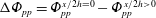 $\unicode[STIX]{x0394}\unicode[STIX]{x1D6F7}_{pp}=\unicode[STIX]{x1D6F7}_{pp}^{x/2h=0}-\unicode[STIX]{x1D6F7}_{pp}^{x/2h>0}$
, i.e. the difference of the
$\unicode[STIX]{x0394}\unicode[STIX]{x1D6F7}_{pp}=\unicode[STIX]{x1D6F7}_{pp}^{x/2h=0}-\unicode[STIX]{x1D6F7}_{pp}^{x/2h>0}$
, i.e. the difference of the
 $\unicode[STIX]{x1D6F7}_{pp}$
between the root location
$\unicode[STIX]{x1D6F7}_{pp}$
between the root location
 $x/2h=0$
and
$x/2h=0$
and
 $x/2h=0.5$
(green) and
$x/2h=0.5$
(green) and
 $1$
(blue). The continuous and dashed lines represent the serration and combed serration respectively.
$1$
(blue). The continuous and dashed lines represent the serration and combed serration respectively.
As previously discussed, the presence of the trailing-edge add ons alters the distribution and convection of the turbulent structures, thus affecting both the spanwise correlation length
 $l_{z}$
and the convective velocity
$l_{z}$
and the convective velocity
 $u_{c}$
of the surface pressure fluctuations, which are the most relevant parameters for TBL-TE noise prediction. In conventional trailing-edge noise theory, they are directly proportional to the noise radiation (Amiet Reference Amiet1976). Furthermore, as discussed in the Introduction, it was shown by Lyu et al. (Reference Lyu, Azarpeyvand and Sinayoko2016) that the spanwise correlation length is also related to noise decrease in presence of trailing-edge serrations. For this reason, the latter is estimated for all the configurations. The spanwise correlation length
$u_{c}$
of the surface pressure fluctuations, which are the most relevant parameters for TBL-TE noise prediction. In conventional trailing-edge noise theory, they are directly proportional to the noise radiation (Amiet Reference Amiet1976). Furthermore, as discussed in the Introduction, it was shown by Lyu et al. (Reference Lyu, Azarpeyvand and Sinayoko2016) that the spanwise correlation length is also related to noise decrease in presence of trailing-edge serrations. For this reason, the latter is estimated for all the configurations. The spanwise correlation length
 $l_{z}$
is defined as
$l_{z}$
is defined as
 $$\begin{eqnarray}\displaystyle l_{z}(x,f)=\int _{-\infty }^{\infty }\sqrt{\unicode[STIX]{x1D6FE}^{2}(x,\unicode[STIX]{x0394}z,f)}\,\text{d}z, & & \displaystyle\end{eqnarray}$$
where
 $\unicode[STIX]{x1D6FE}^{2}$
is the magnitude-squared coherence evaluated along the spanwise direction
$\unicode[STIX]{x1D6FE}^{2}$
is the magnitude-squared coherence evaluated along the spanwise direction
 $z$
.
$z$
.
 $\unicode[STIX]{x0394}z$
is the spanwise distance between the reference point and any other point along the span.
$\unicode[STIX]{x0394}z$
is the spanwise distance between the reference point and any other point along the span.
 $\unicode[STIX]{x1D6FE}^{2}$
is computed with a periodogram approach using a Hanning window and
$\unicode[STIX]{x1D6FE}^{2}$
is computed with a periodogram approach using a Hanning window and
 $50\,\%$
overlap. The resulting frequency resolution is equal to
$50\,\%$
overlap. The resulting frequency resolution is equal to
 $300$
Hz. In order to improve convergence, data are spatially averaged over all the serrations present in the computational domain, as previously discussed. Contour plots of
$300$
Hz. In order to improve convergence, data are spatially averaged over all the serrations present in the computational domain, as previously discussed. Contour plots of
 $\unicode[STIX]{x1D6FE}^{2}$
versus
$\unicode[STIX]{x1D6FE}^{2}$
versus
 $\unicode[STIX]{x0394}z/\unicode[STIX]{x1D6FF}$
and
$\unicode[STIX]{x0394}z/\unicode[STIX]{x1D6FF}$
and
 $St_{l}$
are plotted in figure 19, where
$St_{l}$
are plotted in figure 19, where
 $\unicode[STIX]{x1D6FF}$
is the boundary-layer thickness at
$\unicode[STIX]{x1D6FF}$
is the boundary-layer thickness at
 $x/l=-0.005$
(table 1). The reference point is chosen at the serration centreline
$x/l=-0.005$
(table 1). The reference point is chosen at the serration centreline
 $z/l=0$
. Figure 19 shows
$z/l=0$
. Figure 19 shows
 $\unicode[STIX]{x1D6FE}^{2}$
at three streamwise locations along the serrated surface (
$\unicode[STIX]{x1D6FE}^{2}$
at three streamwise locations along the serrated surface (
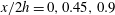 $x/2h=0,0.45,0.9$
) and at the location of the straight trailing edge for the baseline configuration (
$x/2h=0,0.45,0.9$
) and at the location of the straight trailing edge for the baseline configuration (
 $x/2h=0$
). It is visible that, as expected for turbulent flows,
$x/2h=0$
). It is visible that, as expected for turbulent flows,
 $\unicode[STIX]{x1D6FE}^{2}$
monotonically decreases with increasing
$\unicode[STIX]{x1D6FE}^{2}$
monotonically decreases with increasing
 $\unicode[STIX]{x0394}z$
. This is true regardless of the reference location. At the root location, both serrated trailing edges show larger magnitude with respect to the straight trailing edge for higher
$\unicode[STIX]{x0394}z$
. This is true regardless of the reference location. At the root location, both serrated trailing edges show larger magnitude with respect to the straight trailing edge for higher
 $\unicode[STIX]{x0394}z$
. Closer to the tip, the computation of
$\unicode[STIX]{x0394}z$
. Closer to the tip, the computation of
 $\unicode[STIX]{x1D6FE}^{2}$
is limited by the spanwise extent of the solid surface.
$\unicode[STIX]{x1D6FE}^{2}$
is limited by the spanwise extent of the solid surface.

Figure 19. Spanwise magnitude-squared coherence
 $\unicode[STIX]{x1D6FE}^{2}$
versus the chord-based Strouhal number
$\unicode[STIX]{x1D6FE}^{2}$
versus the chord-based Strouhal number
 $St_{l}$
. Each column represents a studied configuration: (a,d,f) sawtooth, (b,e,g) combed sawtooth, (c) straight. Each row reports a location in the streamwise direction: (a–c)
$St_{l}$
. Each column represents a studied configuration: (a,d,f) sawtooth, (b,e,g) combed sawtooth, (c) straight. Each row reports a location in the streamwise direction: (a–c)
 $x/2h=0$
, (d,e)
$x/2h=0$
, (d,e)
 $x/2h=0.45$
, (f,g)
$x/2h=0.45$
, (f,g)
 $x/2h=0.9$
.
$x/2h=0.9$
.

Figure 20. Spanwise correlation length (
 $l_{z}$
) versus the Strouhal number based on the chord (
$l_{z}$
) versus the Strouhal number based on the chord (
 $St_{l}$
). For the serrated configurations
$St_{l}$
). For the serrated configurations
 $l_{z}$
is averaged along the entire serration length.
$l_{z}$
is averaged along the entire serration length.
In order to easily compare both configurations, a simplification is carried out: the streamwise varying
 $l_{z}$
is averaged over the entire serration and plotted versus
$l_{z}$
is averaged over the entire serration and plotted versus
 $St_{l}$
in figure 20. This is done to retrieve a single frequency-dependent
$St_{l}$
in figure 20. This is done to retrieve a single frequency-dependent
 $l_{z}$
curve, which can be compared with the one of the straight trailing edge. For the straight trailing edge, data are averaged in the spanwise and not in the streamwise direction. This procedure results in a serration with a uniform distribution of
$l_{z}$
curve, which can be compared with the one of the straight trailing edge. For the straight trailing edge, data are averaged in the spanwise and not in the streamwise direction. This procedure results in a serration with a uniform distribution of
 $l_{z}$
on the entire surface. This approach is similar to the one adopted in analytical models for serrated trailing-edge noise (Lyu et al.
Reference Lyu, Azarpeyvand and Sinayoko2016). Within the limit of this simplification, the averaged spanwise correlation length
$l_{z}$
on the entire surface. This approach is similar to the one adopted in analytical models for serrated trailing-edge noise (Lyu et al.
Reference Lyu, Azarpeyvand and Sinayoko2016). Within the limit of this simplification, the averaged spanwise correlation length
 $l_{z}$
is larger for both the conventional and combed-sawtooth serrations with respect to the straight configuration. For all the configurations,
$l_{z}$
is larger for both the conventional and combed-sawtooth serrations with respect to the straight configuration. For all the configurations,
 $l_{z}$
decreases when increasing the frequency but with a different slope. In particular, it decreases faster for the serrated cases. The three curves collapse for
$l_{z}$
decreases when increasing the frequency but with a different slope. In particular, it decreases faster for the serrated cases. The three curves collapse for
 $St_{l}>20$
that corresponds to a wavelength based on the convective velocity (figure 21) approximately equal to
$St_{l}>20$
that corresponds to a wavelength based on the convective velocity (figure 21) approximately equal to
 $\unicode[STIX]{x1D6FF}$
. For
$\unicode[STIX]{x1D6FF}$
. For
 $St_{l}\approx 20$
,
$St_{l}\approx 20$
,
 $l_{z}\approx \unicode[STIX]{x1D6FF}^{\ast }$
, where
$l_{z}\approx \unicode[STIX]{x1D6FF}^{\ast }$
, where
 $\unicode[STIX]{x1D6FF}^{\ast }$
is the boundary-layer displacement thickness at
$\unicode[STIX]{x1D6FF}^{\ast }$
is the boundary-layer displacement thickness at
 $x/l=-0.005$
(table 1). This is in line with the observations of Jones & Sandberg (Reference Jones and Sandberg2012), where instead a split plate was used as baseline configuration, who stated that serrations would not alter the flow features for high non-dimensional frequencies. Linking these results with the instantaneous flow field (figures 13 and 14), it is possible to argue that the larger
$x/l=-0.005$
(table 1). This is in line with the observations of Jones & Sandberg (Reference Jones and Sandberg2012), where instead a split plate was used as baseline configuration, who stated that serrations would not alter the flow features for high non-dimensional frequencies. Linking these results with the instantaneous flow field (figures 13 and 14), it is possible to argue that the larger
 $l_{z}$
is caused by a milder interaction of the turbulent flow over the two sides of the aerofoil. For
$l_{z}$
is caused by a milder interaction of the turbulent flow over the two sides of the aerofoil. For
 $St_{l}<20$
, the filaments slightly reduce
$St_{l}<20$
, the filaments slightly reduce
 $l_{z}$
and no additional benefit is obtained by using combed-sawtooth serrations. It suggests that smaller structures are perturbed by the flow passing through the filaments. This could be responsible for the slight noise increase for
$l_{z}$
and no additional benefit is obtained by using combed-sawtooth serrations. It suggests that smaller structures are perturbed by the flow passing through the filaments. This could be responsible for the slight noise increase for
 $20<St_{l}<30$
.
$20<St_{l}<30$
.

Figure 21. Convective velocity of the surface pressure fluctuations
 $u_{c}$
versus the Strouhal number based on the chord
$u_{c}$
versus the Strouhal number based on the chord
 $St_{l}$
.
$St_{l}$
.
For a straight trailing edge, a larger
 $l_{z}$
results in higher far-field noise (Amiet Reference Amiet1976; Moreau & Roger Reference Moreau and Roger2009). The opposite trend is found for a slanted trailing edge. However, following the extension of Amiet’s theory for a serrated trailing edge formulated by Lyu et al. (Reference Lyu, Azarpeyvand and Sinayoko2016), for a given slanted edge and acoustic wavenumber, a larger
$l_{z}$
results in higher far-field noise (Amiet Reference Amiet1976; Moreau & Roger Reference Moreau and Roger2009). The opposite trend is found for a slanted trailing edge. However, following the extension of Amiet’s theory for a serrated trailing edge formulated by Lyu et al. (Reference Lyu, Azarpeyvand and Sinayoko2016), for a given slanted edge and acoustic wavenumber, a larger
 $l_{z}$
, which is uniform along the edge, would be beneficial for noise reduction since the effective correlated serration-averaged amplitude is
$l_{z}$
, which is uniform along the edge, would be beneficial for noise reduction since the effective correlated serration-averaged amplitude is
 $2h_{e}=l_{z}\unicode[STIX]{x1D70E}$
, where
$2h_{e}=l_{z}\unicode[STIX]{x1D70E}$
, where
 $\unicode[STIX]{x1D70E}=4h/\unicode[STIX]{x1D706}$
is the serration shape factor. The spatial average effect of the combed-sawtooth serrations is then to increase the spanwise correlation length of the coherent structure, which tend to aligned with the serration edge (Avallone et al.
Reference Avallone, Pröbsting and Ragni2016b
), thus promoting destructive interference (figure 11) between the scattered pressure waves within one correlation length. This finding supports the idea that a serration acts as a filter and that separate sub-critical and super-critical gust components (Graham Reference Graham1970). The efficiency of the separation is higher when the turbulent eddies are convected smoothly along the serration and their spanwise correlation length is much larger than the boundary-layer displacement thickness at the root. This finding also explains why analytical models do not predict any sound reduction or sound increase at high frequency. In the models of Howe (Reference Howe1991a
) and Lyu et al. (Reference Lyu, Azarpeyvand and Sinayoko2016), which are based on the spanwise correlation length model of Corcos (Reference Corcos1964), the effective correlated serration amplitude is only function of the shape factor and not of the frequency. Then, it is possible to argue that the frequency dependence and the faster decay rate of the spanwise correlation length is responsible for no noise reduction at high frequency.
$\unicode[STIX]{x1D70E}=4h/\unicode[STIX]{x1D706}$
is the serration shape factor. The spatial average effect of the combed-sawtooth serrations is then to increase the spanwise correlation length of the coherent structure, which tend to aligned with the serration edge (Avallone et al.
Reference Avallone, Pröbsting and Ragni2016b
), thus promoting destructive interference (figure 11) between the scattered pressure waves within one correlation length. This finding supports the idea that a serration acts as a filter and that separate sub-critical and super-critical gust components (Graham Reference Graham1970). The efficiency of the separation is higher when the turbulent eddies are convected smoothly along the serration and their spanwise correlation length is much larger than the boundary-layer displacement thickness at the root. This finding also explains why analytical models do not predict any sound reduction or sound increase at high frequency. In the models of Howe (Reference Howe1991a
) and Lyu et al. (Reference Lyu, Azarpeyvand and Sinayoko2016), which are based on the spanwise correlation length model of Corcos (Reference Corcos1964), the effective correlated serration amplitude is only function of the shape factor and not of the frequency. Then, it is possible to argue that the frequency dependence and the faster decay rate of the spanwise correlation length is responsible for no noise reduction at high frequency.
As discussed before in § 6, the boundary-layer thickness decreases from the root to the tip, thus accelerating the flow. This might induce an increase of the convective velocity
 $u_{c}$
, which affects the far-field noise. Since the far-field noise reduction is a function of frequency,
$u_{c}$
, which affects the far-field noise. Since the far-field noise reduction is a function of frequency,
 $u_{c}$
is computed for all the points along the edge following a spectral approach (Panton & Robert Reference Panton and Robert1994):
$u_{c}$
is computed for all the points along the edge following a spectral approach (Panton & Robert Reference Panton and Robert1994):
 $$\begin{eqnarray}\displaystyle u_{c}(x,z,f)=2\unicode[STIX]{x03C0}\unicode[STIX]{x0394}x\left(\frac{\unicode[STIX]{x2202}\unicode[STIX]{x1D719}}{\unicode[STIX]{x2202}f}\right)^{-1}, & & \displaystyle\end{eqnarray}$$
where
 $\unicode[STIX]{x1D719}$
is the phase obtained from the cross-spectral density between adjacent cells in the streamwise direction with distance
$\unicode[STIX]{x1D719}$
is the phase obtained from the cross-spectral density between adjacent cells in the streamwise direction with distance
 $\unicode[STIX]{x0394}x$
. In the following, results are averaged along the entire edge in order to easily compare the serrated case with the straight trailing edge (Kim et al.
Reference Kim, Haeri and Joseph2016) and plotted in figure 21. Although not shown here, it has been verified (van der Velden & Oerlemans Reference van der Velden and Oerlemans2017) that the frequency averaged convective velocity increases from the root to the tip of the serration as found experimentally (Arce-León et al.
Reference Arce-León, Merino-Martínez, Ragni, Avallone and Snellen2016b
; Avallone et al.
Reference Avallone, Pröbsting and Ragni2016b
). This causes a higher streamwise averaged
$\unicode[STIX]{x0394}x$
. In the following, results are averaged along the entire edge in order to easily compare the serrated case with the straight trailing edge (Kim et al.
Reference Kim, Haeri and Joseph2016) and plotted in figure 21. Although not shown here, it has been verified (van der Velden & Oerlemans Reference van der Velden and Oerlemans2017) that the frequency averaged convective velocity increases from the root to the tip of the serration as found experimentally (Arce-León et al.
Reference Arce-León, Merino-Martínez, Ragni, Avallone and Snellen2016b
; Avallone et al.
Reference Avallone, Pröbsting and Ragni2016b
). This causes a higher streamwise averaged
 $u_{c}$
with respect to the baseline configuration. As expected, for all the configurations under investigation,
$u_{c}$
with respect to the baseline configuration. As expected, for all the configurations under investigation,
 $u_{c}$
decreases with increasing
$u_{c}$
decreases with increasing
 $St_{l}$
since smaller eddies are convected closer to the wall. For the baseline configuration, at frequency
$St_{l}$
since smaller eddies are convected closer to the wall. For the baseline configuration, at frequency
 $St_{l}>20$
, a small increase is seen. Small differences are measured when comparing the two serrated geometries:
$St_{l}>20$
, a small increase is seen. Small differences are measured when comparing the two serrated geometries:
 $u_{c}$
is larger for the combed-sawtooth serrations for
$u_{c}$
is larger for the combed-sawtooth serrations for
 $St_{l}<13$
, while it is lower at higher frequencies. The larger
$St_{l}<13$
, while it is lower at higher frequencies. The larger
 $u_{c}$
might be caused by the more uniform flow over the serrations and the absence of strong discontinuities due to the wake flow between teeth. The larger
$u_{c}$
might be caused by the more uniform flow over the serrations and the absence of strong discontinuities due to the wake flow between teeth. The larger
 $u_{c}$
for the serrated trailing edges might cause higher noise with respect to the straight trailing edge.
$u_{c}$
for the serrated trailing edges might cause higher noise with respect to the straight trailing edge.
To better compare the combined effect of
 $l_{z}$
and
$l_{z}$
and
 $u_{c}$
, their product is plotted in figure 22. The figure clearly shows trends close to the one obtained when comparing far-field noise (figure 7). No difference between the three configurations is present for
$u_{c}$
, their product is plotted in figure 22. The figure clearly shows trends close to the one obtained when comparing far-field noise (figure 7). No difference between the three configurations is present for
 $St_{l}>20$
. This plot and the ones discussed above suggest that the most relevant hydrodynamic parameter that controls noise reduction is the spanwise correlation length of the surface pressure fluctuations
$St_{l}>20$
. This plot and the ones discussed above suggest that the most relevant hydrodynamic parameter that controls noise reduction is the spanwise correlation length of the surface pressure fluctuations
 $l_{z}$
, which leads to destructive interference. However, this effect is modulated by the larger convective velocity that increases the intensity of the scattered pressure waves.
$l_{z}$
, which leads to destructive interference. However, this effect is modulated by the larger convective velocity that increases the intensity of the scattered pressure waves.
8 Conclusions
The turbulent flow over a NACA 0018 aerofoil with and without trailing-edge serrations and the resulting scattered turbulent boundary-layer trailing-edge noise were studied to investigate the physical noise reduction mechanisms. The flow field was computed by solving the explicit, transient, compressible lattice Boltzmann equations, while the acoustic far field was obtained by means of the Ffowcs Williams and Hawkings integral solution. Both conventional sawtooth and combed-sawtooth trailing-edge add ons were compared with the straight trailing-edge configuration. Boundary-layer transition was forced by means of a zig–zag strip along both sides of the aerofoil. A grid resolution study and comparison against experimental data was used to assess the computational set-up. Computational results agree with previous experimental PIV and acoustic beamforming results (Arce-León et al. Reference Arce-León, Merino-Martínez, Ragni, Avallone and Snellen2016b ; Avallone et al. Reference Avallone, Pröbsting and Ragni2016b ).

Figure 22. Product of the convective velocity (
 $u_{c}$
) and spanwise correlation length (
$u_{c}$
) and spanwise correlation length (
 $l_{z}$
) versus the Strouhal number based on the chord (
$l_{z}$
) versus the Strouhal number based on the chord (
 $St_{l}$
).
$St_{l}$
).
Noise reduction depends on the frequency. Sawtooth serrations show approximately 6 dB noise reduction with respect to the straight configuration. Combed-sawtooth serrations attain additional 3 dB noise reduction than the conventional sawtooth serrations at the same non-dimensional frequency. The additional noise reduction is in agreement with in-field measurements (Oerlemans Reference Oerlemans2016). For both configurations, the maximum noise reduction is obtained for
 $St_{l}$
approximately equal to
$St_{l}$
approximately equal to
 $8$
. This represents the non-dimensional frequency corresponding of the most amplified flow instability (Jones et al.
Reference Jones, Sandberg and Sandham2009). Trailing-edge serrations reduce noise for
$8$
. This represents the non-dimensional frequency corresponding of the most amplified flow instability (Jones et al.
Reference Jones, Sandberg and Sandham2009). Trailing-edge serrations reduce noise for
 $St_{l}<30$
while at higher frequencies no noise reduction is found in agreement with Jones & Sandberg (Reference Jones and Sandberg2012). For a given serration geometry, the introduction of filaments in the empty space between teeth does not affect the frequency range over which serrations reduce noise but only the maximum noise reduction.
$St_{l}<30$
while at higher frequencies no noise reduction is found in agreement with Jones & Sandberg (Reference Jones and Sandberg2012). For a given serration geometry, the introduction of filaments in the empty space between teeth does not affect the frequency range over which serrations reduce noise but only the maximum noise reduction.
The serrated surface was split into strips to study the constructive/destructive interference between scattered acoustic pressure waves along the edge. Results and their comparison with dilatation field plots suggest that the main effect of trailing-edge serrations, with and without filaments, is to create destructive interference between pressure waves scattered along the edge. Interference between strips depends on the frequency. The results further confirm previous experimental assumptions that most of the noise is generated at the root of the serrations (Avallone et al. Reference Avallone, Pröbsting and Ragni2016b ). The presence of the combs mitigates this effect at the root, spreading more uniformly the noise sources along the entire serrations.
Aiming at detecting the physical parameters that contribute to noise mitigation, the instantaneous and time-averaged flow fields were analysed. They show that the introduction of sawtooth serrations promotes the formation of elongated coherent structures in the wake in the empty space between serrations together with hairpin vortices along the sawtooth edges. The introduction of slits mitigates the interaction between the two sides of the serrations and avoids the formation of the wake. Direct consequence is a more uniform distribution of the coherent flow structures. The effect of such modification on the time-averaged flow field is to mitigate the both the outward (i.e. from the centreline toward the edge) and inward (i.e. from the edge toward the centreline) flow motions.
Differences in the instantaneous flow organization leads to a different statistical characterization of the surface pressure fluctuations. For this reason, the spanwise correlation length
 $l_{z}$
and the convective velocity
$l_{z}$
and the convective velocity
 $u_{c}$
of the surface pressure fluctuations were investigated, since related to noise generation. It is found that
$u_{c}$
of the surface pressure fluctuations were investigated, since related to noise generation. It is found that
 $l_{z}$
varies in the streamwise direction. The streamwise averaged
$l_{z}$
varies in the streamwise direction. The streamwise averaged
 $l_{z}$
increases in presence of trailing-edge serrations for
$l_{z}$
increases in presence of trailing-edge serrations for
 $St_{l}<20$
. It increases more in presence of combed-sawtooth serrations. This integral correlation length tends to the value of the straight trailing edge for
$St_{l}<20$
. It increases more in presence of combed-sawtooth serrations. This integral correlation length tends to the value of the straight trailing edge for
 $St_{l}>20$
. This is due to the milder spanwise flow discontinuity imposed by the installation of the slits. Following Lyu et al. (Reference Lyu, Azarpeyvand and Sinayoko2016), larger
$St_{l}>20$
. This is due to the milder spanwise flow discontinuity imposed by the installation of the slits. Following Lyu et al. (Reference Lyu, Azarpeyvand and Sinayoko2016), larger
 $l_{z}$
might be beneficial to noise reduction by promoting destructive interference because of the phase difference between scattered pressure waves. When
$l_{z}$
might be beneficial to noise reduction by promoting destructive interference because of the phase difference between scattered pressure waves. When
 $l_{z}$
is closer to the one obtained in presence of a straight trailing edge no additional benefit in terms of noise reduction is found, thus suggesting that the flow no longer sees the slanted edge. Similarly,
$l_{z}$
is closer to the one obtained in presence of a straight trailing edge no additional benefit in terms of noise reduction is found, thus suggesting that the flow no longer sees the slanted edge. Similarly,
 $u_{c}$
increases in presence of serrated edges. The introduction of filaments further increases
$u_{c}$
increases in presence of serrated edges. The introduction of filaments further increases
 $u_{c}$
for
$u_{c}$
for
 $St_{l}<20$
with respect to the conventional sawtooth trailing edge. Differently,
$St_{l}<20$
with respect to the conventional sawtooth trailing edge. Differently,
 $u_{c}$
decreases for
$u_{c}$
decreases for
 $St_{l}>20$
. Also this effect is attributed to the milder spanwise discontinuity and the thinner boundary layer on the serration surface. The product of the two quantities averaged along the entire surface shows trends similar to the far-field noise curve.
$St_{l}>20$
. Also this effect is attributed to the milder spanwise discontinuity and the thinner boundary layer on the serration surface. The product of the two quantities averaged along the entire surface shows trends similar to the far-field noise curve.
It is possible to conclude that trailing-edge serrations reduce noise because of destructive interference between radiated acoustic pressure waves for which a larger spanwise correlation length is beneficial. The disagreement between literature and measurements is caused by the different decay rate of the spanwise correlation length with respect to the one for a straight trailing edge, thus affecting the effective correlated length of serrations, which become frequency dependent. The computed
 $l_{z}$
and
$l_{z}$
and
 $u_{c}$
might be used as input in the analytical model to verify that it can improve far-field noise prediction for serrated trailing edges.
$u_{c}$
might be used as input in the analytical model to verify that it can improve far-field noise prediction for serrated trailing edges.
Acknowledgements
The research of Dr W.C.P. van der Velden during his PhD was funded and supported by Siemens Wind Power A/S, Brande, Denmark.
Appendix. Experimental set-up
The reference experiments from Arce-León et al. (Reference Arce-León, Merino-Martínez, Ragni, Avallone and Snellen2016b
) were conducted at the Delft University of Technology vertical wind tunnel (V-Tunnel). It has a contraction ratio of approximately
 $60:1$
. For these measurements a square nozzle of
$60:1$
. For these measurements a square nozzle of
 $40\times 40~\text{cm}^{2}$
was used. The turbulence intensity was below
$40\times 40~\text{cm}^{2}$
was used. The turbulence intensity was below
 $0.5\,\%$
for the range of tested velocities.
$0.5\,\%$
for the range of tested velocities.
A NACA 0018 aerofoil with chord of 20 cm and span of 40 cm was installed in the V-Tunnel between two 1.5 m long side plates to approximate the two-dimensional flow condition over most of the wing. The aerofoil leading edge was located at 0.5 m from the contraction exit. A modular trailing edge allowed inserts (i.e. the straight and the sawtooth trailing-edge serrations) to be retrofitted while keeping the surface free from irregularities. The geometry of the trailing edge serrations was the same of the one of the current manuscript.
Boundary-layer transition was forced to turbulent with randomly distributed roughness elements. The trip tape was constructed by a random distribution of carborundum elements with nominal size of 0.6 mm, placed on a thin double side tape of 1 cm width. The tape was streamwise centred at
 $20\,\%$
of the chord and was applied for the entire aerofoil span. A stethoscope probe was used to verify that the boundary layer was turbulent until the trailing edge.
$20\,\%$
of the chord and was applied for the entire aerofoil span. A stethoscope probe was used to verify that the boundary layer was turbulent until the trailing edge.
Particle image velocimetry data were obtained with high-speed stereoscopic-PIV set-up at three streamwise aligned planes located at
 $z/\unicode[STIX]{x1D706}=0,0.25$
and
$z/\unicode[STIX]{x1D706}=0,0.25$
and
 $0.5$
. The data used as comparison in this manuscript were obtained from an uncorrelated data set of 2000 particle images acquired at a frequency of 250 Hz for 8 s.
$0.5$
. The data used as comparison in this manuscript were obtained from an uncorrelated data set of 2000 particle images acquired at a frequency of 250 Hz for 8 s.
Acoustic data were obtained using an array of
 $64$
microphones and an effective diameter of 0.9 m. Microphones were arranged in a multi-arm spiral configuration. The chosen configuration resulted in a minimum resolvable distance of 12 mm. Acoustic data were acquired at a sampling frequency of 50 kHz for 60 s. To isolate trailing-edge noise, beamforming data were integrated over an area extending between
$64$
microphones and an effective diameter of 0.9 m. Microphones were arranged in a multi-arm spiral configuration. The chosen configuration resulted in a minimum resolvable distance of 12 mm. Acoustic data were acquired at a sampling frequency of 50 kHz for 60 s. To isolate trailing-edge noise, beamforming data were integrated over an area extending between
 $z=-10~\text{cm}$
and
$z=-10~\text{cm}$
and
 $z=0.1~\text{cm}$
and
$z=0.1~\text{cm}$
and
 $x=-6~\text{mm}$
and
$x=-6~\text{mm}$
and
 $x=6~\text{mm}$
.
$x=6~\text{mm}$
.


 Open access