


1. INTRODUCTION
Contemporary glacial retreat is widely regarded as evidence of anthropogenic climate change (Vaughan and others, Reference Vaughan2013; Zemp and others, Reference Zemp2015; Roe and others, Reference Roe, Baker and Herla2017) and geologic records of past glacial extents are utilized as archives of past climate changes (Porter, Reference Porter1975; Lowell, Reference Lowell2000; Anderson and Mackintosh, Reference Anderson and Mackintosh2006; Doughty and others, Reference Doughty2013). Local meteorology and glacier geometry dictate surface mass balance, and surface mass balance and mass transport within the glacier determine the length (Oerlemans, Reference Oerlemans2001; Cuffey and Paterson, Reference Cuffey and Paterson2010). Long-term changes in local meteorology (i.e., climate change) thus reflect themselves in glacier-length changes, providing a potentially useful climate proxy in the absence of direct measurements of climatic variables.
Snow and ice accumulation and the surface energy balance dictate mass balance (Oerlemans, Reference Oerlemans2001; Cuffey and Paterson, Reference Cuffey and Paterson2010), but changes in glacier length can often be modeled using only two key climate variables: air-temperature and precipitation (Oerlemans, Reference Oerlemans2005; Leclercq and Oerlemans, Reference Leclercq and Oerlemans2012). The importance of these two climate variables relative to each other largely depends on a glacier's climate setting, with wetter glaciers being more sensitive to temperature and drier glaciers being more sensitive to precipitation (Oerlemans and Fortuin, Reference Oerlemans and Fortuin1992; Rupper and Roe, Reference Rupper and Roe2008). Seasonality in these two variables can also play a role (Oerlemans and Reichert, Reference Oerlemans and Reichert2000; Fujita, Reference Fujita2008a,Reference Fujitab). Accounting for possible seasonality changes in analyses can affect the climatological interpretations of past glacier-length changes (Vacco and others, Reference Vacco, Alley and Pollard2009). Thus, records and observations of glacier-length changes are often used to infer past and ongoing climate changes.
Glacier-length fluctuations, however, can also occur in an unchanging climate, complicating climatological interpretations of glacier-length changes. Model results suggest that mass-balance anomalies associated with year-to-year variations in air-temperature and precipitation (i.e., interannual climate variability) can drive glacier-length fluctuations independent of changes in the mean climate (Oerlemans, Reference Oerlemans2000; Roe and O'Neal, Reference Roe and O'Neal2009; Huybers and Roe, Reference Huybers and Roe2009; Roe and Baker, Reference Roe and Baker2014). Thus, climatological interpretations of glacier-length changes are a statistical exercise of disentangling the portion that could be caused by length fluctuations due to interannual climate variability from the portion that requires a change in the average glacier length (Roe, Reference Roe2011; Anderson and others, Reference Anderson, Roe and Anderson2014; Roe and others, Reference Roe, Baker and Herla2017; Herla and others, Reference Herla, Roe and Marzeion2017). Changes in average glacier length, however, are usually associated with changes in the mean climate, but a portion of average length changes could also be due to changes in interannual climate variability. Farinotti (Reference Farinotti2013) and Malone and others (Reference Malone, Pierrehumbert, Lowell, Kelly and Stroup2015), using different numerical modeling techniques, find that the mean length of a glacier retreats upslope as the magnitude of interannual climate variability increases. Thus, the role of interannual climate variability on the average length and mass balance of glaciers warrants further investigation.
The aim of this study is to quantify the effects of interannual climate variability (henceforth referred to as just interannual variability) on the average length and mass balance of glaciers (i.e., their mean state). Changes in average glacier length and mass balance due to changes in interannual variability are quantified using idealized numerical modeling. Studies are conducted for glaciers in three different climate settings, spanning several different types of glaciers. For all three glaciers, the mean state is partially determined by the magnitude of interannual variability, due to a mass-balance asymmetry between warm and cold years. This asymmetry is identified and its presence in observational and modeling studies is discussed. The ability to detect mass-balance asymmetries in the glaciological record is evaluated, and the impact of this mass-balance asymmetry on paleoclimate reconstructions is discussed.
2. METHODS
To simulate the transient and average glacier-length response to interannual variability, a shallow ice 1-D flowline model is coupled to a simplified model for surface mass balance. Similar approaches have been used to simulate glacier-length response to climate change and interannual variability (Oerlemans and others, Reference Oerlemans1998; Oerlemans, Reference Oerlemans2000; Anderson and Mackintosh, Reference Anderson and Mackintosh2006; Roe and O'Neal, Reference Roe and O'Neal2009). Each model and the experiments conducted are described below.
2.1. Flowline model
Ice dynamics are simulated using a 1-D shallow-ice flowline model, which has been shown to capture ice deformation and sliding behavior of mountain glaciers (Oerlemans, Reference Oerlemans1986). The model requires two inputs: (1) topographic information about the valley and (2) surface mass balance. For topography, an idealized valley geometry is used with a constant bedrock slope (results are shown here for a 10° slope) and constant valley width. Surface mass balance is calculated using a simplified mass-balance model (see Section 2.2).
The governing equation for the 1-D flowline model is mass continuity for a constant density fluid constrained to a constant width:
 $$\displaystyle{{\partial H} \over {\partial t}} = -\displaystyle{\partial \over {\partial {\mkern 1mu} x}}(u{\mkern 1mu} H) + b$$
where H is the thickness of the glacier at a given point along the flowline, x, h is the height of the glacier surface above a datum, t is time, b is the surface mass balance, and u is the sum of the deformation velocity (u d) and sliding velocity (u s) at the point. Velocity relationships follow the form from Oerlemans (Reference Oerlemans1997):
 $$\eqalign{& u_{\rm d} = f_{\rm d}{\mkern 1mu} H{\mkern 1mu} \tau ^3 \cr & u_{\rm s} = f_{\rm s}{\mkern 1mu} H^{-1}{\mkern 1mu} \tau ^3} $$
where f d and f s are the parameters for deformation and sliding, respectively, τ is the driving stress (ρ g H (∂h/∂x)), g is the acceleration due to gravity, ρ is the ice density, and ∂ H/∂ x is the slope of the glacier surface. Equation (1) is solved using the Crank-Nicholson method with a time step of 1/500th of a year and a horizontal resolution of 25 m.
2.2. Mass-balance model
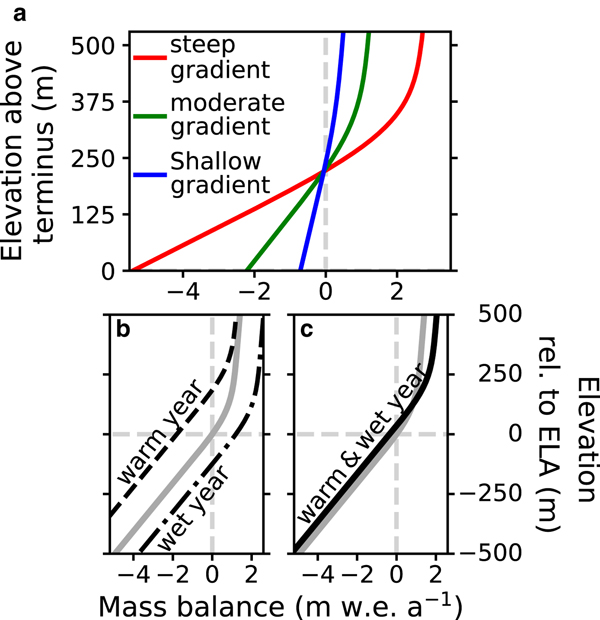
A mass-balance profile, which accounts for the variations in ablation/accumulation with elevation (Fig. 1a), is used for the surface mass-balance input into the flowline model. The change in the amount of surface mass loss/gain with elevation is referred to as the mass-balance gradient. For many glaciers, the mass-balance gradient is larger at lower elevations and smaller at higher elevations (Rea, Reference Rea2009; Benn and Evans, Reference Benn and Evans2014). The magnitude of the mass-balance gradient, particularly at lower elevations, also reflects the climate setting. Glaciers in warm maritime or tropical climates have some of the largest mass-balance gradients in their ablation zones (Kaser and Osmaston, Reference Kaser and Osmaston2002). Glaciers in mid-latitude continental climates have smaller mass-balance gradients, and glaciers in arid regions have the smallest gradients (Haefeli, Reference Haefeli1962; Kuhn, Reference Kuhn1981; Oerlemans, Reference Oerlemans2001; Kaser, Reference Kaser2001). Experiments are conducted for these three end-member climate settings, as represented by different mass-balance profiles (Fig. 1a). The three mass-balance profiles are differentiated henceforth by the steepness of the mass-balance gradient in their ablation zone as follows: (1) steep gradient (2.5 m w.e. a−1 100 m−1 ),(2) moderate (1.0 m w.e. a−1 100 m−1 ) gradient, (3) shallow gradient (0.3 m w.e. a−1 100 m−1 ) (values from Haefeli (Reference Haefeli1962); Kuhn (Reference Kuhn1981); Kaser and Osmaston (Reference Kaser and Osmaston2002)). For all three profiles, the mass-balance gradient at higher elevations is smaller, being only 0.1 m w.e. a−1 100 m−1 . This smaller mass-balance gradient is due to different surface mass-balance processes at higher elevations than at lower elevations. Its value largely depends on orographic precipitation and partitioning between rain and snow (Kuhn, Reference Kuhn1981; Oerlemans and Hoogendoorn, Reference Oerlemans and Hoogendoorn1989; Kaser, Reference Kaser2001).

Fig. 1. (a) Mass-balance profiles representative of glaciers in maritime or tropical (steep), mid-latitude continental glacier (moderate), and cold and arid (shallow) regions, (b) mass-balance profile response to a warm year (vertical translation) and wet year (horizontal translation), and (c) mass-balance profile response to a warm and wet year (superposition of the two translations in (b)). The two gradients transition smoothly 100 m above the equilibrium line altitude (ELA).
The mass-balance response to interannual variability is simulated by perturbing the mass-balance profile. The shape of a glacier's mass-balance profile remains approximately constant from year-to-year, but the intercept changes due to interannual variability (Meier and Tangborn, Reference Meier and Tangborn1965; Kaser and others, Reference Kaser2003). The size of the change reflects the magnitude of the interannual anomalies and the equilibrium line altitude (ELA) sensitivity. In this study, only air-temperature and precipitation anomalies are explored. The mass-balance response to air-temperature anomalies is simulated by vertical shifts in the mass-balance profiles (Fig. 1b). This method has been used to forecast the length evolution of Zongo Glacier (Bolivia) through the 21st century (Réveillet and others, Reference Réveillet, Rabatel, Gillet-Chaulet and Soruco2015). The mass-balance response to precipitation anomalies is simulated by horizontal shifts in the mass-balance profiles (Fig. 1b). This method assumes that anomalous precipitation is added equally to all elevations, which is consistent with previous studies on glacier-length responses to interannual variability Roe and O'Neal (Reference Roe and O'Neal2009); Huybers and Roe (Reference Huybers and Roe2009); Roe and Baker (Reference Roe and Baker2014)). In total, the mass-balance response to anomalies in air-temperature and precipitation is the superposition of the vertical and horizontal shifts (Fig. 1c).
The magnitude of the mass-balance profile translations defined above partially determines the size of the glacier-wide mass-balance anomaly. The magnitude of the vertical translation is equal to the product of the air-temperature anomaly and the ELA sensitivity to temperature. Réveillet and others (Reference Réveillet, Rabatel, Gillet-Chaulet and Soruco2015), who apply this vertical translation method to Zongo Glacier (Bolivia), use an observationally derived ELA sensitivity to temperature of 150±30 m °C−1;. In this study, the ELA sensitivity to temperature is assumed to be the inverse of the lapse rate, which is consistent with Sagredo and others (Reference Sagredo, Rupper and Lowell2014) for how ELA sensitivity to temperature varies regionally. A lapse rate of 6.5°C km−1 is used for all simulations, producing an ELA sensitivity to temperature of ~150 m °C−1;. The magnitude of the horizontal translation is equal to the amount of anomalous precipitation. The surface mass-balance response to interannual variability is simulated by perturbing the mass-balance profiles as described above.
2.3. Experiments: glacier-length response to interannual variability
The transient and average glacier-length response to interannual variability is simulated for each of the three end-member climate settings. To initialize each experiment, the flowline mode is run to equilibrium with each of the three representative mass-balance profiles. In equilibrium, the initialized glaciers are 3 km long. To ensure that each glacier is 3 km long, the ELA is moved vertically. The ELA is closest to the terminus for the glacier with the steepest mass-balance gradient and closest to the summit for the glacier with the shallowest mass-balance gradient. The mass loss at the terminus, however, is largest for the glacier with the steep mass-balance gradient and smallest for glacier with the shallow mass-balance gradient. Using the glacier response time formula from Roe and O'Neal (Reference Roe and O'Neal2009), the response times for the three different mass-balance profiles are: steep, τ = 12 years; moderate, τ = 22 years; and shallow, τ = 48 years. Once the initialization is complete, the mass-balance profiles are perturbed by adding interannual variability into the simulations. The resulting transient simulations are run for 10,100 model years. Analyses are conducted on the final 10,000 years of model output.
The mass-balance profiles are perturbed by interannual air-temperature and precipitation anomalies that are drawn randomly from Gaussian distributions with a prescribed standard deviation (1 − σ value). The two climate anomalies are uncorrelated in time from each other. For each model year, the mass-balance profile is perturbed by that year's air-temperature anomaly and precipitation anomaly, as described in Section 2.2. The timing of air-temperature and precipitation anomalies are the same for all simulations, and different magnitudes of variability are simulated by changing the amplitude of the anomalies. Simulations are conducted with precipitation anomalies with a 1 − σ value of 0.50 m w.e. a−1 and air-temperature anomalies with 1 − σ values ranging from 0.00 to 1.50°C, in increments of 0.25°C (n=7). Additionally, simulations are conducted without precipitation anomalies but air-temperature anomalies with 1 − σ value of 0.50°C (n=1). In total, eight transient simulations are conducted for each of the three climate settings (as simulated by the steep, moderate, and shallow mass-balance profiles).
In addition to the effects of interannual variability on the transient and average glacier length, the equilibrium response to a sustained change in the mass-balance profile is quantified. After the model spin-up is complete, the mass-balance profile is instantaneously changed to a new mass-balance profile and then run to equilibrium. The changes to the mass-balance profiles for these equilibrium simulations are discussed in Section 3.1. These equilibrium experiments help isolate the processes linking interannual variability to changes in the mean state.
3. RESULTS
3.1. Interannual variability and the mean state of glaciers
Interannual variability produces model glacier-length fluctuations around an average length, while also reducing the average length as compared to the spin-up model length without interannual variability (Fig. 2a). For the same timing and magnitude of interannual variability, the magnitude of the transient fluctuations differs (Fig. 2a). The shallow mass-balance gradient glacier has the largest magnitude of length fluctuations, and the moderate mass-balance gradient glacier has the smallest magnitude of length fluctuations (as quantified by the standard deviation of the glacier length time series, σ L). For the shallow, moderate and steep mass-balance gradient glaciers, the length variabilities are: σ L = 206, 126 and 131 m. The differences in size and timing of length fluctuations for identical interannual variability stems from two key differences between the glaciers: (1) response time (see Section 2.3 for values) and (2) magnitude of mass-balance variability. Details regarding how these differences can affect the size and timing of transient length fluctuations can be found in Roe and Baker (Reference Roe and Baker2014); Roe and others (Reference Roe, Baker and Herla2017); Mackintosh and others (Reference Mackintosh, Anderson and Pierrehumbert2017).
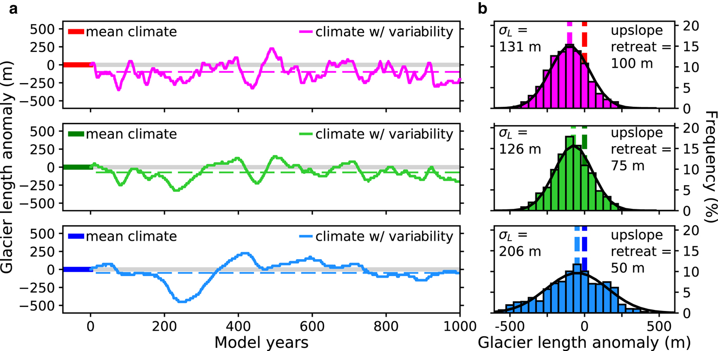
Fig. 2. (a) Glacier-length fluctuations due to interannual variability for the steep mass-balance gradient glacier (top), moderate mass-balance gradient glacier (middle), and shallow mass-balance gradient glacier (bottom) and (b) distribution of glacier-length fluctuations for the transient simulations, including normal distributions (black lines) with the same magnitude of length fluctuations. Length anomalies are relative to the 3-km spin-up length. Dashed lines represent the average glacier lengths in (a) and the equilibrium glacier length for the spin-up mass-balance profile (mean climate) and the time-averaged mass-balance profile (mean of climate w/ variability) in (b). All three glaciers are forced by the same timing of interannual variability. Only the first 1000 years of the 10,100-year transient simulations are shown in (a), and the final 10000 years of the transient simulations are used for the histograms and statistics in (b). Results are shown for interannual temperature variability with a 1 − σ value of 0.5°C and interannual precipitation variability with a 1 − σ value of 0.5 m w.e. a−1.
The average length around which these glaciers fluctuate, however, is shorter than the 3 km spin-up length (Table 1). During the first few decades to centuries of the transient simulations, all three glaciers fluctuate on top of a trend of upslope-retreat, with differing retreat rates (Fig. 2a). The steep mass-balance gradient glacier retreats the most (100 m), followed by the moderate mass-balance gradient glacier (75 m), and the shallow mass-balance gradient glacier retreats the least (50 m), for simulations with 25 m spatial resolution. After the glaciers reach their new average length, they fluctuate around this length for the remainder of the transient simulations.
Table 1. Transient and average glacier-length response to air-temperature and/or precipitation interannual variability: σ T = 0.5°C and/or σ P = 0.5 m w.e a−1

σ L is the standard deviation of the glacier length time series and the upslope retreat is how much shorter the average glacier length is compared to the 3 km spin-up length.
The average length of all three glaciers is partially determined by interannual climate variability, suggesting that the average mass balance also depends on interannual variability. For each climate setting, the time-average (mean) of the mass-balance profiles for the transient simulations has a different shape than the mass-balance profile for the mean climate (i.e., the climate without interannual variability). For the 3 km spin-up glacier length, these time-averaged mass-balance profiles produce negative glacier-wide mass balances; thus driving upslope retreat. To evaluate the role of this change in the mass-balance profile on the average glacier lengths, equilibrium glacier length simulations are conducted using the time-averaged mass-balance profiles as inputs to the flowline model. The equilibrium glacier lengths with the time-averaged mass-balance profiles are the same as the average glacier length from the transient simulations (Fig. 2b), within the model resolution (25 m). Both the average glacier length and the average mass-balance profile are at least partially determined by interannual climate variability, and it is the change in the average mass-balance profile that drives the change in the average glacier length.
3.2. Relationships between interannual variability and changes in the mean state
The transient and average response to interannual variability differs depending on whether forced by air-temperature or precipitation interannual variability (Table 1). Consistent with previous studies Roe and O'Neal (Reference Roe and O'Neal2009), the magnitude of glacier-length fluctuations from both air-temperature and precipitation variability (σ L) is roughly the linear combination of length fluctuations from air-temperature variability (σ L, T) and precipitation variability (σ L, P) (i.e.,  $\sigma _{L} = \sqrt { \sigma _{L,\, T}^{2} + \sigma _{L,\, P}^{2}}$). For the glacier with the steep mass-balance gradient, 86% of the standard deviation in glacier length fluctuations is driven by air-temperature variability. For the glacier with the shallow mass-balance gradient, 90% is driven by precipitation variability. For the glacier with the moderate mass-balance gradient, the transient length fluctuations are more evenly partitioned (temperature: 52%, precipitation: 48%). An upslope retreat, and thus a change in the mean state, only occurs when interannual air-temperature variability is included. The size of this retreat is identical to the size when forced with both air-temperature and precipitation variability. Interannual precipitation variability alone does not change the average glacier length. While the transient glacier length fluctuations can be driven by both air-temperature and precipitation interannual variability, we conclude that, to within the spatial resolution of the model (25 m), changes in the mean state are driven only by interannual air-temperature variability.
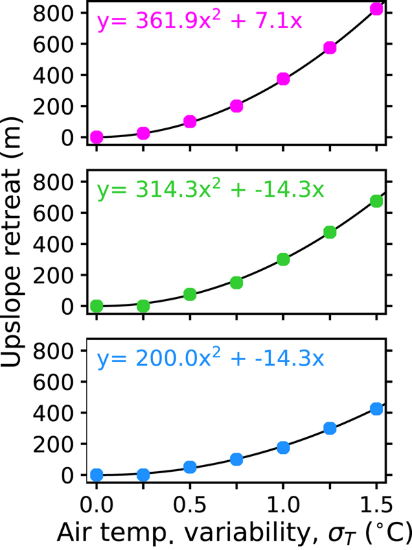
The size of the upslope retreat increases quadratically with increased interannual air-temperature variability (Fig. 3). The average length of the steep mass-balance gradient glacier retreats 100 m if the magnitude of the interannual temperature variability (quantified by a 1 − σ value) increases from 0.5 to 0.75°C. For this same glacier starting in a noisier climate, an increase in the interannual temperature variability from 1.0 to 1.25°C causes a 200 m retreat. For the shallow mass-balance gradient glacier, the same quadratic relationship holds, but the size of retreat is less. For the two scenarios given above, the retreat is 50 and 125 m. The moderate mass-balance glacier falls between these two extremes but closer to the steep mass-balance gradient limit. Three key factors affect how the mean state of a glacier responds to changes in interannual air-temperature variability: (1) climate setting of a glacier, (2) how noisy the interannual air-temperature variability is before the change in its magnitude and (3) the size of the change in interannual air-temperature variability. Changes in the mean glacier state due to changes in interannual variability are most acute for large changes in air-temperature variability at glaciers with steep mass-balance gradients that are found in climates with large interannual air-temperature variability.

Fig. 3. Upslope retreat due to the addition of different magnitudes of interannual temperature variability for the steep mass-balance gradient glacier (top), moderate mass-balance gradient glacier (middle) and shallow mass-balance gradient glacier (bottom). Quadratic models relating upslope retreat and the magnitude of interannual variability are included.
4. DISCUSSION
4.1. A mechanism for upslope retreat: mass-balance asymmetries
The results from the idealized modeling presented here suggest that interannual air-temperature variability partially defines the mean state of a glacier. Interannual air-temperature variability affects the mean state through a mass-balance asymmetry between warm and cold years: more mass is lost on a warm year than gained on a cold year of equal magnitude. Near the transition in mass-balance gradients (100 m above the ELA), a warm year produces a larger negative mass-balance perturbation than a positive perturbation during a cold year (Fig. 4). This mass-balance mismatch between warm and cold years near the point-of-inflection in the mass-balance profile produces an asymmetry that grows linearly as air-temperature variability increases (Fig. 4). At the same time, the area over which this asymmetry occurs increases as air-temperature variability increases. The area increases linearly with increasing air-temperature variability because of the method implemented for perturbing the mass-balance profiles and the constant width valley geometry (Section 2.2). The resulting asymmetry scales with the product of these two processes, producing a quadratic mass-balance asymmetry with increasing air-temperature variability. The quadratic mass-balance asymmetry is evident in the form of the upslope retreat of the glacier (Fig. 3).

Fig. 4. Mass-balance response to different signs and magnitudes of air temperature anomalies. The vertical displacements in the profile are symmetric to warm and cold anomalies, as prescribed by the methods, but the glacier-wide mass-balance response is asymmetric.
This asymmetry is the logical conclusion of a non-linear mass-balance profile that responds linearly to air-temperature perturbations. A linear mass-balance profile would not produce a mass-balance asymmetry and would not affect the mean state (Appendix). The size of the asymmetry increases as the difference in the mass-balance gradients between the upper and lower elevations (i.e., the amount of curvature in the mass-balance profile) increases and the amount of interannual air-temperature variability increases (Fig. 4). Additionally, the elevation range over which mass-balance gradients transition affects the asymmetry. The smaller the elevation range, the larger the curvature and the greater the asymmetry. Interannual precipitation variability does not influence the mean state since in this study accumulation anomalies respond symmetrically to precipitation perturbations.
Surface mass-balance asymmetries from short-term climate variability are noted in both observational and modeling studies. Bradley and England (Reference Bradley and England1978) illustrate that the long-term mass balance of the Devon Ice Cap (Canada) can be strongly influenced by one or a few warm years. The asymmetry in their study is a curvilinear relationship between mass balance and temperature -- negative mass-balance anomalies can grow almost limitlessly as hotter years produce more melt but there is a limit to positive mass-balance anomalies on colder years. Farinotti (Reference Farinotti2013) illustrates that increased temperature variability (at timescales from daily to yearly) can reduce ice volume and cause upslope retreat of Rhonegletcher (Switzerland). The asymmetry in his model is the one inherent in any temperature-threshold mass-balance model -- melt only occurs above a temperature threshold (e.g., 0°C). In temperature-threshold mass-balance models (e.g., positive-degree-day models) warm temperature anomalies increase the melt rate and duration of melt season in regions where melting is common. Warm temperature anomalies can also initiate melt in portions of the glacier where melt is uncommon. The net effect is that warm years can produce more mass loss that can be compensated for during cold years. Studies using temperature-threshold models often find asymmetric mass-balance responses to warming and cooling (Braithwaite and Zhang, Reference Braithwaite and Zhang2000; Engelhardt and others, Reference Engelhardt, Schuler and Andreassen2015). At the heart of these previously proposed mechanisms is the principle that negative mass-balance anomalies from warm air-temperature, cannot be compensated by positive mass-balance anomalies from cool air-temperatures.
The asymmetry mechanism proposed in this study also relies on this inability to offset melt. The smaller mass-balance gradient at the upper elevations reflects minimal influence by surface melting, while the larger gradient at lower elevations reflects changes in available melt energy with elevation (Kuhn, Reference Kuhn1981; Oerlemans and Hoogendoorn, Reference Oerlemans and Hoogendoorn1989; Kaser, Reference Kaser2001). During a warm year, portions of higher elevations are influenced by the larger mass-balance gradient, and melt occurs where melt is uncommon. Melting at lower elevations is also amplified. During an equally cold year, portions of lower elevations are influenced by the smaller mass-balance gradient, and melt is somewhat reduced where it is usually common. Slightly more accumulation also occurs at elevations where melt is rare, the value of which is defined by the mass-balance gradient at higher elevations. Excess accumulation and decreased ablation on the cold year, however, cannot compensate for the excess mass loss on the equally warm year. The mechanism identified in this study also relies on an asymmetry between mass loss on warm years and mass gain on cold years, a process commonly identified in the above-referenced modeling and observational studies. Framing the mechanism in terms of curvature in the mass-balance profile provides two easily observable glaciological features to identify glaciers that are highly susceptible to this asymmetry: (1) glaciers with mass-balance gradients with large curvature and (2) glaciers with large interannual ELA variability (a proxy for large air-temperature variability).
Additional mechanisms for nonlinear mass-balance responses to climate perturbations exist. For example, valley geometries with more area at higher elevations than lower elevations, produce mass-balance responses to air-temperature that increase cubicly (Roe and Lindzen, Reference Roe and Lindzen2001). For the constant-width valley in this study, however, a mass-balance asymmetry due to air-temperature anomalies will only emerge if there is curvature in the mass-balance profile (see Appendix). Additionally, potential nonlinearities exist for precipitation, specifically through the role that air-temperature plays in dictating its phase. This interplay is not a process included in this study, and it has been shown to influence mass-balance sensitivity to climate perturbations (Fujita, Reference Fujita2008a,Reference Fujitab). The phase of precipitation, however, may not produce a mass-balance asymmetry for accumulation since a cold, wet year can be balanced by a cold, dry year and a warm, wet year can be balanced by a warm, dry year. If interannual variability is symmetric, the accumulation response will also be symmetric and the mean state will be unaffected. The role that the phase of precipitation plays in dictating the albedo and thermal conductivity of a glacier's surface (Hock, Reference Hock2005) may produce a mass-balance asymmetry for ablation. These mechanisms cannot be explored using the methods of this study, and for some glaciers (e.g., tropical glaciers) the phase of precipitation may play a central role in initiating melt (Mölg and Hardy, Reference Mölg and Hardy2004; Favier and others, Reference Favier, Wagnon and Ribstein2004). Precipitation events can also affect ablation through the ways in which cloud cover influences surface energy budgets, in particular, longwave radiation (Hock, Reference Hock2005), which could introduce additional nonlinear mass-balance responses to climate variability. Previous studies using higher complexity mass-balance models, however, suggest that changing the magnitude of short-term precipitation variability does not affect the average glacier length (Farinotti, Reference Farinotti2013; Malone and others, Reference Malone, Pierrehumbert, Lowell, Kelly and Stroup2015). Many non-linearities are inherent in glacier mass balance, although not all non-linearities produce asymmetries that can affect the mean state. In this study, an asymmetry emerges when melt initiates in regions where melt is uncommon, which cannot be compensated for on a cold year. Potential additional non-linearities exist that could produce asymmetries and warrant further study.
4.2. Mass-balance asymmetries and the glaciological record
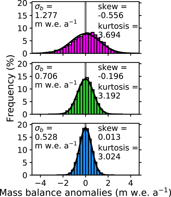
Mass-balance asymmetries stemming from interannual temperature variability should be ubiquitous for glaciers with curvature in their mass-balance profiles, and they should be more acute the larger the curvature and the greater the interannual air-temperature variability. For many glaciers, their mass-balance profiles possess curvature (e.g., World Glacier Monitoring Service (Zemp and others, Reference Zemp2013) or Benn and Evans (Reference Benn and Evans2014), Fig. 3.26), and analysis of multiple glaciological databases indicates that many glaciers have larger mass-balance gradients in their ablation zones than accumulation zones (Rea, Reference Rea2009). The model output from this study can help assess whether these mass-balance asymmetries are easily detectable in the glaciological record. The mass-balance output from the transient simulations for the glaciers with steep and moderate mass-balance gradients appear to be visually different from a normal distribution (Fig. 5). Despite being forced by normally distributed interannual variability, they demonstrate negative skew and are statistically distinguishable from a normal distribution by either a D'Agostino and Pearson (D'Agostino and Pearson, Reference D'Agostino and Pearson1973) or Jarque-Bera test (Jarque and Bera, Reference Jarque and Bera1980) (Fig. 5). The mass-balance output for the glacier with the shallow mass-balance gradient, however, is neither visually nor statistically indistinguishable from a normal distribution (Fig. 5). While this asymmetry should be ubiquitous, its presence in the glaciological record may only be resolvable for glaciers highly susceptible to the asymmetry: glaciers with larger curvature in their mass-balance profile in climates with large interannual air-temperature variability.

Fig. 5. Distribution of mass-balance anomalies for the steep mass-balance gradient glacier (top), moderate mass-balance gradient glacier (middle) and shallow mass-balance gradient glacier (bottom). Normal distributions (black curves) with the same 1 − σ values as the mass-balance times series (σ b) are included. Statistics on the shape of the distribution are also included. The interannual variability is the same as in Fig. 2.
A recent analysis of the World Glacier Monitoring Service (WGMS) database demonstrates that nearly all of the (detrended) mass-balance time series are indistinguishable from normal distributions (Medwedeff and Roe, Reference Medwedeff and Roe2016). In their analysis, 144 out of 158 glaciers (>91%) are statistically indistinguishable from a normal distribution. For tropical glaciers, which have particularly steep mass-balance gradients at lower altitudes, all (n = 6) are indistinguishable (Medwedeff and Roe, Reference Medwedeff and Roe2016). The results of this study, however, suggest that many of the world's glaciers should have skewed mass-balance distributions that should be statistically distinguishable from a normal distribution. The findings from Medwedeff and Roe (Reference Medwedeff and Roe2016) may differ from the analysis of the model output from this study since the length of the time series differs drastically (a few decades vs. 10,000 years). The longest mass-balance record in the Medwedeff and Roe (Reference Medwedeff and Roe2016) study is 67 years, and for tropical glaciers, it is 21 years. Medwedeff and Roe (Reference Medwedeff and Roe2016) note the limited statistical resolving power of the short time series in the WGMS database. Analyses of the model output from this study can help evaluate limitations in the glaciological record.
Using the model output, synthetic mass-balance records are produced that span 10 years, 25 years, 50 years and 100 years. For each time series length, 158 synthetic records are produced. Jarque-Bera tests (Jarque and Bera, Reference Jarque and Bera1980) are used to determine how many of the time series are statistically indistinguishable from a normal distribution. This process is repeated 1,000 times, and the mean and standard deviation (1 − σ) are indicated in Table 2. The ability to statistically resolve the asymmetry increases as the length of the mass-balance record increases. Also, it is more discernible for the glaciers with greater curvature in their mass-balance profiles (Table 2). For 25-year records (longer than any in the tropics), the mass-balance asymmetry can only be statistically resolved ~10% of the time for the glacier with the greatest curvature in its mass-balance profile. The resolving power is even less for the glaciers with less curvature in their mass-balance profiles. These analyses suggest that statistically demonstrating mass-balance asymmetries in glaciological databases will be challenging, even if asymmetries are ubiquitous. The analysis of the WGMS (Medwedeff and Roe, Reference Medwedeff and Roe2016) is not inconsistent with the mass-balance asymmetry presented in this study, and mass-balance asymmetries are likely lurking in the databases. As records become longer, mass-balance asymmetries, such as the one identified in this study and others, should become more statistically discernible.
Table 2. Frequency at which synthetic mass-balance records are statistically indistinguishable from a normal distribution (p ≥ 0.05) by a Jarque-Bera test (same interannual variability as in Fig. 2)
4.3. Mass-balance asymmetries and interpreting changes in glacier length
While changes in average glacier length could be driven by changes in interannual air-temperature, this process may not significantly affect paleoclimatological interpretations of glacier-length changes. Even for large changes in interannual air-temperature variability (25%), length changes are at most a few hundred meters (Fig. 3). An assessment of changes in interannual air-temperature variability during the Medieval Climate Anomaly and Little Ice Age realized in the Paleoclimate Modeling Intercomparison Project Phase 3 (PMIP3) simulations suggests that interannual air-temperature variability changes are at most a few percent (Yang and Jiang, Reference Yang and Jiang2017). Such small changes in interannual air-temperature variability would likely not be noticeable within the spatial resolution of glacier numerical models. Looking further back in time, high-latitude Southern Hemisphere climate variability may have decreased up to 50% between the Last Glacial Maximum (LGM) and the Holocene (Jones and others (Reference Jones2018)). Such a large change in variability might affect LGM paleoclimate reconstructions from glaciers in the mid and high latitudes of the Southern Hemisphere. If temperature variably was substantially elevated during the LGM, then paleoclimate inversions from glacier length changes to changes in climate may somewhat underestimate LGM climate changes, since glaciers may have been smaller than they would be under Holocene-levels of climate variability. For forecasts of glacier evolution over the next century, however, projected changes in interannual air-temperature do not notably affect the forecasts (Farinotti, Reference Farinotti2013). The results of this study also suggest that linear models for glacier-length response to climate forcings can accurately capture the dynamics of transient length fluctuations. The length fluctuations due to interannual variability seem to be well captured as a linear combination of the length fluctuations due to air-temperature and due to precipitation (Table 1). While mass-balance asymmetries likely exist and can affect the mean glacier length, they do not seem to significantly influence the dynamic response of the glacier length to climate changes or impede efforts to reconstruct past climate using changes in average glacier length.
This study may aid paleoclimate modeling studies by helping initialize models for simulations with interannual climate variability. Paleoclimate reconstructions from changes in glacier length should account for both the portion of length changes that could occur due to interannual variability and the portion that requires a change in the climate (Roe, Reference Roe2011; Anderson and others, Reference Anderson, Roe and Anderson2014; Roe and others, Reference Roe, Baker and Herla2017; Herla and others, Reference Herla, Roe and Marzeion2017). Numerical modeling experiments where both interannual climate variability and changes in the climate are explored often simulate these two scenarios independent of each other, in part because the mean length of the glacier changes with the addition of interannual variability (Malone and others, Reference Malone, Pierrehumbert, Lowell, Kelly and Stroup2015; Eaves and others, Reference Eaves, Mackintosh and Anderson2019). In this study, for a constant-width valley, the change in the mean length with the addition of interannual variability can be predicted by time averaging the glacier mass-balance profiles from the transient simulations with variability. This time-averaged mass-balance profiles could then be used to initialize the model before running transient simulations with interannual climate variability and changes in the climate.
5. CONCLUSIONS
This study demonstrates that interannual climate variability can drive transient glacier-length fluctuations, and also partially determines a glacier's average length and mass-balance profile (i.e., its mean state). Interannual variability affects the mean state through a mass-balance asymmetry between warm and cold years that emerges due to curvature in the mass-balance profile. More curvature leads to a larger asymmetry, and this asymmetry grows with increased interannual air-temperature variability. Such asymmetries are also observed for ice sheets (Mikkelsen and others, Reference Mikkelsen, Grinsted and Ditlevsen2018). Mikkelsen and others (Reference Mikkelsen, Grinsted and Ditlevsen2018) used an ice-sheet model that assumes a mass-balance profile with curvature (Oerlemans, Reference Oerlemans2003). Glaciers (or ice sheets) whose mean state is dictated in part by stochastic short-term variability undergo noise-induced drift (Penland, Reference Penland2003). Evidence of mass-balance asymmetries is hard to statistically demonstrate in databases (e.g., the World Glacier Monitoring Service) since records span only a few decades. As mass-balance records become longer, asymmetries should become more discernible.
For reasonable changes in interannual air-temperature variability, the effect on glacier length is minimal -- a few hundred meters at most. These findings, however, may further aid in climatological interpretations of past and present glacier-length changes. Previous paleoclimate reconstructions noting such mass-balance asymmetries have treated the impacts of interannual variability independent from changes to the mean climate (Malone and others, Reference Malone, Pierrehumbert, Lowell, Kelly and Stroup2015; Eaves and others, Reference Eaves, Mackintosh and Anderson2019). Future research should incorporate the role of interannual temperature variability on the mean state of glaciers for both transient and equilibrium simulations. For simple valley geometry used in this study, the change in the mean state can be predicted by time averaging the mass-balance profiles that include interannual variability. These time-averaged vertical mass-balance profiles can provide improved initial conditions for future studies on climatological interpretations of glacier-length changes.
ACKNOWLEDGEMENTS
We thank an anonymous reviewer for feedback on this manuscript and Gerard Roe for feedback on this and an earlier version of this manuscript. This feedback has greatly improved both the presentation and content of this manuscript. AM's funding was provided by the University of Chicago Department of the Geophysical Sciences and the Office of the Provost at Lawrence University. AD's funding was provided by the New Zealand Government under a New Zealand International Research Doctoral Scholarship and through Victoria University of Wellington, in New Zealand. DRM acknowledges grant support from NSF PLR-1443126.
APPENDIX A.
The conditions for a mass-balance asymmetry can be demonstrated using the simplified mass-balance model presented in Roe and O'Neal (Reference Roe and O'Neal2009), which has been utilized subsequently to assess the transient response of glaciers to interannual variability (Huybers and Roe, Reference Huybers and Roe2009; Roe and Baker, Reference Roe and Baker2014; Roe and others, Reference Roe, Baker and Herla2017; Herla and others, Reference Herla, Roe and Marzeion2017). The key assumptions within the Roe and O'Neal (Reference Roe and O'Neal2009) mass-balance model are the same as in this study, except that in this study there is a small accumulation gradient ( 0.1 m w.e. a−1 100 m−1) whereas in the Roe and O'Neal (Reference Roe and O'Neal2009) model there is no accumulation gradient. The mass-balance asymmetry in this study emerges due to the temperature-threshold melt model: Ablation =  $\overline {melt \; rate} \; \times \; melt \; area$. Melt occurs at all evaluations below the ablation season freezing-level-height (
 $A{_{T \gt0^{\circ }{\rm C}}}$) at a melt-rate dictated by how much the air-temperature is above the temperature threshold (0°C). For complete details for the model derivation, please consult Roe and O'Neal (Reference Roe and O'Neal2009).
Assuming the air-temperature follows a linear lapse (Γ) from the summit (x = 0) to the terminus (x = L) and that the glacier has a constant width (w) and is on a constant slope (θ), the ablation model can be expanded as follows:
 $$\eqalign{{\rm Ablation} & = \displaystyle{1 \over 2}\mu (T_0 + \Gamma \;{\rm tan}(\theta )\;L) \cr & \times \left[ {w\;\left(L-\left( {\displaystyle{{-T_0} \over {\Gamma \;{\rm tan}(\theta )}}} \right)\right)} \right]}$$
where T 0 is the summit air-temperature during the ablation season. Equation (A 1) is only valid if the summit air-temperature is below the freezing since otherwise, the ablation area will exceed the area of the entire glacier. If portions of the glacier are below freezing, then there are two mass-balance gradients in the mass-balance profile: (1) a non-zero value in the melt region and (2) a zero value above the freezing-level height. Within both the Roe and O'Neal (Reference Roe and O'Neal2009) model and the methods used in this study, to produce a linear mass-balance profile, the average ablation-season summit air-temperature must be above freezing, in which case the ablation model must be updated so that the melt area does not exceed the total area. The Roe and O'Neal (Reference Roe and O'Neal2009) model can be modified as follows:
 $$\eqalign{&{\rm Ablation} = \cr & \left\{ {\matrix{ {\displaystyle{1 \over 2}\mu (T_0 + \Gamma \;{\rm tan}(\theta )\;L) \times \left[ {w\;\left(L-\left( {\displaystyle{{-T_0} \over {\Gamma \;{\rm tan}(\theta )}}} \right)\right)} \right]} \hfill & {T_0 \lt 0^{\circ} {\rm C}} \hfill \cr {\displaystyle{1 \over 2}\mu (2T_0 + \Gamma \;{\rm tan}(\theta )\;L) \times [w\;L]} \hfill & {T_0 \ge 0^{\circ} {\rm C}} \hfill \cr } } \right.}$$
Perturbing the climate around a mean summit air-temperature: T 0 → T 0 + T′, yields:
 $$\eqalign{ {\rm Ablatio}{\rm n}_{T_{ \lt 0^{\circ} {\rm C}}} &= \displaystyle{1 \over 2}\mu (T_0 + \Gamma \;{\rm tan}(\theta )\;L) \times \left[ {w\;\left(L-\left( {\displaystyle{{-T_0} \over {\Gamma \;{\rm tan}(\theta )}}} \right)\right)} \right] \cr &\quad + \;\mu {T}^{\prime} \times \left[ {w\;\left(L-\left( {\displaystyle{{-T_0} \over {\Gamma \;{\rm tan}(\theta )}}} \right)\right)} \right] \cr &\quad + \;\mu {T}^{\prime} \times \left[ {w\;\left( {\displaystyle{{{T}^{\prime}} \over {\Gamma \;{\rm tan}(\theta )}}} \right)} \right]} $$
 $$\eqalign{{\rm Ablatio}{\rm n}_{T_{ \ge 0^{\circ} {\rm C}}} = & \displaystyle{1 \over 2}\mu (2T_0 + \Gamma \;{\rm tan}(\theta )\;L) \times [w\;L] \cr & + \;\mu {T}^{\prime} \times [w\;L]} $$
In both Eqns (A3) and (A4), the first term ( $ {\cal O}(0)$) describes the ablation for the mean climate, and the second term (
 ${\cal O}(1)$) describes the ablation anomalies due to changes in the melt rate for the melt area for the mean climate. The (
 ${\cal O}(0)$) helps define the mean state, but it is not affected by fluctuations in temperature around the mean. The (
 ${\cal O}(1)$)-term is symmetric and does not affect the mean state. In both this modeling study and the model discussed in the Appendix, an
  ${\cal O}(2)$-term only emerges in the case where the summit air-temperature is below the freezing point (Eqn (A 3)), which is the case where the mass-balance profile has curvature. The
  ${\cal O}(2)$-term is the product of the anomalous melt rate and the anomalous melt area. For a constant valley width glacier, this term grows quadratically with air-temperature perturbations. This
  ${\cal O}(2)$-term is the source of the asymmetry in both this simplified analytical model and the idealized numerical modeling in this study. For the glacier with the constant linear mass-balance profile, the
  ${\cal O}(2)$-term does not appear (Eqn (A 4)), and there would not be a mass-balance asymmetry. The functional form of the asymmetry may differ depending on the valley geometry, but within this study there must be curvature in the mass-balance gradient for there to be a mass-balance asymmetry.


 Open access