Introduction
The city of Amsterdam is situated on the Holocene coastal-deltaic plain of the western Netherlands, at the locality where the small river Amstel joins the IJ. This water body once had a direct connection to the North Sea via the shallow Zuiderzee inlet (Fig. 1), and its geographic position brought Amsterdam a great trading wealth in the 16th and 17th centuries. Land cultivation and peat digging in the city's hinterland provided both food and fuel for rapid expansion. However, adverse subsurface conditions and a surface level very close to sea level also created huge challenges. The shallow subsurface underneath the city consists of over 10 m of unconsolidated Holocene deposits: peat, clay and loosely-packed fine to medium-grained sand. As a result, city development and associated adaptations to the water system led to persistent ground subsidence, in turn affecting buildings and infrastructure. From early on, domestic waste, mud and sand were used to raise the local land surface and to give the city a more firm foundation. Consequently, beneath the city centre the natural surface can nowadays be found at c. –3 to –5 m NAP (= Dutch Ordnance Datum ≈ mean sea level). On top of the natural deposits, up to 5 m of heterogeneous man-made ground occurs, bringing the actual land surface generally just above sea level. Almost all buildings in Amsterdam are founded on piles that usually rest on sand deposits up to several tens of metres deep.

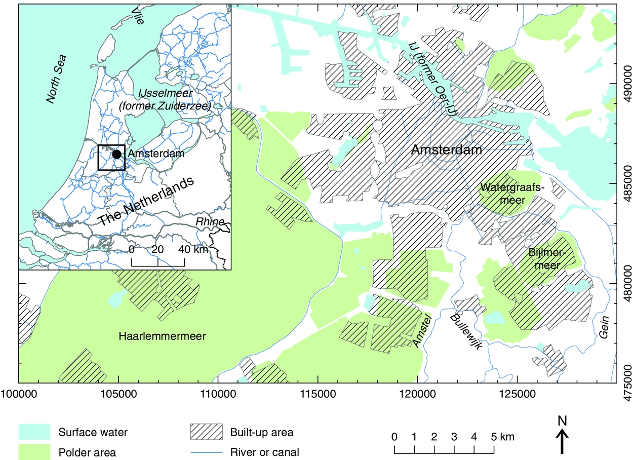
Fig. 1. Location of the study area with localities mentioned in the text.
As in other urban areas, the subsurface of a densely populated city like Amsterdam is nowadays being used with greater intensity, to an increasing depth and for ever more purposes (Anonymous, 2015). The subsoil serves as a storage space for underground infrastructure (cf. Kranendonk et al., Reference Kranendonk, Kluiving and Troelstra2015) and parking, and hosts a dense network of conduits and cables for sewage, drinking water, gas, electricity and other utilities. The subsurface also functions as a groundwater reservoir and is used as energy supply for ground source heat pumps. Apart from that, subsurface space sustains urban nature (e.g. tree rooting) and hosts archaeological heritage. Intensified development of the subterranean space may create more room for functions of city life above ground (Dubbeldam & Souwer, Reference Dubbeldam, Souwer, Borst and Joosten2012). A thorough knowledge of the subsurface of the capital of the Netherlands is therefore vital to sustainable city planning and development (Wentholt & Wolthuis, Reference Wentholt, Wolthuis, Borst and Joosten2012; Van der Meulen et al., Reference Van der Meulen, Doornenbal, Gunnink, Stafleu, Schokker, Vernes, Van Geer, Van Gessel, Van Heteren, Van Leeuwen, Bakker, Bogaard, Busschers, Griffioen, Gruijters, Kiden, Schroot, Simmelink, Van Berkel, Van der Krogt, Westerhoff and Van Daalen2013). The better the structure and properties of the subsurface are understood, the better we can manage the potential and risks of, possibly interfering, below-ground activities.
The Geological Survey of the Netherlands systematically produces 3D subsurface models in which all available basic geological information is integrated to make the most reliable representation of the geological framework beneath our feet (Van der Meulen et al., Reference Van der Meulen, Doornenbal, Gunnink, Stafleu, Schokker, Vernes, Van Geer, Van Gessel, Van Heteren, Van Leeuwen, Bakker, Bogaard, Busschers, Griffioen, Gruijters, Kiden, Schroot, Simmelink, Van Berkel, Van der Krogt, Westerhoff and Van Daalen2013). These so-called geomodels (3D geological models) are also available for the Amsterdam area: the layer-based model Digital Geological Model (DGM; Gunnink et al., Reference Gunnink, Maljers, van Gessel, Menkovic and Hummelman2013) provides general information on the geological units up to a depth of c. 500 m, whereas the voxel model GeoTOP (Stafleu et al., Reference Stafleu, Maljers, Gunnink, Menkovic, Busschers and Busschers2011, Reference Stafleu, Maljers, Busschers, Gunnink, Schokker, Dambrink, Hummelman and Schijf2012) shows, in more detail, the geological units and their lithological properties up to a depth of –50 m NAP. Because all model results are freely available on the internet, anyone interested can use these results to generate customised output for answering specific subsurface-related questions.
The aim of this paper is to explore various aspects of the geology of Amsterdam to a depth of c. 100 m, based on the output of the 3D geological models DGM and GeoTOP. The models are used to create a new geological map of the area, to determine the extent and depth of the foundation levels that have been used for buildings in the city centre and to detect the source of filling sand on which the more recent expansion of the city was largely founded. These examples show that the output of 3D geological models can be directly used to deduce important connections between the subsurface and the natural landscape, historical developments and recent human activities.
Geological setting of Amsterdam
To understand the current geographic setting and subsurface composition of Amsterdam in relation to the historical development of the city, knowledge of the Quaternary geological history is of prime importance. Marine, fluvial, glacial, aeolian and organogenic processes all played their part in this history.
An overview of the lithostratigraphical units that are distinguished in the subsurface of Amsterdam up to a depth of c. –100 m NAP is presented in Table 1. The table lists the main lithological characteristics, depositional environment and chronostratigraphic position of the units, as well as their representation in the geological models DGM and GeoTOP. More extensive information on the properties and characteristics of the lithostratigraphic units can be found on DINOloket (TNO, 2013) and in Westerhoff et al. (Reference Westerhoff, Wong, De Mulder, De Mulder, Geluk, Ritsema, Westerhoff and Wong2003).
Table 1. Lithostratigraphic units in the subsurface of Amsterdam and how these units are represented in the DGM and GeoTOP models (Fig. 3 gives more insight into the distribution, thickness and interrelation of the lithostratigraphic units).

Amsterdam glacial basin
In the late Middle Pleistocene, during the penultimate glacial period (Saalian), glacier tongues at the fringe of a large Scandinavian-based ice sheet formed a series of over 100 m deep glacial basins in the central part of the Netherlands. One of these basins is the Amsterdam glacial basin, a northeast–southwest extending structure with the deepest part in the northeast (Fig. 2). The basin is surrounded by ice-pushed ridges at its western, southern and eastern sides, which were lowered by erosion and denudation processes in subsequent times. The glaciotectonic ridges consist mainly of gravel-bearing, medium to coarse-grained sand of Rhine provenance (Sterksel Formation and Urk Formation) and coarse-grained sand from the north-German fluvial system (Appelscha Formation). The glacial basin later became filled with Late Saalian, Eemian and Weichselian lacustrine, marine, fluvial and aeolian deposits. Holocene siliciclastics and organic deposits finally covered the basin and the surrounding ice-pushed ridges (Fig. 3; e.g. Jelgersma & Breeuwer, Reference Jelgersma, Breeuwer, Zagwijn and van Staalduinen1975; De Gans et al., Reference De Gans, De Groot, Zwaan and van der Meer1987, Reference De Gans, Beets and Centineo2000). Fig. 2 depicts current basin morphology, as indicated by the top depth of the pre-Late Saalian deposits, and shows that the crest of the glaciotectonic ridge is near the surface (situated at c. –2 m NAP) in the southeastern part of Amsterdam. At the western and southern side of the basin the highest parts of the ice-pushed ridges can now be found at –10 to –20 m NAP.

Fig. 2. Morphology of the southern part of the Amsterdam glacial basin and the surrounding ice-pushed ridges, as indicated by the top depth of the pre-Late Saalian deposits. The indicated strike direction of ice-pushed deposits is based on a regional morphological analysis of glaciotectonic landforms.

Fig. 3. West–east cross-section through the Amsterdam glacial basin and surrounding ice-pushed ridges. The indicated strike direction of ice-pushed deposits is based on a regional morphological analysis of glaciotectonic landforms. The location of the cross-section is indicated on Fig. 2. Unit abbreviations refer to Table 1.
Late Saalian deposits (Drente Formation)
Remnants of glacial till occur at the base of the glacial basin sequence. The main part of the Late Saalian infill of the basin consists of (glacio)lacustrine clay and silt, with varves in the deeper parts, deposited in a freshwater lake that probably extended into the present North Sea area (De Gans et al., Reference De Gans, Beets and Centineo2000). At the southern and eastern margin of the basin the fine-grained sediments alternate with medium to coarse-grained sand. This is interpreted as being deposited by small (subaqueous) fans that developed on the oversteepend slopes of the ice-pushed ridges shortly after ice melt.
A cored borehole in the southeastern part of the glacial basin (Core B25G0930: Diemen-Landzicht, Fig. 4; see also De Gans et al., Reference De Gans, Beets and Centineo2000, fig. 5) shows a sand body with large foresets, in total c. 6 m thick. De Gans et al. suggest this unit represents the delta of a river that drained the ice-pushed ridge in the east. An up to 30-m thick sand wedge at the southern rim of the basin has been interpreted as a mass flow deposit (De Gans et al., Reference De Gans, Beets and Centineo2000, fig. 5).

Fig. 4. Core photograph of B25G0930: Diemen-Landzicht, showing silty, shell-bearing clay of the Eem Formation overlying cross-bedded sand of the Drente Formation. The so-called ‘Harting layer’ is lacking in this core. Depth is indicated in metres below surface.

Fig. 5. Relative amount of boreholes at certain depths below the surface for both DGM and GeoTOP in the Amsterdam area.
Eemian deposits (Eem Formation)
On top of the Late Saalian sequence in the deeper parts of the basin (below c. –45 m NAP) a c. 1-m thick sapropel layer occurs that largely consists of diatoms. This diatomite is called the ‘Harting layer’, after Pieter Harting, who first described these sediments in boreholes recovered from the Amersfoort and Amsterdam glacial basins (Harting, Reference Harting1852, Reference Harting1874). The diatomite is overlain by a series of marine clays and silty clays that varies in thickness from a few metres to 30 m (Figs 3 and 4; De Gans et al., Reference De Gans, Beets and Centineo2000). On top of this clayey sequence a series of medium to coarse-grained sands is found that thins towards the southern part of the basin and is thought to have been deposited in a shallow marine, shielded setting.
Weichselian deposits (Kreftenheye Formation and Boxtel Formation)
The Eemian deposits are overlain by a Weichselian series that consists of coarse-grained fluvial sand and fine-grained fluvioperiglacial and aeolian sand intercalated with loam and peat layers. The fluvial sand is only present in the northern and western part of the basin and rests discordantly on the Eemian sand and clay. This sharp transition occurs at a depth of c. –30 m NAP and is sometimes associated with a shell-bearing channel-lag deposit. The coarse-grained sand – with reworked Eemian shells – is assigned to the Kreftenheye Formation. In general, the fluvial deposits gradually grade into fine-grained fluvioperiglacial and aeolian deposits of the Boxtel Formation (Fig. 3; Busschers, Reference Busschers2008).
Holocene succession
In response to climatic amelioration and the melting of the ice caps at the end of the Weichselian, sea level started to rise and the southern North Sea Basin was flooded. The low-lying area in the western Netherlands, including the Amsterdam area, became flooded in the Early Holocene (Beets & Van der Spek, Reference Beets and Van der Spek2000, Fig. 1A; Beets et al., Reference Beets, De Groot and Davies2003). Concurrently with sea level, groundwater level rose, resulting in the development of a widespread peat layer, known as the ‘Basal Peat’, the lowermost part of the Nieuwkoop Formation (Basisveen Bed; Table 1). Currently this peat is consolidated due to the weight of the overlying sediments and has a thickness of 0.2–0.5 m. The peat is conformably overlain by the Velsen Bed, a fine-grained, organic-rich clay with a brackish aquatic fauna (cf. Van Straaten, Reference Van Straaten, Van Straaten and De Jong1957). The Velsen Bed has a thickness of 0.5–2 m. It is in turn overlain by a tidal back-barrier sequence consisting of an over 10-m thick succession of fine- to medium-grained sand and silt, deposited in tidal channels and on tidal flats. These deposits are known as the Wormer Member of the Naaldwijk Formation or as lower tidal deposits (Fig. 3).
Between 5500 and 4500 cal BP the rate of sea-level rise decreased. Along the coastline beach barriers stabilised and formed a so-called ‘semi-closed coast’. The drainage of the hinterland was largely blocked and the former tidal basin developed into a freshwater marsh. The peat that subsequently formed is known as ‘Holland Peat’ (Nieuwkoop Formation, Hollandveen Member).
One west–east oriented tidal channel remained, in connection with the North Sea c. 30 km northwest of Amsterdam. This channel developed into an estuary, the so-called Oer-IJ estuary, draining the hinterland, including the Vecht-Angstel fluvial system (represented by the small river Gein on Fig. 1; cf. Bos et al., Reference Bos, Feiken, Bunnik and Schokker2009). After closure of the inlet by barrier sands the Oer-IJ became a broad extension of the freshwater lakes situated northeast of Amsterdam (see also De Gans, Reference De Gans2015; Vos, Reference Vos2015). From about 1000 AD the lakes gradually widened as a result of shore erosion by wind. Ultimately these growing lakes merged into an inland sea, the Zuiderzee, connected to the North Sea by the Vlie tidal channel in the north (Fig. 1). As a result tidal influence reached the Amsterdam area, not via the west coast but via the distant north coast. With a limited tidal range, storm surges frequently resulted in high water levels, leading to the deposition of thin clay layers on top of the Holland Peat near Amsterdam. Both the Oer-IJ deposits and flood clays are assigned to the Walcheren Member (Naaldwijk Formation), also known as upper tidal deposits.
From c. 3000 years cal BP, Amsterdam became also influenced by the Rhine fluvial system. The river Amstel, originally a local stream draining the peat area, was captured by the Vecht-Angstel fluvial system and thus developed into a northwestern branch of the river Rhine (Bos et al., Reference Bos, Feiken, Bunnik and Schokker2009; De Gans, Reference De Gans2011; Kranendonk et al., Reference Kranendonk, Kluiving and Troelstra2015). Because of its position in the distal part of the delta and the presence of sediment-capturing lakes in the peat area, however, levees along the river remained scarce and narrow, and are only composed of clay and clayey sand. River incision is generally up to a few metres deep into the clastic subsurface. In the centre of Amsterdam, near Dam Square, the river Amstel follows a side branch of the former Oer-IJ tidal channel and reaches a depth of c. –15 m NAP (De Gans & Bunnik, Reference De Gans and Bunnik2011; De Gans, Reference De Gans2015; Kranendonk et al., Reference Kranendonk, Kluiving and Troelstra2015).
Anthropogenic deposits
Building on thick layers of unconsolidated clay and peat combined with improved drainage led to a gradual lowering of the land surface. As a countermeasure, people started to use clay, sand and waste to raise the original surface and keep dry feet. In the 17th century the digging of canals provided material that was deposited directly alongside the canals. In 1870 a law was introduced to further raise the ground on private dwellings (De Gans, Reference De Gans2009). During later town extensions filling sand was applied that was retrieved from the Pleistocene sand deposits outcropping or nearly outcropping around the city, and to a minor extent from the coastal dunes. The thickness of man-made deposits nowadays generally reaches up to 6 m (Fig. 3).
Available subsurface models
To explore the subsurface of Amsterdam, we combined the outcomes of two different geomodels, developed and maintained by TNO, Geological Survey of the Netherlands. Both the Digital Geological Model (DGM) and the GeoTOP model are freely available and accessible through the web portal www.dinoloket.nl. For the purpose of this paper we used DGM v2.2 and GeoTOP v1.2. Basic model specifications are given in this section. More detailed model information can be found in Stafleu et al. (Reference Stafleu, Maljers, Gunnink, Menkovic, Busschers and Busschers2011, Reference Stafleu, Maljers, Busschers, Gunnink, Schokker, Dambrink, Hummelman and Schijf2012), Gunnink et al. (Reference Gunnink, Maljers, van Gessel, Menkovic and Hummelman2013) and on the web portal. Throughout both modelling procedures, internal processes of quality assurance and control on both methodological and geological aspects were performed (cf. Stafleu et al., Reference Stafleu, Maljers, Busschers, Gunnink, Schokker, Dambrink, Hummelman and Schijf2012; Van der Meulen et al., Reference Van der Meulen, Doornenbal, Gunnink, Stafleu, Schokker, Vernes, Van Geer, Van Gessel, Van Heteren, Van Leeuwen, Bakker, Bogaard, Busschers, Griffioen, Gruijters, Kiden, Schroot, Simmelink, Van Berkel, Van der Krogt, Westerhoff and Van Daalen2013). These processes involved various feedback loops and ultimately assured high-quality model output.
DGM
DGM v2.2 is a stacked grid model consisting of raster surfaces that represent the base of 34 lithostratigraphic units in the Dutch onshore subsurface (cf. Gunnink et al., Reference Gunnink, Maljers, van Gessel, Menkovic and Hummelman2013; Van der Meulen et al., Reference Van der Meulen, Doornenbal, Gunnink, Stafleu, Schokker, Vernes, Van Geer, Van Gessel, Van Heteren, Van Leeuwen, Bakker, Bogaard, Busschers, Griffioen, Gruijters, Kiden, Schroot, Simmelink, Van Berkel, Van der Krogt, Westerhoff and Van Daalen2013). The grids are modelled based on the lithostratigraphic interpretation of 26,000 high-quality borehole descriptions spread over the country. Borehole logs and other data such as seismic profiles have been consulted to reconstruct a geological framework used to model the surfaces between data points (Gunnink et al., Reference Gunnink, Maljers, van Gessel, Menkovic and Hummelman2013). Modelling is achieved by geostatistical interpolation methods. The modelled units are mainly at the lithostratigraphic level of formations. Complex or interfingering formations have been combined into a single model unit. This applies, for example, to the Holocene formations and to the Peize Formation and Waalre Formation (see Fig. 3). In the Amsterdam area the maximum model depth is c. –920 m NAP. The reliability of the model is strongly related to the availability (density) of high-quality borehole data. In general at greater depth fewer data points are available and reliability is lower (Figs 5 and 6).
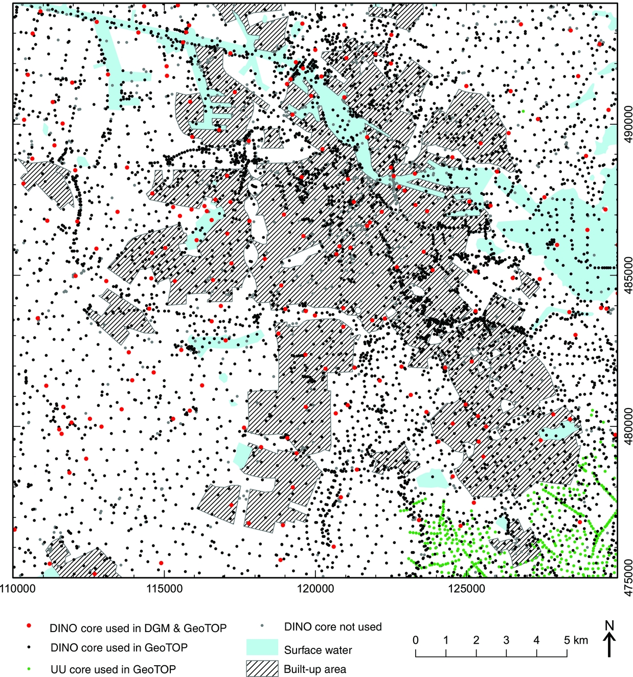
Fig. 6. Geographical overview of the borehole data that were used to construct DGM and GeoTOP in the Amsterdam area.
The model output shows the geometry of the lithostratigraphic units, whereby the top and thickness of each unit have been inferred from the calculated bases. In the upper 100 m of the subsurface of Amsterdam units associated with the Saalian glaciation and the subsequent infilling of the glacial topography are most prominent (Fig. 7).
GeoTOP
GeoTOP v1.2 is a multipurpose, stochastic 3D model that schematises the subsurface into voxels of 100 × 100 × 0.5 m (x, y, z), down to a maximum depth of –50 m NAP (cf. Stafleu et al., Reference Stafleu, Maljers, Gunnink, Menkovic, Busschers and Busschers2011, Reference Stafleu, Maljers, Busschers, Gunnink, Schokker, Dambrink, Hummelman and Schijf2012). In the modelling process each voxel is assigned to the most probable lithostratigraphical unit and lithological class (lithoclass), the latter including sand grain-size classes. As modelling consists of 100 equally probable realisations, uncertainties regarding these parameters are also provided (Stafleu et al., Reference Stafleu, Maljers, Gunnink, Menkovic, Busschers and Busschers2011, Reference Stafleu, Maljers, Busschers, Gunnink, Schokker, Dambrink, Hummelman and Schijf2012; Van der Meulen et al., Reference Van der Meulen, Doornenbal, Gunnink, Stafleu, Schokker, Vernes, Van Geer, Van Gessel, Van Heteren, Van Leeuwen, Bakker, Bogaard, Busschers, Griffioen, Gruijters, Kiden, Schroot, Simmelink, Van Berkel, Van der Krogt, Westerhoff and Van Daalen2013). Starting from the province of Zeeland in 2007, GeoTOP modelling has since progressively covered the western, central and northern part of the Netherlands. The subsurface of Amsterdam became the focus in 2011 as part of the modelling of the province of Noord-Holland.
The main data source of the GeoTOP model is the fast-growing number of digital borehole descriptions in the database Data en Informatie van de Nederlandse Ondergrond (DINO). From the total number of digital borehole descriptions that was available in DINO at the time, c. 85% was of sufficient quality to be used to build the GeoTOP model of the Amsterdam area. This dataset was complemented by borehole data from Utrecht University, gathered within the framework of long-lasting research on the Holocene development of the Rhine-Meuse delta (Berendsen & Stouthamer, Reference Berendsen and Stouthamer2001; Bos et al., Reference Bos, Feiken, Bunnik and Schokker2009; Cohen et al., Reference Cohen, Stouthamer, Pierik and Geurts2012). In total 6225 borehole descriptions have been used to build the model. This amounts to 15.34 borehole descriptions per square kilometre. As is the case with DGM, at greater depths below the surface the number of available borehole descriptions per square kilometre decreases rapidly (Fig. 5).
Before modelling of a new area starts, a conceptual model of the subsurface is constructed. The conceptual model shows the lithostratigraphical units that can be recognised in the modelling space and depicts their mutual stratigraphical relationships. A list of modelled units that are of interest in the Amsterdam area can be found in Table 1. Subsequently, information is gathered on the spatial distribution of the different units. The spatial distribution of most of the deeper Pleistocene units is directly derived from the DGM model. For the shallow Holocene units, spatial information is derived from various sources, including the available geological, soil and geomorphological maps on a scale of 1:50,000. The spatial distribution of anthropogenic deposits is derived from a national land-use map (Landelijk Grondgebruik Nederland; www.lgn.nl).
The modelling itself involves three basic steps (Stafleu et al., Reference Stafleu, Maljers, Gunnink, Menkovic, Busschers and Busschers2011, Reference Stafleu, Maljers, Busschers, Gunnink, Schokker, Dambrink, Hummelman and Schijf2012):
-
1. Borehole information is coded lithostratigraphically and in terms of lithoclasses.
-
2. The basal surface of each lithostratigraphical unit is modelled in two dimensions using sequential Gaussian simulation techniques.
-
3. The lithoclasses within each lithostratigraphical unit are modelled in three dimensions using sequential indicator simulation techniques.
Although both modelling steps 2 and 3 result in 100 model realisations, we only used the most probable model outcome in this study (Fig. 8).
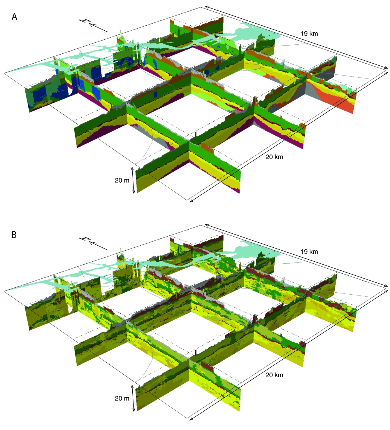
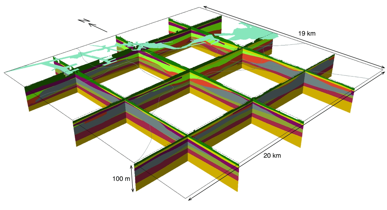
Fig. 8. Fence diagram through part of GeoTOP up to a depth of –20 m NAP. The lateral extent of the model blocks is equal to Fig. 10. A. Lithostratigraphic units. See Table 1 for an explanation of the units and associated colours. B. Lithoclasses. Brown, peat; dark green, clay; light green, sandy clay/clayey sand/loam; yellow to orange, sand in three different grain-size classes; grey, anthropogenic deposits'.
Differences between DGM and GeoTOP
DGM is a nationwide model that is very useful to get a general overview of the subsurface and enables the deeper layers to be surveyed and analysed. It also forms the basis of REGIS II, a nationwide hydrogeological model of the Dutch subsurface (Vernes & Van Doorn, Reference Vernes and Van Doorn2005). GeoTOP provides more detail in the upper 30–50 m of the subsurface. It is able to depict the Holocene lithostratigraphical formations, members and beds as separate entities, rather than one amalgamated unit. This is possible because the model makes use of almost all available digital borehole descriptions in DINO (cf. Fig. 6). Furthermore, GeoTOP not only provides information on the architecture of the geological units in the subsurface (step 2 in the modelling procedure of GeoTOP), but also on the distribution of lithological properties within these units (step 3). Within the ice-pushed ridges, the dip of the glaciotectonised strata has been used to properly model the lithoclass distribution (Stafleu et al., Reference Stafleu, Maljers, Busschers, Gunnink, Schokker, Dambrink, Hummelman and Schijf2012).
Exploring the subsurface using models
Many questions regarding the shallow geology of Amsterdam can be answered using customised 2D raster maps, created by simple calculations on the 3D model data. This section shows three examples of this approach. Whereas it is rather straightforward to create maps from a layer-based model such as DGM (see Example 2), querying voxel stacks is a valuable tool when deriving information from a voxel model such as GeoTOP (see Examples 1 and 3; Stafleu et al., Reference Stafleu, Maljers, Busschers, Gunnink, Schokker, Dambrink, Hummelman and Schijf2012).
A voxel stack represents the vertical sequence of one or more voxel properties at a particular location (x, y) (Fig. 9). From analysing the stack, the value of a voxel property at a specific depth can be deduced. Likewise, the vertical sequence of a voxel property value can be inferred (e.g. the sequence of lithostratigraphic units, see Example 1). In addition, the depth can be calculated at which a specific combination of voxel property values occurs (e.g. the uppermost occurrence of a particular lithoclass within a specific lithostratigraphic unit, see Example 3). All examples presented here are a direct outcome of querying 3D model data.

Fig. 9. A hypothesised vertical voxel stack with two properties: lithostratigraphic unit and lithoclass. The uppermost occurrence of two consecutive sand voxels within lithostratigraphic unit NAWO is found at 3.5 m below surface.
Example 1: Geological map of Amsterdam
The former State Geological Survey (Rijks Geologische Dienst) and its predecessor published the Geological Map of the Netherlands in a series of 1:50,000 paper map sheets during the period 1964–2000. Each map sheet was accompanied by one or more subsidiary maps, vertical cross-sections and a comprehensive memoir, describing the geology of the area in detail. In the coastal area, the main map was composed using a so-called profile-type legend (De Jong & Hageman, Reference De Jong and Hageman1960; Hageman, Reference Hageman1963). This implies that each map unit refers to a well-defined sequence of geological units, thus enabling the depiction of the 3D arrangement of deposits in two dimensions.
The Geological Map of the Netherlands on a 1:50,000 scale was never finished. After 46 years of work, the last map sheet was published in 2000. By then around 30% of the Netherlands had been covered. The two map sheets that cover Amsterdam (24/25W and 25O) have not been published, although field activities have been completed and a concept map was constructed. As such, the last official geological map that covers the Amsterdam area dates from 1926 to 1928 (Map sheets 25 I to IV; Tesch, Reference Tesch1926, Reference Tesch1927a,Reference Teschb, Reference Tesch1928). Apart from conceptually being outdated, these map sheets and their accompanying vertical cross-sections show the situation of the 1920s and mainly provide information on the upper 2 m of the subsurface.
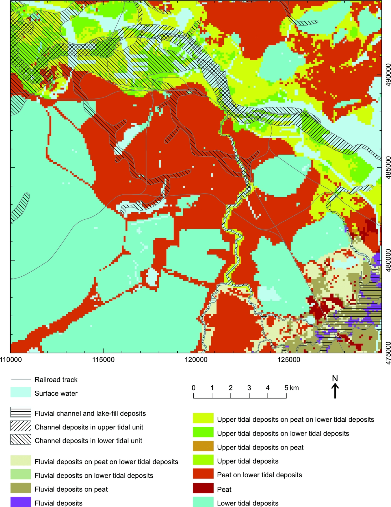
Using GeoTOP, an up-to-date geological map of Amsterdam and surroundings has been constructed (Fig. 10). This has been achieved by querying the individual voxel stacks and has led to a map with a profile-type legend similar to that used on the 1:50,000-scale maps. Probing down from each surface grid cell, the sequence of Holocene geological units was obtained. In first instance, this resulted in 414 different sequences, featuring 11 geological units. The number of sequences was subsequently reduced by:

Fig. 10. Geological map of the Amsterdam area based on GeoTOP voxel stack calculations.
-
• omitting the anthropogenic deposits at the top of the stack
-
• combining the different generations of channel deposits with their respective mother units (e.g. the channel deposits of the upper tidal unit were combined with the other deposits of the upper tidal unit)
-
• combining the Velsen Bed with the remainder of the Wormer Member into the lower tidal unit
-
• omitting the Basisveen Bed at the bottom of the stack.
Because the channel deposits in GeoTOP (see Stafleu et al., Reference Stafleu, Busschers, Maljers, Gunnink, Berg, Russell and Thorleifson2009, Reference Stafleu, Maljers, Gunnink, Menkovic, Busschers and Busschers2011, Reference Stafleu, Maljers, Busschers, Gunnink, Schokker, Dambrink, Hummelman and Schijf2012) are modelled separately, the stratigraphy of the channels is not entirely consistent with the stratigraphy of the remainder of the model. In rare cases, for example, the top of a young tidal channel may fall below the bottom of the upper tidal unit. Combining the channel deposits with their mother units therefore occasionally resulted in incorrect, overcomplicated sequences. These were simplified, obeying the stratigraphic model of the area (cf. Table 1). Ultimately, this has led to a map with 11 profile-type legend units, composed of stacks of four geological units: fluvial deposits, upper tidal deposits, Hollandveen peat and lower tidal deposits. The modelled fluvial channel and lake-fill deposits and upper and lower tidal-channel deposits have subsequently been superimposed on the map. The extent of these units was derived from a combination of non-published and external data sources, including Steur & Heijink (Reference Steur and Heijink1965) and Bos et al. (Reference Bos, Feiken, Bunnik and Schokker2009).
The geological map shows the dominance of peat and tidal deposits within the Holocene sequence below Amsterdam. In the city centre, and covered by 2–5 m of anthropogenic deposits (Fig. 3), peat (Nieuwkoop Formation, Hollandveen Member) overlies lower tidal deposits (Naaldwijk Formation, Wormer Member). Around the IJ in the north, this sequence is overlain by upper tidal deposits (Naaldwijk Formation, Walcheren Member), a result of deposition from both the northwest (Oer-IJ estuary) and northeast (Zuiderzee). Southwest and south of Amsterdam, the former lakes of Haarlemmermeer, Bijlmermeer and Watergraafsmeer are apparent, where the peat has been eroded and the lower tidal deposits are the uppermost natural deposits in the subsurface. On the southeastern part of the map, fluvial deposits of the Vecht-Angstel and Amstel systems occur in most of the units. In accordance with the 1:50,000 soil map (Steur & Heijink, Reference Steur and Heijink1965), but contrary to recent findings of De Gans & Bunnik (Reference De Gans and Bunnik2011) and De Gans (Reference De Gans2015), the clayey deposits surrounding the river Amstel north of the confluence with the small river Bullewijk have been mapped as tidal deposits. This young system follows an older tidal channel along the middle part of its course (Fig. 10). It may be argued that this is the result of the higher erodibility of the clayey sand deposits of the tidal channel in comparison with the surrounding, more clayey deposits (cf. De Gans & Bunnik, Reference De Gans and Bunnik2011).
Although the geological map published here largely follows the profile-type legend of the original 1:50,000 geological maps, the direct derivation of the new map from GeoTOP allows for a quick and easy adaptation to any tailored legend system desirable. The output could, for instance, be modified to show the presence or absence of one specific unit, to show the unit sequence above or below a certain unit, and so forth. It is also possible to construct a map with a profile-type legend based on the sequence of lithoclasses rather than geological units. In short, all these possibilities enable the distillation and presentation of a wide variety of shallow-subsurface information, which is in contrast to the rather limited set of subsidiary maps that used to be published in association with the 1:50,000 map sheets.
Example 2: Aggregate resources
The Amsterdam area is part of the low-lying and flat landscape that typifies the western part of the central Netherlands. This morphology differs from the central and eastern part of the country, where ice-pushed ridge complexes, or push moraines, stand out in an otherwise rather flat landscape. The highest ridges are generally present in the east. Towards the west the ridges are lower, which is mainly related to large-scale erosion and long-term tectonic subsidence. As a result, the westernmost ridges are presently buried under younger deposits. The Muiderberg ridge is often considered the westernmost outcrop of ice-pushed sediments. However, prior to the expansion of Amsterdam towards the southeast, Bennema (Reference Bennema1951) mapped Pleistocene sand at or very close to the surface in the low-lying polders Bijlmermeer and Gein en Gaasp. This sand represented, in fact, the westernmost Pleistocene outcrop in the central Netherlands. Also further to the west the highest parts of the buried ice-pushed sediments occur relatively close to the surface. These deposits have proven to be a valuable source for raw mineral extraction during the 20th-century expansion of Amsterdam (e.g. Vonk, Reference Vonk2000). The wet sand and gravel extraction pits of Gooimeer, Oudekerkerplas, Nieuwe Meer and Sloterplas, with water bottom depths down to –35 m NAP, were all created in this period.
When comparing the pattern of sand and gravel extraction pits with the results of DGM, it becomes apparent that the pits line up in a semi-circular pattern around the city, largely coinciding with the arched presence of ice-pushed ridge deposits at shallow depths (Fig. 11). In a similar way, the location of the arch of ice-pushed ridges gives a first insight into those aggregate resources potentially available for dredging in the near future, providing present-day land use and other regulations do not inhibit extraction. A more detailed resource assessment can subsequently be performed on the web portal www.delfstoffenonline.nl (see also Van der Meulen et al., Reference Van der Meulen, Van Gessel and Veldkamp2005; Maljers et al., Reference Maljers, Stafleu, van der Meulen and Dambrink2015).

Fig. 11. Location and depth of generally coarse-grained ice-pushed ridge deposits in relation to historical aggregate resource extraction locations.
Example 3: Foundation levels
Due to the weak subsurface, the city of Amsterdam has been built on millions of foundation piles. It is said that the Royal Palace (built as Amsterdam City Hall in 1655) was originally founded on a total of 13,659 piles. The piles below the palace that have been examined are made of wood from Pinus sylvestris (Scots pine) and Picea abies (Norway spruce), imported from both the Baltic area and central Germany (Van Tussenbroek, Reference Van Tussenbroek2012). Piles below modern buildings often consist of reinforced concrete or steel. Without these piles, buildings would sink down slowly under their own weight or possibly eventually collapse due to differential subsidence. Following from past building experience, in the city centre four distinct foundation levels are discerned (De Gans, Reference De Gans2011; cf. Fig. 3):
-
• Boerenzand (‘Farmer's sand’): Clayey sand level in the Middle Holocene lower tidal deposits. Originally used as a foundation level for the old, wooden buildings.
-
• First foundation level: Late Pleistocene coversand (Boxtel Formation, Wierden Member). Used as a foundation level for, for example, the Royal Palace (1655).
-
• Second foundation level: Late Pleistocene fluvial sand (Kreftenheye Formation) and marine sand (Eem Formation). Used as a foundation level for, for example, De Nederlandsche Bank (1968).
-
• Third foundation level: Middle Pleistocene fluvial sand (Urk Formation, Sterksel Formation or ice-pushed deposits). Used as a foundation level for, for example, the North–South line metro station below Amsterdam Central Station (currently under construction).
Although the depth of these foundation levels is more or less known, the lateral continuity of the levels is not very well established. It is known for example that the first foundation level can be absent due to erosion by Holocene tidal processes. Also, the foreseen foundation levels may appear too thin to act as a firm foundation or locally consist of non-sandy material. Taking this into consideration and based on the results of GeoTOP we applied the following characteristics to define a foundation level:
-
• A foundation level consists of at least two stacked sand voxels (i.e. a 1-m thick sand layer).
-
• The geological unit of the voxels is used to discern between the different foundation levels.
-
• In case of the Boerenzand, the sand layer should not be underlain by 2 m or more of poorly consolidated Holocene deposits. If this is the case, the sand is considered not to be suitable for foundation.
The resulting maps (Fig. 12) show the extent and top depth of each of the four levels. The extent of the Boerenzand (–6 to –8 m NAP; Fig. 12A) is rather patchy and appears to be related to the tidal-channel pattern in the lower tidal deposits. Close to the channels, the Boerenzand level is often absent, suggesting that the clayey sand reflects a sandy tidal flat facies rather than a channel facies (cf. Beets et al., Reference Beets, De Groot and Davies2003). Also in the city centre the foundation level is largely absent, or at least does not confirm to the specifications above.

Fig. 12. Maps showing extent and depth of four different foundation levels below Amsterdam. A. Boerenzand. B. First foundation level. C. Second foundation level. D. Third foundation level. See text for definition of the different levels. 1, Royal Palace; 2, De Nederlandsche Bank; 3, Amsterdam Central Station.
In contrast to the Boerenzand, the first foundation level is present throughout the area (Fig. 12B). Only the very deep tidal channels around the IJ estuary have eroded the coversand in the uppermost part of the Pleistocene deposits. The level is generally found at –11 to –13 m NAP, but close to the Amstel, green colours indicate a much deeper foundation level at the base of the Boxtel Formation at –18 to –20 m NAP. Although a thin coversand layer is present here, it is directly underlain by clay and peat from the Weichselian Pleniglacial, locally known as the Intermediate Level (cf. De Gans & Wassing, Reference De Gans and Wassing2000). The coversand above is therefore not considered to be a firm foundation level.
The second foundation level occurs at a depth of –17 to –26 m NAP (Fig. 12C). To the south and east of the city centre, however, this level is largely absent. During the Eemian transgression, this part of the Amsterdam glacial basin became for the large part filled with marine clay, not suitable as a firm foundation.
The third and deepest foundation level reflects the glacial basin morphology (Fig. 12D). Below the city centre, this foundation level occurs deeper than –50 m NAP. Towards the basin edges, the level quickly rises up to depths shallower than –20 m NAP. Mapping of this foundation level suggests the presence of a glacial-basin outflow to the southwest, with a sill height of approximately –30 m NAP. Although the presence and supposed glaciofluvial origin of this sill need to be confirmed by detailed examination of site data, this is an example of the type of geological insights that can be derived from geomodelling.
Discussion and implications
Application of model results
Results of DGM and GeoTOP modelling are freely available to the public via DINOloket in a variety of ways: through a web viewer, as data files for SubsurfaceViewer (www.subsurfaceviewer.com) and as dedicated ASCII grids and shape files. For this paper, GeoTOP voxel-stack calculations were performed directly on the ASCII model output. These calculations enabled the construction of a geological map of Amsterdam with a profile-type legend and the reconstruction of foundation level geometries. The lateral extent and top depth of DGM model units combined with the historical locations of aggregate resource extraction enabled inferences to be made about the source of material that was taken out as aggregate resource during the 20th century city extensions.
With these examples it is shown that custom-made products can be derived from the modelling results. Model resolution particularly enables application of the results in the early stage of research or the planning stage of an applied project, geotechnical, hydrological or otherwise. As such, these outcomes do not replace detailed ground investigations. The advantage of using the models is particularly found in the quick and easy way by which the model results can provide general insight into a particular problem.
GeoTOP modelling results in multiple, equiprobable realisations of the subsurface lithology. This enables the calculation of modelling uncertainties. In the present case studies only the most probable model outcomes were used. By taking into account the associated uncertainties, the calculations and final results could be refined and statistically quantified.
GeoTOP, which includes the information of the vast majority of currently digitally available borehole data, together with expert knowledge and legacy data of many different parties, currently provides the best available representation of the subsurface and its lithological properties at a regional level. To improve the possibilities of applying geomodels when dealing with detailed questions regarding the urban subsurface, model resolution could be further enhanced. This could be achieved by integrating other data types, such as cone-penetration test (CPT) data in the modelling procedure. In general, CPT data are much more widely available than core descriptions. Also, the use of additional data sources, apart from the database DINO, e.g. municipal databases, could improve data density and thus allow for higher-resolution models. Other possible advances are enhanced mapping and characterisation of man-made ground and the visual combination and, eventually, model integration of geological subsurface data with other types of subsurface data and above-ground information.
Geological implications
In addition to the possibilities of a tailor-made analysis and presentation of subsurface data using geomodels, geological implications can be derived from the model results. These include the following:
-
• The river Amstel follows an older tidal channel along part of its course. This might be the result of a higher erodibility of the clayey sand deposits of the channel fill in comparison with the surrounding, more clayey deposits.
-
• The coarse-grained ice-pushed ridge deposits encircling Amsterdam at shallow depth still give ample opportunities for the future extraction of aggregate resources, providing present-day land use and other non-geological boundary conditions do not inhibit this.
-
• The Amsterdam glacial basin probably has an outflow to the southwest, with a sill height of approximately –30 m NAP.
-
• The extent of the Boerenzand is shown to be rather patchy and appears to be related to the tidal-channel pattern in the lower tidal deposits. Close to the channels, the Boerenzand clayey sand level is often absent. This suggests that the clayey sand reflects a sandy tidal flat facies rather than channel facies.
All the above findings show that subsurface conditions have had a profound effect on both landscape development and the expansion of the city of Amsterdam from the Middle Ages onwards. In order to understand city development in a coastal-deltaic setting, it is therefore crucial to obtain information about the geological history of the locality and the resulting subsurface architecture. Geomodels like DGM and GeoTOP provide an easily accessible way of obtaining this information.
Acknowledgments
We are grateful to Wim de Gans and two anonymous reviewers for their comments on an earlier draft of this paper. Our colleagues at the Geomodelling Team are thanked for stimulating discussions on both modelling and the geology of the Netherlands. This paper was established within the framework of COST Action Sub-Urban (TU1206), a European network to improve understanding and the use of the ground beneath our cities (www.sub-urban.eu).