THE SOLAR MINIMUM CORONA FROM DIFFERENTIAL EMISSION MEASURE TOMOGRAPHY

Over the last four decades, our understanding of the physics of the highly inhomogeneous and structured solar corona has experienced sustained advance, thanks to the many observational, theoretical, and modeling efforts, which strengthened over the past two decades, and to the many simultaneously operational solar-dedicated space missions, and their diverse observational capabilities. In spite of the many advances, the increasingly extensive data sets imply that further development of models is required to improve their ability to match different observations and, hence, to achieve a better understanding of the underlying physical mechanisms. A path for further advance in models then lies in the assimilation of as much comprehensive empirically derived information as possible. In particular, the latest generation of three-dimensional (3D) magnetohydrodynamical (MHD) models of the corona would greatly benefit from 3D empirically derived maps of the fundamental plasma parameters, the electron density, and temperature. This is especially so at the lower corona, where some of the energy release mechanisms take place, as coronal heating, wind acceleration, and coronal mass ejection (CME) generation. In this context, we have recently developed a novel technique, named Differential Emission Measure Tomography (DEMT), that produces maps of the 3D EUV emissivity, and of a 3D version of the standard DEM analysis but without projection effects. This local DEM (or LDEM) analysis allows in turn the derivation of 3D maps of the electron density and temperature (Frazin et al. 2009). We have already presented results derived from the application of this technique, initially proposed by Frazin et al. (2005), to Solar Terrestrial Relations Observatory (STEREO)/Extreme Ultraviolet Imager (EUVI) data (Vásquez et al. 2009). In that work we published the first empirically derived 3D density and temperature structure of coronal filament cavities, known to be the source region of about 2/3 of all observed coronal mass ejections (CMEs; Gibson et al. 2006). In this work, we focus on the large-scale characteristics of EUV tomographic reconstructions during the last solar minimum.

One of the primary goals of NASA's dual-spacecraft STEREO mission is precisely to determine the 3D structure of the corona (Kaiser et al. 2008). The EUVI on the STEREO mission returns high-resolution (16) narrowband images centered over Fe emission lines at 171, 195, 284 Å, and the He ii 304 Å line (Howard et al. 2008). DEMT takes advantage of the solar rotation to provide the multiple views required for tomography, as well as of the dual view angles provided by the STEREO spacecraft. A major advantage of the technique is the lack of need for ad-hoc geometrical modeling of any structure of interest. Its main (current) limitation is the assumption of a static corona during the data gathering process, implying that the reconstructions are reliable only in coronal regions populated by structures that are stable throughout their disk transit in the images. The use of the two view angles of STEREO allows for a reduced data gathering time. In this work we apply DEMT to STEREO/EUVI data corresponding to the last extended solar minimum, specifically to Carrington Rotation (CR) 2077. The results of the DEMT technique span the effective height range 1.035–1.225 R_s. By tracing out the PFSS model field lines through the tomographic computational volume, we are able to identify in particular the magnetically open and closed regions. Comparison of the DEMT and PFSS results allows the construction of a large-scale low corona model for the electron density and temperature. We discuss the implication of our model for the thermodynamical structure of the equatorial streamer belt, as well as for the surrounding magnetically open regions, generally considered to be source of part of the slow component of the solar wind (Suess et al. 2009).

A comprehensive discussion of the procedures here summarized can be found in Frazin et al. (2009). In the optically thin limit, the (instrument-specific units) intensity I_k,j in the jth image pixel of the kth EUV spectral band can be shown to be related to the filter band emissivity (FBE) ζ_k through

$$\begin{equation} I_{k,j} = \Phi _{k,0} \int _{\mathrm{LOS}} {d} l \ \zeta _k [{\bf r}_j(l)] \, + n_{k,j} \,, \end{equation} \tag{ 1 }$$

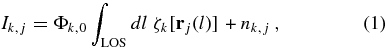
where n_k,j is the noise in the measurement, r_j(l) is a vector that traces out the line of sight (LOS) corresponding to the jth image pixel as a function of the scalar parameter l, and Φ_k,0 is a conversion factor that transforms from physical intensity units into the instrument-specific signal units. The FBE ζ_k is related to the plasma emissivity η and the filter transmittance ϕ_k(λ) through the wavelength (λ) integral:

$$\begin{equation} \zeta _k ({\bf r}) = \int {d} \lambda \ \phi _k(\lambda)\ \eta (\lambda ; {\bf r}) \,. \end{equation} \tag{ 2 }$$

After discretization of the coronal volume, Equation (1) provides an independent tomographic problem for each band k, that can be solved for the FBE through global optimization techniques. The solution of the problem involves the application of regularization (or smoothing) methods to stabilize the inversion. In the case of this work, the regularization is implemented through the inclusion of the norm of the angular second derivatives matrix into the cost function of the global optimization problem. The amplitude of this term is controlled by a single regularization parameter p, and its value is determined via the statistical procedure of cross validation, discussed below in Section 3 (see also Frazin et al. 2009; Frazin & Janzen 2002). As Equation (1) does not account for the Sun's temporal variations, fast dynamics in the region of one grid cell (or voxel) can cause artifacts in neighboring ones. Such artifacts include smearing and negative values of the reconstructed emissivity, or zero when the solution is constrained to positive values. These are called zero-density artifacts (ZDAs), and are similar in nature to those described by Frazin & Janzen (2002) in the context of white light tomography. The constructions are then reliable for structures that remain stable during the time that they are seen by the telescopes. The issue of temporal variation in SRT is addressed in Frazin et al. (2005).

Using only one instrument, a tomographic problem requires gathering data during a full synodic rotation. In the case of reconstructions performed with STEREO/EUVI, the use of data taken by both instruments at the same time allows for a reduced data gathering time due to the angular separation of their view angles. The simultaneous use of two (or more) instruments requires enough similarity between the different telescopes, which is a fulfilled requirement in this case (see Frazin et al. 2009). Another important benefit of the multi-spacecraft tomography relies on the increased opportunities for cross validation due to the existence of a range of redundant observational angles (i.e., observational angles that have been covered by both instruments).

A main assumption of the tomographic technique is the optically thin regime of the corona for the observed radiation. This is fulfilled by the three EUVI coronal bands in most regions. The image pixels that are likely to be severely affected by an optically thick regime are those near the disk limb. This is caused by the tangential inclination with which the LOSs of those pixels pass through the corona. We developed a statistical data rejection procedure, fully detailed in Frazin et al. (2009), to establish what part of the images is not to be used for tomography. We determine that pixels with projected radii between 0.98 and 1.025 R_s are to be rejected. As a result, our EUV tomographic reconstructions are not physically meaningful between 1.0 and 1.025 R_s. Due to the finite extension of both the EUVI field of view and the tomographic computational grid, both set equal to 1.25 R_s in this work, there is an artificial material build-up for the results in the outer layers of the computational grid, specifically above 1.235 R_s. The EUVI instruments include also a band centered around the 304 Å He line, which is optically thick, and hence these tomographic reconstructions are not useful for any quantitative purposes. Still, in the 304 case we perform hollow reconstructions (i.e., blocking out all image pixels bellow 1.01 R_s) in order to construct qualitative maps of chromospheric material above the limb, or prominences, which are very bright in this emission line. This has proven to be extremely useful to interpret data from the Fe band reconstructions, allowing association of the reconstructed coronal features with underlying prominences, as shown in Vásquez et al. (2009).

As with all optical instruments, the image measured by EUVI can be modeled as a convolution of the true solar image (as would be seen by an ideal telescope) with the instrument point-spread function (PSF). The EUVI PSF is different in each band, but in all cases, results from a combination of non-specular scattering off the mirror, which gives rise to broad wings and a complex diffraction pattern due to the aperture and obstructions. These broad wings of the PSF have important consequences for the Sun's fainter structures such as coronal holes (CHs) and emission at larger heights above the limb. Our preliminary analysis shows that, depending on the band, up to about 50% of the emission seen in CHs is due to the PSF. Since our deconvolution procedures are not yet ready for deployment, we do not analyze CHs here.

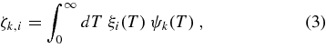
As shown in Frazin et al. (2009), the K tomographic FBEs in the ith voxel, ζ_k,i, are linearly related to the LDEM ξ_i(T) through the respective band temperature response function ψ_k(T) of the instrument,

$$\begin{equation} \zeta _{k,i} = \int _0^\infty {d} T \ \xi _i(T) \ \psi _k(T) \;, \end{equation} \tag{ 3 }$$

where T is the electron temperature and the function ψ_k(T), proportional to the kth band spectral emissivity, is computed from an optically thin plasma emission model such as CHIANTI. The temperature responses of the two EUVI instruments, displayed in Figure 2 of Frazin et al. (2009), have sensitivity peaks at about 0.86, 1.43, and 2.08 MK, for the 171, 195, and 284 Å bands, respectively. The LDEM is proportional to the squared electron density N²_e, and gives a measure of the amount of plasma as function of temperature within the voxel. The K = 3 coronal bands of EUVI do not provide enough information to invert Equation (3) for a general LDEM functional form. We therefore assume a Gaussian LDEM in each voxel: $\xi _i(T) = \mathcal {N}\left(T;[T_0, \sigma _T, a]_i\right)$, where T₀, σ_T, and a are its centroid, 1/e width, and amplitude, respectively. At each voxel, these parameters are determined by minimizing the discrepancy between the three tomographically reconstructed values ζ_k,i and $\int {d} T \, \mathcal {N}\left(T;[T_0, \sigma _T, a]_i\right) \psi _k(T)$ (Vásquez et al. 2009). Based on the distribution ξ_i(T) we determine in each computational grid cell i, we can compute its zeroth through second moments,

$$\begin{eqnarray} \left< N_e^2\right>_i &=& \int _{T_{\rm min}}^{T_{\rm max}}{d} T \, \xi _i(T) \,, \end{eqnarray} \tag{ 4 }$$

$$\begin{eqnarray} T_{m,i} \ \equiv \ \langle T_e\rangle _i &=& \frac{1}{\big< N_e^2\big>_i } \int _{T_{\rm min}}^{T_{\rm max}}{d} T \, \xi _i(T)\, T \,, \end{eqnarray} \tag{ 5 }$$

$$\begin{eqnarray} W_{T,i}^2\ \equiv \ \langle (\Delta T_e)^2 \rangle _i &=& \frac{1}{\big< N_e^2\big>_i } \int _{T_{\rm min}}^{T_{\rm max}}{d} T \, \xi _i(T) \, (T-T_{m,i})^2 \,,\quad \ \ \end{eqnarray} \tag{ 6 }$$

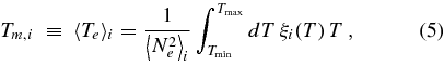
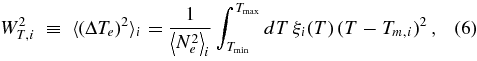
where the integrals are taken over the EUVI bands sensitivity range T:[0.5, 3.5] MK. For the ith voxel, these quantities are the mean squared electron density, mean electron temperature, and squared electron temperature spread, respectively. As the EUVI coronal bands are dominated by iron lines, their temperature responses are proportional to that element abundance, and hence the LDEM and rms N_e value derived at each voxel are inversely proportional to it. In this work we assume the iron abundance to be uniform and equal to [Fe]/[H] = 1.26 × 10⁻⁴ (Feldman et al. 1992), a low first ionization potential (FIP) element abundance enhanced by a factor of about 4 with respect to typical photospheric values (Grevesse & Sauval 1998). We also assume for the Fe ions the results given by the ionization equilibrium calculations of Arnaud & Raymond (1992). One must hence bear in mind that all results for density gradients given below could be partly ascribed to abundance variations. The average temperature T_m and the temperature spread W_T are not affected by the Fe abundance. On the other hand, the degree of contamination of dim regions due to the PSF contamination is expected to differ for the different bands, and this changes the LDEM and its moments.

We use STEREO/EUVI A and B data simultaneously taken during Carrington rotation (CR) 2077 (UT 2008 November 20 06:56 through UT December 17 14:34). During this period, the two spacecraft were separated by 854 ±  12, which allowed for the reconstruction to be performed with data gathered in about 3/4 of a solar rotational time. The used data consists of one hour cadence images taken in the 2008 period between November 20 00:00 UT and December 11 06:00 UT. The total number of images used from each instrument and band is then about 504. During the observational period, the two spacecraft separations provided redundant observations over a range of views about 192° wide. This resulted in a rich data set that provides much information for cross-validation purposes, as explained below.

For the results presented here, the spherical computational grid covers the height range 1.00–1.25 R_S with 25 radial, 90 latitudinal, and 180 longitudinal bins, which gives a total number of about 4 × 10⁵ voxels, each with a uniform radial size of 0.01 R_s and a uniform angular size of 2° (in both latitude and longitude). It is not useful to constrain the tomographic problem with information taken from view angles separated by less than the grid angular resolution. Therefore, as the Sun rotates about 13° per 24 hr period, we time average the images in 6 hr wide bins, so that each time-averaged image is representative of views separated by about 33. The total number of time-averaged images from each instrument and band is then about 84, so each band tomography is fed by a total of 168 images. Due to their high spatial resolution of 16 pixel⁻¹, to reduce both memory load and computational time, we spatially rebin the images by a factor of 8, bringing the original 2048 × 2048 pixel EUVI images down to 256 × 256 pixels. In this way the final images' pixel size is about the same as the radial voxel dimension. As a result, the already low noise level of the EUVI images is further reduced.

Due to the spacecraft positions, collecting 360° created an angular range of 192° in which both spacecraft saw the Sun from almost exactly the same viewpoint, though at different times. This resulted in a data set with 58 redundant image pairs. These redundant images give us the opportunity to determine the regularization parameter p, by finding the value that best predicts one set of the redundant data, i.e., the 58 A or B images. This is done as follows. If we choose to try to predict the 58 B images, the so-called validation data set, we create a system data set with 360° non-redundant coverage, consisting of the 58 A redundant images, and 26 A images and 26 B images, which are non-redundant. For any value of p, this system data set allows tomographic reconstruction. The reconstruction from the system data can be integrated along LOSs to create 58 synthetic images which are compared to the validation data set. The total square difference between the synthetic images (which are a function of p) and the validation data set are called the cost of p. A standard optimization routine is used to find the value of p with the lowest cost. Of course, this exercise can be repeated, treating the 58 A images as validation data. This is only one way of choosing validation data, and Frazin & Janzen (2002) performed cross validation with single spacecraft data. The cross-validation study was performed for the three bands, using the B validation set, and the resulting values are in the range p = 1.77 ±  0.47. The same study for the similar reconstructions we performed in Vásquez et al. (2009), gave a comparable range of values, but centered in the value p = 0.9. For the results presented in this work we have chosen p = 1.5. Regularization parameter selection and other uncertainty quantification will be given a comprehensive treatment in a forthcoming publication. Once the value of the regularization parameter has been set, we perform the reconstructions using all 168 available images. These reconstructions, which are the ones included in this article, are a kind of average of the solutions obtained from the two system data sets.

To compare with the tomographic reconstructions, we include in this work results of a potential field source surface (PFSS) model of the coronal magnetic field (Altschuler et al. 1977). The source surface height was set at R_SS = 2.5 R_s, the lower boundary condition prescribed by the Michelson Doppler Imager (MDI)/Solar and Heliospheric Observatory (SOHO) LOS synoptic magnetogram for CR-2077, and the expansion into the spherical harmonics was computed up to order N = 90. We have traced the model magnetic field lines through the tomographic computational grid. Therefore, we were able to label each computational grid voxel as belonging to open or closed magnetic regions of the PFSS model.

Figure 1 shows the Carrington maps of the reconstructed 3D FBE at r = 1.075 R_s for the three EUVI coronal bands of 171, 195, and 284 Å. The regularization parameter for these results is p = 1.5, a similar value to those used for previous reconstructions using same image size and cadence, as well as same computational grid (Frazin et al. 2009; Vásquez et al. 2009). The overplotted solid-thin curves are magnetic strength B contour levels from the PFSS model. The white (black) contours represent outward (inward) oriented magnetic field, the level step is 1 G. The overplotted solid-thick black curves indicate the boundaries between the magnetically open and closed regions. In all three coronal bands, the reconstructed BE exhibits larger values within the PFSS model's magnetically closed regions, and lower values in the open regions. In the following discussion, we identify the magnetically closed region as the equatorial streamer core. The open regions immediately surrounding the streamer core constitute the so-called streamer legs. The rest of the magnetically open latitudes will be referred to as the subpolar regions, and the coronal holes (CHs) at the highest latitudes. Being a period of minimum activity, CHs are usually confined to the higher latitudes, and generally characterized by a lower emissivity. According to the PFSS model results, there are four regions here where the open regions extend to lower latitudes, surrounding Carrington coordinates (215°,-40°) in the southern hemisphere, and (30°,+40°), (115°,+35°), and, most noticeably, (310°,+30°) in the northern hemisphere (see also Galvin et al. 2009). The overplotted rectangular boxes, that avoid these lower latitude magnetically open zones, bound the regions used for the analyses in Figures 4–9, where we analyze the longitudinal averages of several physical quantities derived from our reconstructions. The black voxels are the ZDAs described in Section 2, which may be located in different locations for the reconstruction in the different bands.

Zoom In Zoom Out Reset image size

Figure 2 shows a Carrington map of the reconstructed 3D FBE for the EUVI chromospheric band of 304 Å, at r = 1.035 R_s. For this band, as explained in Section 2, we performed a hollow reconstruction to obtain a qualitative map of the chromospheric prominence locations, therefore units are omitted. In this case the contour level step is 2 G.

Zoom In Zoom Out Reset image size

As described in Section 2, we use the reconstructed FBE in the three coronal bands to determine the LDEM distribution ξ_i(T) in each grid cell i. Figure 3 shows the Carrington maps of the LDEM analysis results at r = 1.075 R_s. From top to bottom, we show the estimated electron density 〈N²_e〉^1/2_i (in 10⁸ cm⁻³ units), the mean temperature T_m,i (in MK units), and the temperature spread W_T,i (in MK units), respectively, derived for each cell grid i from Equations (4) to (5). We overplot the same magnetic strength B contour levels of Figure 1 (solid-thin black and white curves), as well as the boundaries between magnetically open and closed regions (solid-thick black curves). The black voxels in the different maps correspond to undetermined locations due to the presence of a ZDA for at least one of the bands.

Zoom In Zoom Out Reset image size

The top panel in Figure 3 shows that the magnetic closed region of the PFSS model is characterized by higher densities, consistent with its identification as the streamer core. For most longitudes, the open/closed boundary closely matches the location of the latitudinal density gradient that bounds the high density region roughly between latitudes ±60°, the only exceptions being the low-latitude open-field regions mentioned above. The magnetically open regions are characterized by densities of order half of those typically found within the streamer core (which are of order 10⁸ cm⁻³ at this height). The middle panel reveals that, within the streamer core, the lower latitude central area is dominated by lower average temperatures T_m (orange colors) while the higher latitudes show considerably larger T_m values (yellow colors). These higher temperature regions can typically reach T_m = 1.5 MK, being 50% larger than average streamer core central values, and lie always along (and close to) the open/closed boundary, with the northern hemisphere exhibiting higher temperatures. Most noticeably, the overplotted magnetic field strength contour levels reveal that all high T_m (yellow) areas are located along and around polarity inversion lines. Note also that, in most cases, these regions do not extend into the magnetically open parts, and the open/closed boundary generally matches their high latitude limit. Finally, the bottom panel shows that the temperature spread W_T is higher in general in the magnetically closed regions than in the high latitude open part. Unlike the case for T_m, the enhancement in W_T does extend somewhat into the magnetically open regions immediately surrounding the open/closed boundary. Our results then indicate that the LDEM in the streamer legs is considerably broader than that at the larger latitudes subpolar regions. Considering that the LDEM inversion uses the information provided by only three narrowband instruments, each one characterized by a different peak temperature, it is interesting to consider the distribution of the reconstructed T_m values. Between heights 1.035 and 1.225 R_s, we are able to perform the LDEM analysis in 94% of the voxels. A histogram of the T_m in those voxels shows a smooth function, single-peaked at about 1 MK, with about 11% of the voxels having T_m = 0.995 ± 0.015 MK. Hence, we find in our results no specific bias toward the three bands' peak sensitivity listed in Section 2. Future application of DEMT to data from the more numerous Fe bands of the Atmospheric Imaging Assembly (AIA) instrument aboard the Solar Dynamics Observatory (SDO) will allow us to establish a comparison with the STERO/EUVI-based results presented here.

Before describing our results in further detail, we discuss now the major sources of uncertainty in the LDEM. The elemental abundance values and ionization equilibrium model, used to compute the instrumental temperature responses, have an impact in the inferred LDEM. As already mentioned at the end of Section 2, in the case of the EUVI iron bands, the LDEM derived density is subject to an inverse dependence on the assumed abundance. This is addressed below when we discuss specific results. As in our precursor papers (Frazin et al. 2009; Vásquez et al. 2009), the results discussed in this article have been based on the optically thin emission model CHIANTI (Young et al. 2003), assuming the Arnaud & Raymond (1992) ionization equilibrium calculations. In order to assess the uncertainty due to the ionization equilibrium model, we have performed another inversion, based on the same tomographic reconstructions of Figure 1, but using the alternative ionization equilibrium model by Mazzotta et al. (1998). For each of the moments of the LDEM Gaussian model, we have computed the absolute fractional difference (AFD) between the values derived from both inversions. At 1.075 R_s, and over a range of quiet Sun longitudes, we evaluated the AFD at latitudes both deep in the streamer core, and in the region just outside the open/closed boundary. In all examined cases, the most affected quantity is the inferred temperature spread W_T, with typical variations of order 6% along the streamer boundary region, and 9% in the streamer core. The least affected result was mean temperature T_m, exhibiting changes below 1% everywhere, while the inferred electron density 〈N²_e〉^1/2 showed variations of order 1.5% or less everywhere. Another major source of uncertainty derives from that of the regularization parameter. In the precursor papers mentioned above, which show EUVI reconstructions based on a similar data set and using the same tomographic grid as here, the regularization parameter uncertainties are similar to those in this paper. At 1.075 R_s, Figure 5 in Frazin et al. (2009) shows the LDEM error bars for several types of coronal regions, while Figure 5 in Vásquez et al. (2009) shows the derived electron density and the LDEM 1/e width error bars. In this last reference, the analysis was performed in a filament cavity region, within the streamer. The typical uncertainties were found to be of order 5% for the 1/e Gaussian LDEM width, and 2% for the derived electron density, values that are comparable to the uncertainties introduced by the ionization equilibrium model. Finally, as the DEMT technique currently assumes a static corona, the dynamics introduces artifacts and a degree of uncertainty in the reconstructed emissivity. In order to quantify and lessen these, time-dependent tomographic reconstructions need to be implemented, which is a field currently under development. The recent work by Butala et al. (2010) has shown that dynamic reconstructions (implemented through Kalman filtering techniques) are indeed less prone to developing artifacts induced by dynamics. An extensive comparative study of the different error sources here discussed, is out of the scope of this manuscript, and will be the subject of a future dedicated article.

Being a period of minimum solar activity, the global corona structure is dominated by an axisymmetric dipolar component. To highlight the large-scale features in our results, we take their averages over all the longitudes spanned by the boxed regions in Figures 1 and 3. The longitudinal ranges used for the averaging are [0°, 20°], [44°, 100°], [130°, 170°], [250°, 280°], and [340°, 360°]. These longitudes are representative of a more quiet and simply organized corona, having no active regions (ARs) nor low-latitude magnetically open regions, and span a total (added) longitudes range of Δϕ = 176°, or about half of all longitudes. Therefore, for any given physical quantity Ψ(r, α, ϕ) evaluated at the coronal voxel centered at height r, latitude α, and longitude ϕ, its longitude-averaged dependence with height and latitude is computed as

$$\begin{equation} \overline{\Psi }(r,\alpha) \equiv \sum _{i=1}^N\ \frac{1}{\Delta \phi }_i \ {\int _{{\Delta \phi }_i} {d}\phi \ \Psi (r,\alpha,\phi)}\,, \end{equation} \tag{ 7 }$$

where the N = 5 integrals extend over the longitudinal domains specified above, and Δϕ_i denotes the respective ranges of longitudes. We have applied this averaging to the reconstructed FBE for each band, the computed LDEM moments, and the radial magnetic flux density. The remaining figures show the dependence of these longitude-averaged results with latitude and height.

For the three coronal bands, Figure 4 shows the latitudinal dependence of $\overline{\zeta }_{k}$ at the four representative heights: 1.035, 1.075, 1.135, and 1.195 R_s. At each height we normalized the three bands by the corresponding $\overline{\zeta }_{171}$ maximum. A high degree of N–S symmetry is observed at all heights, reflecting the large-scale dipolar structure component of the corona at solar minimum. At each height, the vertical green dashed lines indicate the latitudes at which $\overline{\zeta }_{195}$ achieves a maximum in each hemisphere. Above 1.075 R_s, $\overline{\zeta }_{171}$ and $\overline{\zeta }_{284}$ also develop local maxima around the same locations. We overplot the absolute value of the longitude-averaged PFSS model radial magnetic flux density $|\overline{B_r}|$, with $\overline{B_r}$ being negative in the northern CH and positive in the southern one. The vertical red dashed lines indicate the longitude-averaged latitudinal location of the PFSS model open/closed boundary in each hemisphere. Their angular separation, a measure of the longitude-averaged latitudinal extension of the equatorial streamer core, gradually decreases with height, being 122° at 1.035 R_s, and 98° at 1.195 R_s. Note that the maxima of $\overline{\zeta }_{195}$ are always located within the magnetically closed region. Even after excluding the low-latitude PFSS magnetically open region between longitudes 280° and 340°, there is a lack of symmetry between the northern and southern hemispheres polar radial magnetic field. This anomaly is probably due to weak MDI data for the higher latitudes of that hemisphere.

Zoom In Zoom Out Reset image size

Figure 4 shows that, at all heights within the streamer core, the central latitudes are characterized by a quite flat $|\overline{B_r}|$, with values starting to increase with latitude at latitudinal positions some 20°–30° inside the open/closed boundary. In the low latitudes with flat and nearly zero $|\overline{B_r}|$, the longitudinal average has added nearly as much inward as outward oriented magnetic flux. We interpret this as an indicative of the central region of the streamer core being mainly populated by small to medium scale loops. The magnetically closed regions where the $|\overline{B_r}|$ is not flat, surrounding the central region, are latitudes for which the longitudinal average adds up mainly inward (northern hemisphere) or outward (southern hemisphere) oriented flux. This suggests a population of larger scale loops, with foot-points located in different hemispheres. Consistently with this interpretation, the B contour plots in Figures 1 and 3 show that the magnetically closed region central latitudes are populated by both inward (black contours) and outward (white contours) oriented fields. On the other hand, the higher latitudes within the streamer core (closer to the open/closed boundary) are populated by only inward oriented fields (black contours) in the northern hemisphere, and only outward oriented fields (white contours) in the southern hemisphere. The 3D view of some representative field lines of the PFSS model of CR-2077, shown in Figure 5, illustrates this interpretation, exhibiting a longitudinal belt of large-scale loops overlying smaller scale ones. In relation to this, a most interesting feature of the plots in Figure 4 is that, at all heights, the latitudes of maximum EUV emissivity $\overline{\zeta }_{195}$ (vertical green dashed lines) closely match the boundaries of the flat $|\overline{B_r}|$ region. In fact, this match is almost perfect in the southern hemisphere. Therefore, in the context of this interpretation, the boundary between the smaller and larger scale loops within the streamer core is characterized by enhanced EUV emissivity.

Zoom In Zoom Out Reset image size

Figures 6, 8, and 9 show the latitudinal dependence of the longitude-averaged LDEM moments, at the same four heights selected in Figure 4. For comparison, these figures also show $|\overline{B_r}|$ (red curves), as well as the latitude indicators for both the $\overline{\zeta }_{195}$ maxima (vertical green dashed lines), and the longitude-averaged open/closed boundary latitudinal location in each hemisphere (vertical red dashed lines). Figure 6 shows $\overline{\langle N_e^2\rangle ^{1/2}}$ (in 10⁸ cm⁻³ units). Note that, at all heights, the electron density achieves local minimum in the subpolar region of both hemispheres, around latitudes ±70°. These subpolar region densities are of order ∼50% relative to values at the center of the streamer core. Also, within the streamer core, the electron density develops local maxima around the latitudes with maximum $\overline{\zeta }_{195}$ emissivity.

Zoom In Zoom Out Reset image size

At all heights, the streamer/subpolar electron density transition reaches the middle value roughly at the open/closed boundary location. Let us call β to the longitude-averaged latitude of the open/closed boundary at each height (the location of the vertical red dashed lines in Figure 6) and ΔN_e to the difference between the streamer core maximum density and the subpolar minimum density at the same height. Figure 7 shows |N_e(β + 10°) − N_e(β − 10°)|/ΔN_e, as a function of height, averaged for both hemispheres. This is a measure of the latitudinal density gradient in the open/closed boundary, being the fraction of the total density transition that takes place over a (fixed) 20° latitudinal range centered in the open/closed boundary. The fraction decreases with height, being about 76% at 1.035 R_s and 60% at 1.195 R_s, indicating a gradually less steep density latitudinal derivative with increasing height.

Zoom In Zoom Out Reset image size

Figure 8 shows $\overline{T}_m$ (in MK units), and the vertical black dashed lines indicate the latitudes at which $\overline{T}_m$ achieves a local maximum in each hemisphere. Note that these maxima are always located between the vertical green and red dashed lines at all heights. In the context of the interpretation of the PFSS model given above, this indicates that the hottest streamer core material is to be found in the larger scale loops, closer to the open/closed boundary. Note that in the southern hemisphere the open/closed boundary lies in the middle of the streamer/subpolar $\overline{T}_m$ latitudinal transition, similar to the electron density transition. In the northern hemisphere, the open/closed boundary does not lie in the middle of that transition, but in most cases $\overline{T}_m$ is already decreasing when passing from the closed to the open regions. This is consistent with the discussion of the middle panel of Figure 3, where we pointed out that, for most longitudes, the regions with high T_m (yellow) do not extend into the magnetically open regions.

Zoom In Zoom Out Reset image size

Figure 9 shows $\overline{W}_T$ (in MK units), and the vertical black dashed lines are the same as in Figure 8. At 1.075 R_s and above, the temperature spread shows maximum values around the location of maximum mean temperature $\overline{T}_m$, but it is not the case below that height. Unlike the case for $\overline{T}_m$, the higher temperature spread region extends some latitudinal degrees into the magnetically open regions, as already pointed out when discussing the bottom panel of Figure 3. Indeed, Figure 9 shows that, at 1.075 R_s and above, the streamer/subpolar $\overline{W}_T$ latitudinal transition starts to take place in the magnetically open region, outside the open/closed boundary.

Zoom In Zoom Out Reset image size

Figures 10–12 display the radial dependence of the longitude-averaged LDEM moments within four coronal regions: the streamer core center, the streamer core region of maximum $\overline{\zeta }_{195}$, the open/closed boundary, and the subpolar region of minimum density. In the cases of the last three regions, we display the average results of the northern and southern hemispheres. Figure 10 shows the radial dependence of $\overline{\langle N_e^2\rangle ^{1/2}}$. We display as symbols the tomographically derived density between heliocentric heights 1.035 and 1.195 R_s, with overplotted least-squares best fits (curves) of the form

$$\begin{equation} \overline{\big\langle N_e^2\big\rangle^{1/2}}(r) = A_0\ {\rm exp}\left(A_1/r-A_2\right)\,, \end{equation} \tag{ 8 }$$

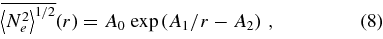
where r is given in R_s, and the three parameters A_[0,1,2] for each fit are given in Table 1, along with their respective extrapolated densities at the coronal base $\overline{N_e}$(1R_s). This near-exponential functional form corresponds to the hydrostatic equilibrium solution, being A⁻¹₂ the scale height in R_s units. Figures 11 and 12 show the radial dependence of $\overline{T}_m$ and $\overline{W}_T$, respectively, using the same symbols as in Figure 10 for each region.

Zoom In Zoom Out Reset image size

Zoom In Zoom Out Reset image size

Zoom In Zoom Out Reset image size

Table 1. Parameter Values of the Least-square Best Fits to the Estimated Electron Density as a Function of Height Given by Equation (8), Along Different Coronal Structures, and Extrapolated Density at the Coronal Base

Region	$\overline{N_e}$(1 Rs) (×108 cm−3)	A0 (×107 cm−3)	A1	A2
Streamer core center	2.39	6.44	12.76	11.45
Streamer core region of maximum $\overline{\zeta }_{195}$	2.11	6.91	10.67	9.58
Open/closed boundary	1.45	4.39	9.95	8.76
Subpolar density minimum	1.04	2.88	12.08	10.80

Download table as:  ASCIITypeset image

Table 1 and Figure 10 show that at the coronal base (1 R_s) the density in the streamer core center is the largest, gradually decreasing when moving to the higher latitude structures. Above 1.035 R_s, the densities in the streamer core center and the maximum $\overline{\zeta }_{195}$ region become comparable, with the later developing slightly larger values, as already seen in Figure 6. At all analyzed heights, the density ratio between the streamer core and the open/closed boundary ranges from 1.5 at 1.035 R_s to 1.1 at 1.195 R_s. At all heights the density ratio between the streamer core and the subpolar regions ranges from 2.1 at 1.035 R_s to 2.5 at 1.195 R_s. As already stated, these results can be affected by the inverse linear scaling of the derived electron density with the iron abundance.

Figure 11 shows that the streamer core center mean temperature is $\overline{T}_m= 1.1$ MK at the lower layers, decreases down to a minimum value of 0.95 MK at 1.115 R_s, and then it rises again up to 1.03 MK at 1.195 R_s. In the same height range, the plasma of the streamer core in the maximum $\overline{\zeta }_{195}$ region always exhibits larger $\overline{T}_m$, being 1.15 MK at 1.035 R_s, then monotonically rising up to 1.25 MK at 1.165 R_s, and maintaining that value above that height. At all analyzed heights, the plasma $\overline{T}_m$ along the open/closed boundary is only slightly smaller than in the maximum $\overline{\zeta }_{195}$ region, being of order 1.15 MK at 1.075 R_s, and reaching 1.23 MK at 1.20 R_s. Therefore, the plasma along the open/closed boundary always exhibits considerably larger $\overline{T}_m$ values with respect to the streamer core center, being 20% larger at 1.20 R_s. In the subpolar region, the plasma mean temperature is as low as $\overline{T}_m= 0.85$ MK at 1.065 R_s, and then monotonically increases, reaching similar values to those in the streamer core at 1.12 R_s. At all heights, the plasma $\overline{T}_m$ along the open/closed boundary is between 25% and 35% larger than in the subpolar regions.

Figure 12 shows that at the lower layers all four regions present a similar LDEM temperature spread $\overline{W}_T\approx 0.3$. Below 1.075 R_s, the temperature spread in the streamer core center is comparable (and even slightly larger) than along the open/closed boundary (see also Figure 9). Above that height, the open/closed boundary shows increasingly larger temperature spread compared to the streamer core center. At all heights, the values along the open/closed boundary and in the maximum $\overline{\zeta }_{195}$ region are comparable. At almost all heights the plasma along the open/closed boundary exhibits much larger temperature spread than in the subpolar region, with a contrast ratio gradually increasing with height, reaching values 300% larger at 1.1 R_s, and maintaining a comparable large contrast at higher heights.

Comparison of Figures 11 and 12, and also of Figures 8 and 9, shows that T_m and W_T are not related to each other in a simple way. There is indication of both quantities being correlated for specific small-scale structures located along polarity inversion lines, as the ARs in the northern hemisphere, for example. This is also the case of the E–W-oriented filament cavity observed in the southern hemisphere, spanning the longitudinal range [240°, 320°] and between latitudes [ − 45°, − 35°]. The underlying off-limb prominence is mapped here as the elongated enhancement on the 304 Å FBE reconstruction at 1.035 R_s in Figure 2. Above it, in matching coordinates, elongated structures of depleted 171 and 195 Å FBE values are observed, as shown at 1.075 R_s, for example, in Figure 1. Correspondingly, a density dip along the structure can be seen in the top panel of Figure 3, revealing the elongated cavity overlying the chromospheric prominence. At 1.075 R_s, the cavity center densities are of order 0.75 × 10⁸ cm⁻³ (reddish), while the surrounding streamer values are around 1 × 10⁸ cm⁻³ (green). This ∼30% density contrast is similar to the results we obtained for other filament cavities we analyzed using this same technique for another period (Vásquez et al. 2009). The middle and bottom panels of Figure 3 show that, along the cavity, the plasma presents broader and hotter LDEM distributions than in the surrounding streamer plasma. Similar results have been analyzed in detail in Vásquez et al. (2009). We postpone to another paper an extension of those detailed analyses to other cavity examples. New to this analysis is the comparison of the cavity structure to the magnetic structure. The PFSS model presents a clear polarity inversion line exactly aligned with the filament and cavity geometries in all their extension. Even if a subtle structure, not clearly visible in the EUVI image series due to projection effects, the stability of the cavity makes it an ideal candidate for tomographic analysis (see also Vásquez et al. 2009). The 3D density and temperature structure of the cavity-streamer region is thus empirically revealed for the first time without the need of an ad-hoc geometrical model for the structure under analysis. Beyond constituting an interesting solar physics result per se, the morphological consistency between the DEMT and PFSSM structures in the cavity region, serves here also as a validation for both techniques results.

We have performed a dual-spacecraft tomographic reconstruction of the solar corona during a period of minimum activity. Having used both STEREO/EUVI instruments with the spacecraft view angles separated by an average 854 during the observational period, we gathered the data to cover the required 360° of view angles in about 3/4 of a solar corona rotation. This fact, and the much reduced solar activity during the period analyzed, yielded our reconstruction with fewer coronal cells with tomographically undetermined emissivity due to coronal fast dynamics artifacts. A comparison can be made between the results of Figure 1 and those for CR-2069 reported in Frazin et al. (2009). While the image series corresponding to that period exhibit three very bright ARs near the equator, the period we analyze here exhibits two much less bright ARs at higher latitudes, and that appear to change much less during their disk transits. Consistently, the CR-2069 FBE reconstruction exhibits ZDA regions around the ARs, which are almost not present in the CR-2077 results. As a quantification, we find, for example, that at 1.075 R_s the ζ₁₉₅ reconstruction of this work presents 3 times less ZDA voxels respect to the CR-2069 results, and the reconstructed ζ₁₇₁ presents no ZDA voxels at all.

Using the reconstructed 3D emissivity in the three EUVI coronal bands, we performed an LDEM analysis at each tomographic cell. By computing the first three moments of the resulting LDEM at each cell, we built global coronal maps of mean electron density, mean electron temperature, and electron temperature spread, in the height range 1.0–1.25 R_s. Due to the optically thick nature of the image pixels around the solar disk boundary, and the finiteness of the instruments FOVs and the computational grid, the tomographic results are meaningful between heights 1.035 and 1.225 R_s. For interpretation of the tomographically derived results in terms of the corona magnetic structure, we also developed a PFSS model of the solar corona driven by MDI/SOHO magnetograms of the same period.

Regarding the large-scale density structure of the solar corona, we find (Figures 3 and 6) that the equatorial streamer core densities are at least double those in the subpolar regions, with possible gravitational settling of the Fe ions (see below) affecting the values derived for the streamer core. The latitudinal extension of the streamer core, as defined by the open/closed boundaries of the PFSS model, gradually decreases with height, being 122° at 1.035 R_s, and 98° at 1.195 R_s. In each hemisphere, the streamer/subpolar density transition latitudinal range is roughly centered in the open/closed boundary. The streamer/subpolar density latitudinal derivative gradually decreases with height, becoming less steep. Figure 7 shows that at 1.035 R_s 76% of that transition occurs over a 20° latitudinal range centered around the open/closed boundary, while the fraction goes down to 60% at 1.195 R_s.

The estimated electron density is inversely proportional to the iron abundance values used for the LDEM inversion. While in this work, this number has been assumed uniform, abundance depletion of heavier elements due to gravitational settling is usually observed in quiescent streamer cores. The issue of elemental abundance in streamers has been studied with the Ultraviolet Coronagraph Spectrometer (UVCS; Kohl et al. 1995) aboard the SOHO. Those studies cover heliocentric heights typically in the range 1.5–2.0 R_s. For quiescent streamers, UVCS studies have reported iron abundance values ranging from values 10 times lower than those used here (Raymond et al. 1997; see also Vásquez & Raymond 2005) to values of order one-half (Uzzo et al. 2007), although those studies cover larger heights than those analyzed here. At lower heights, Landi et al. (2006) have analyzed the iron abundance using observations of the Solar Ultraviolet Measurements of Emitted Radiation (SUMER) spectrometer aboard SOHO. The region they analyze corresponds to a dual-streamer structure during the rising phase right after the 1996–1997 minimum. By analyzing the emission measure derived from high and low FIP elements, they find that below 1.4 R_s that FIP bias is roughly constant and about 3.5. By analyzing the Mg x to Fe xii line ratios, they explore the degree of gravitational settling between heights 1.1 and 1.7 R_s. Their results show that iron abundance does not vary much in the height range of our analysis within their streamer regions, but it clearly differs from that part of their FOV affected by coronal hole plasmas. Still, those results correspond to a complex of streamer structure. If iron depletion variations exist at the lower heights of the more organized and larger streamer belt we analyzed, electron densities in the streamer core could be higher than those reported here. On the other hand, the signal recorded in pixels from dim regions of the EUV images is affected by a strong instrumental PSF contamination from bright nearby regions. Bearing in mind these two issues, the streamer/subpolar density contrast ratio reported here should be regarded as a lower bound to the real value. A variable iron abundance within the streamer core region, that would exhibit more depletion in the streamer core central latitudes, could also explain the local minimum in electron density reported here for that region.

The PFSS model magnetic strength contour plots, and the longitude-averaged radial magnetic flux density plots, suggest that the central latitudes of the streamer core are populated by relatively smaller scale magnetic loops, while the higher latitudes are populated by larger scale loops, with their foot-points at comparable latitudes in the opposite hemispheres. Comparison with the DEMT results indicates that the boundary between these two magnetically closed regions is characterized by enhanced EUV emissivities, and that the larger scale loops (closer to the open/closed boundary) show the highest mean electron temperature T_m, which tends to be lower in the central latitudes of the streamer core. At all longitudes, these high mean temperature regions do not extend into the magnetically open regions. Another interesting result regarding the streamer temperature structure is that, while along the open/closed boundary $\overline{T}_m$ monotonically increases with height, in its central region it has a minimum of $\overline{T}_m= 0.85$ MK at 1.115 R_s. Regarding the LDEM temperature spread $\overline{W}_T$, its values are also enhanced in the higher latitudes within the streamer closed region but, unlike $\overline{T}_m$, these broader distributions are also present in the magnetically open field regions immediately surrounding the open/closed boundary. At heights reported here, these regions, that are part of the so-called streamer legs, exhibit up to 3 times larger $\overline{W}_T$ values than the magnetically open regions at the higher subpolar latitudes.

Our results for average electron temperature and electron density can in principle be compared with those derived by Landi et al. (2006). Using SUMER data, they derived electron temperatures and densities in the low corona from SUMER data taken during 1998 April, in the early rising phase after the 1996–1997 solar minimum. Their data are representative of low- to mid-latitude quiet regions, between heights 1.1 and 1.7 R_s. From Mg x to Si xi line ratios analysis, they found electron temperatures in the range of 1.25–1.60 MK. In the height range 1.1–1.2 R_s, they obtained a fairly constant electron temperature of about 1.4 MK, while in that same height range our streamer core structure exhibits an average T_m value of order 1.15 MK, with peak values of order 1.25 MK. The differences may be partly ascribed to their study corresponding to a period of increased activity, as well as to differences in the analysis methods. The coronal structure was more complex during the period covered by their study, with the west limb dominated by a double streamer structure. That complexity, and the projection effects affecting their analysis, make a more detailed comparison to our results quite difficult. For a limited fraction of their FOV, Landi et al. (2006) also derive electron densities from Si viii doublet ratios. At 1.0 R_s they found electron densities of order 10⁸ cm^-3, and a factor of 5 smaller at 1.2 R_s. Those values compare with our streamer core results that are of order 0.8 and 0.3 ×10⁸ cm^-3 at those two heights, respectively (see Figure 10). Again, one must bear in mind that the values from Landi et al. (2006) correspond to the boundary and the core of a more complex streamer structure.

The empirical evidence accumulated over the last decades has brought a general consensus on that the source of the slow wind is the magnetically open regions surrounding the streamer core, at least during times of low magnetic activity. Two major scenarios have been proposed. In the first one, the streamer leg regions constitute the path along which the slow component of the solar wind is continuously channeled out from the coronal base, and the particular geometry of their constitutive field lines, with very large expansion factors, plays an important role in its lower terminal speed (Levine et al. 1977; Wang & Sheelev 1990; Vásquez et al. 2003). In a second scenario, the slow wind originates also at the open/closed boundary, and at the streamer cusp, as a result of reconnection and opening of the closed regions that allow material originally trapped in the streamer core to flow out, as originally observed by Wang et al. (1998; see also Wang et al. 2000; Fisk 2003). This last scenario has been argued to require the reconnecting loops to contain denser and hotter material, implying a larger mass to accelerate and therefore lower terminal speeds (Gloeckler et al. 2003).

Observational analyses support the combination of both scenarios as being responsible for the different properties of the slow solar wind. In an extensive recent observational analysis of the solar wind properties near the Heliospheric current sheet (HCS), based on Ulysses and Advanced Composition Explorer data and covering about 400 HCS crossings, Suess et al. (2009) identify two distinct regimes of the slow wind, distinguished by different He/H abundance ratios. The two regimes are interpreted by the authors as resulting of the two different generation scenarios mentioned above. One of them corresponds to a steady flow along the streamer legs from the base of the corona. By using composition data from SWICS, Suess et al. (2009) argue that this regime of the slow wind does not undergo significant mixing with the fast wind plasma that flows along the coronal holes' open magnetic field lines located adjacent to the streamer legs. If this is the case, a sharp transition of plasma properties between the slow and fast components of the solar wind could occur even at low coronal heights. The very steep W_T latitudinal gradient that we find in the magnetically open regions, a few degrees in latitude outside the open/closed boundary, may be indicative of this transition.

Beyond any interpretation, we can highlight some important results from the present analysis of the CR-2077 that covers the heights range 1.035–1.195 R_s.

• 1.  
  At longitudes corresponding to the more simply organized dipolar corona, the location of the streamer/subpolar density transition matches the PFSS magnetically open/closed boundary. The streamer/subpolar density ratio is at least 2, and about 70% of that transition occurs over a 20° latitude wide layer surrounding the open/closed boundary.
• 2.  
  Within the streamer core, the higher latitudes exhibit larger mean temperatures and broader LDEM, compared to the central part of the streamer. The higher latitudes are seemingly populated by the larger scale coronal loops with foot-points in the opposite hemispheres, while lower latitudes are populated by smaller scale loops. The boundary between the larger and smaller scale loops within the streamer core is characterized by enhanced EUV emissivity (vertical green dashed lines in Figure 4).
• 3.  
  The LDEM in the streamer core center and the open/closed boundary differ in significant ways. In the streamer core the radial dependence of the mean electron temperature develops a minimum around 1.12 R_s. In contrast, along the open/closed boundary the temperature increases monotonically with height. Also in the streamer core, the temperature spread decreases with height, while it is roughly constant along the open/closed boundary.
• 4.  
  The magnetically open region immediately surrounding the streamer core exhibits much broader LDEM distributions than the adjacent open regions at higher latitudes. This latitudinal transition is quite sharp. Between heights 1.1 and 1.2 R_s, the plasma along the magnetically open/closed regions' boundaries is 50%–100% denser than that in the subpolar regions, with a 25%–35% larger mean electron temperature, and with 250%–300% larger temperature spread.
• 5.  
  We find that, in general, T_m and W_T are not related to each other in a simple way.

This is the first detailed global corona analysis of DEMT results, in contrast to Vásquez et al. (2009), where we focused only on filament cavities. In order to draw more general conclusions, further application of the technique to other Carrington rotations is needed. We are currently performing an analysis similar to the one presented here for the Whole Heliosphere Interval (CR-2068), to investigate similarities and differences with the results of this work. We also plan to compare results from DEMT reconstructions with 3D MHD models of the solar corona, as we have already done for white light reconstructions of the 3D electron density (Vásquez et al. 2008). In particular, we plan to make comparisons against the MHD model by Manchester et al. (2008), where they make a detailed comparison between the mass density of a CME inferred from LASCO observations and the density predicted by the model. For a different CME event, we aim to improve the model predictions by specifying its boundary conditions and volumetric constraints with DEMT reconstructions. Regarding planned further development of the DEMT technique, the PSF deconvolution of the images used for tomography will improve the capability of the method to more accurately evaluate strong density gradients, allowing us to expand the analysis into the CH regions. We also plan to refine the LDEM determination through the application of Markov chain Monte Carlo methods, using the six Fe bands of the Atmospheric Imaging Assembly (AIA) on the Solar Dynamics Observatory. Finally, we also aim to eventually implement time-dependent DEMT through the application of the Kalman filtering method (Frazin et al. 2005; Butala et al. 2008).

We thank the anonymous referee for the insightful review of our manuscript, and for constructive suggestions that enriched its content in a significant way.

We thank Jean-Pierre Wuelser for his priceless assistance with the EUVI data. We thank Leonard Strachan and John C. Raymond for their valuable comments that improved the scientific content of the manuscript. This research was supported by NASA Heliophysics Guest Investigator award NNX08AJ09G to the University of Michigan, and the NSF SHINE and CMG programs, awards 0555561 and 0620550, respectively, to the University of Illinois. A.M.V. acknowledges the ANPCyT PICT/33370-234 grant to IAFE for partial support. W.B.M.IV acknowledges NASA grant number LWS NNX06AC36G.

The STEREO/SECCHI data used here are produced by an international consortium of the Naval Research Laboratory (USA), Lockheed Martin Solar and Astrophysics Lab (USA), NASA Goddard Space Flight Center (USA) Rutherford Appleton Laboratory (UK), University of Birmingham (UK), Max-Planck-Institut für Sonnensystemforschung (Germany), Centre Spatiale de Liege (Belgium), Institut d'Optique Théorique et Appliqueé (France), and Institut d'Astrophysique Spatiale (France).