


ABSTRACT
Nonlinear force-free field (NLFFF) extrapolation is a powerful tool for the modeling of the magnetic field in the solar corona. However, since the photospheric magnetic field does not in general satisfy the force-free condition, some kind of processing is required to assimilate data into the model. In this paper, we report the results of new preprocessing for the NLFFF extrapolation. Through this preprocessing, we expect to obtain magnetic field data similar to those in the chromosphere. In our preprocessing, we add a new term concerning chromospheric longitudinal fields into the optimization function proposed by Wiegelmann et al. We perform a parameter survey of six free parameters to find minimum force- and torque-freeness with the simulated-annealing method. Analyzed data are a photospheric vector magnetogram of AR 10953 observed with the Hinode spectropolarimeter and a chromospheric longitudinal magnetogram observed with SOLIS spectropolarimeter. It is found that some preprocessed fields show the smallest force- and torque-freeness and are very similar to the chromospheric longitudinal fields. On the other hand, other preprocessed fields show noisy maps, although the force- and torque-freeness are of the same order. By analyzing preprocessed noisy maps in the wave number space, we found that small and large wave number components balance out on the force-free index. We also discuss our iteration limit of the simulated-annealing method and magnetic structure broadening in the chromosphere.
Export citation and abstract BibTeX RIS
1. INTRODUCTION
Coronal field extrapolation is one of the main subjects in solar physics. This is because many solar active phenomena in which we are interested happen in coronal magnetic fields. Our purpose in this study is to improve the bottom boundary of nonlinear force-free field (NLFFF) extrapolation. This is called preprocessing (Wiegelmann et al. 2006). Here we give a brief introduction on this subject.
Direct observation of coronal magnetic fields is presently difficult. One reason is the low brightness of coronal emission lines, and another reason is inversion of the three-dimensional structure of coronal fields from two-dimensional data. As far as we know, only one paper on a spectropolarimetry observation of a coronal emission line has been published (Lin et al. 2004). They obtained full Stokes profiles of limb coronal fields and found that field strength is about 4 G at 100'' in height above the photosphere. One of the main purposes of the Advanced Technology Solar Telescope (ATST) is to observe coronal magnetic fields (see Keil et al. 2004 and their Web site2).
Because of these difficulties in observation, scientists have tried so far to obtain coronal field structures by solving the boundary value problem with magnetic field data on the photosphere. Recently, benchmarks of various NLFFF extrapolation methods were carried out (Schrijver et al. 2006; Metcalf et al. 2008; De Rosa et al. 2009). For precise descriptions of the NLFFF extrapolation methods, see these papers and references therein. These papers reported that NLFFFs calculated by various methods are inconsistent in solar active regions.
De Rosa et al. (2009) calculated about 60 NLFFF models from magnetic field data on AR 10953, and compared 12 of them with three-dimensional loops obtained by stereoscopic reconstruction from STEREO/SECCHI EUV images (Howard et al. 2008). They investigated differences between these NLFFFs and pointed out difficulties in the entire NLFFF extrapolation process, including 180° ambiguity solvers and preprocessing methods, from magnetic fields in the photosphere. One of the difficulties is that magnetic fields in the photosphere are perturbed by various forces (e.g., pressure gradient forces). This difficulty is the main motivation for preprocessing.
The NLFFF methods extrapolate coronal fields from observed magnetic field data, considering coronal magnetic fields as NLFFFs, namely J × B = 0. However, as we described above, one problem arises in the extrapolation because plasma β is more than unity on the photosphere, while in the corona plasma β is less than unity. There are three possible solutions for this problem:
- 1.solving the magnetohydrodynamic equilibrium including the magnetic force, gas pressure, and gravity (namely, J × B − ∇P + ρg = 0);
- 2.adopting vector magnetograms in the chromosphere as the bottom boundary condition; or
- 3.preprocessing vector magnetograms observed on the photosphere.
Regarding the first solution, nothing can solve the force-free equation including the gas pressure and gravity with the observed vector magnetogram at present. In order to solve this equation, we should understand quantitative relations between the temperature, number density, and magnetic field in the corona. We need to clarify the coronal heating and cooling process.
Regarding the second solution, solar physicists try to obtain vector magnetograms in the chromosphere. In some observatories, instruments for full Stokes observation in chromospheric lines have been developed. Some solar physicists study the polarization process and try to obtain magnetic fields from full Stokes data (e.g., Lagg et al. 2004; Asensio Ramos et al. 2008). At present, however, it is more difficult to obtain vector magnetograms in the chromosphere than in the photosphere.
In this paper, we study preprocessing of vector magnetograms. Wiegelmann et al. (2006) first suggested preprocessing vector magnetograms for NLFFF extrapolations. The main purpose of preprocessing is to improve vector magnetograms as force- and torque-free fields. For this purpose, Wiegelmann et al. (2006) developed a method to decrease indices of force- and torque-freeness in a vector magnetogram by solving a minimum value problem of their function with the Newton-Raphson method.
Later, Fuhrmann et al. (2007) suggested another way of preprocessing by solving their optimization function with the simulated-annealing method. In Fuhrmann et al. (2011), Wiegelmann's and Fuhrmann's methods are compared. By their methods, indices of force- and torque-freeness of a vector magnetogram decreased at least by 104. However, as shown in Table 1 of Fuhrmann et al. (2011), there are no significant improvements of several indices in NLFFFs extrapolated with preprocessed fields (e.g., average values of |J × B|).
Referring to these previous results, one of our objectives is to using longitudinal magnetograms in the chromosphere. This is because magnetic fields in the chromosphere are a more appropriate boundary condition for NLFFF extrapolation than are those in the photosphere. Another objective is to find the best parameters for our preprocessing method. In this study, we apply the simulated-annealing method and a function including the magnetic field of the chromosphere. We need to investigate the distribution of preprocessed results in parameter regions.
In Section 2, we describe our method and data. In Section 3, we show the results of the parameter survey. In Section 4, we discuss the limitation of our method. Conclusions are briefly summarized in Section 5.
2. METHOD AND DATA
In Section 2.1, we introduce preprocessing. In Section 2.2, we describe the simulated-annealing method. In Section 2.3, we describe our data set.
2.1. Preprocessing
Wiegelmann et al. (2006) first proposed preprocessing magnetic field data. In order to quantitatively perform preprocessing, they applied a function (L) as follows:


where μ1 to μ4 are coefficients of L1 to L4, respectively; L1 is the square of the total magnetic force; L2 is the square of the total magnetic torque; L3 is the difference between the preprocessed magnetogram and the observed one; L4 is the amount of small-scale irregularities in the magnetogram; and the superscript "obs" indicates the observed magnetic field.
Here, L1 and L2 come from area integrals of the Lorentz force on a volume (Wiegelmann et al. 2006). In the following, we describe derivations of the area integrals (Fuhrmann et al. 2007). If J × B =0 in a volume (V), a volume integral of the Lorentz force is equal to zero, and we can obtain the following derivation using Gaussian's theorem:


where S is the entire closed surface on the volume and T is magnetic stress tensor,
As for a volume integral of the torque, we can also perform a similar derivation:

In preprocessing, we consider this closed surface to be six surfaces of a computational cube. If the contributions of the side and top boundaries of the cube are small, one integrates only over the bottom boundary. Finally, the following equations are derived:
In the solar atmosphere, this bottom boundary corresponds to the photosphere or to the chromosphere. Note that this is reasonable for an isolated and flux-balanced active region. Using these equations, we can expect that lower values of L1 and L2 indicate better degrees of force- and torque-freeness of magnetic fields. For original derivations of the area integrals, see Molodenskii (1969) and Aly (1989).
L3 is a parameter to obtain preprocessed magnetic fields similar to the observed fields. L4 is a parameter controlling the smoothness of magnetic fields. These parameters are independent of L1 and L2 and control the appearance of magnetic fields. We will discuss how combinations of μ1 to μ4 control preprocessing.
In this study, we add a term into the function as follows:

where Bchrz is the longitudinal magnetic field in the chromosphere and μ5 is a coefficient. In this study, we use a longitudinal magnetogram observed by SOLIS. We will describe these data later.
Note that, in our function, free parameters are μ3 to μ5. μ1 and μ2 are constants in this study. μ1 is set to be 10. μ2 is determined by μ1 as follows (Wiegelmann et al. 2006):

where D is the pixel size of our data. In this paper, D is 256.
2.2. How to Obtain Minimum Values
In previous studies, Wiegelmann et al. (2006) used the Newton-Raphson method to obtain local minima, and Fuhrmann et al. (2007) used the simulated-annealing method. For precise descriptions of these methods, see Press et al. (1992). In this study, in order to obtain minima, we apply the simulated-annealing method. One reason why we apply this method is that the simulated-annealing method provides the opportunity to obtain minimum values far from the initial conditions. On the other hand, the Newton-Raphson method obtains local minimum values near the initial condition.
The simulated-annealing method assumes the pseudo-temperature (T) and its cooling rate (dT) of the system. T decreases step by step as Tnew = T × dT. In this method, perturbation of the magnetic field is given by random numbers on each pixel. Concerning variations of L, a decrease of L is always allowed. On the other hand, an increase of L is allowed if a random number is smaller than the probability (P). P is defined as P = exp (− dL/T), where dL is the variation of L derived from perturbed magnetic fields. If T is much lower, L hardly increases in calculations. In other words, if T is higher, L can increase, and we can find minimum values far from the initial conditions.
In our calculations, the initial value of T is defined as Tinit = t0L0, where t0 is the initial temperature coefficient and L0 is the initial value of L. In addition to t0 and dT, the seed of the random numbers is also a free parameter. Including μ3, μ4, and μ5, we perform a parameter survey of these six parameters.
We finish our calculations when values of L converge or pseudo-temperatures T achieve the threshold temperature. Convergence of L is reached when variations of L, |Lnew − Lold|/(Lnew + Lold), are less than 10−6 through five steps. The threshold temperature (Tstop) is set to be Tstop = Tinit10−100. Therefore, we can obtain enough steps for the temperature cooling. If pseudo-temperature T achieves Tstop, we consider the results to be non-converging.
2.3. Data
In this study, the target region is AR 10953. We analyze a vector magnetogram on the photosphere and a longitudinal magnetogram in the chromosphere. The vector magnetogram is observed by the Hinode/Solar Optical Telescope (SOT; Kosugi et al. 2007; Tsuneta et al. 2008; Suematsu et al. 2008; Ichimoto et al. 2008; Shimizu et al. 2008), and the longitudinal magnetogram is observed by the SOLIS/Vector Spectro Magnetograph (VSM; Jones et al. 2002). These data are observed around 18:00 UT on 2007 May 2. The top panels of Figure 1 show magnetic field components observed by Hinode/SOT. Figure 2 shows longitudinal fields observed by SOLIS/VSM.

Figure 1. Magnetic field maps of AR 10953. Top panels show magnetic fields observed by Hinode/SOT. Bottom panels show preprocessed magnetic fields (parameter number 63). Red and blue indicate positive and negative polarities, respectively. The dynamic range of display is within ±3000 G.
Download figure:
Standard image High-resolution image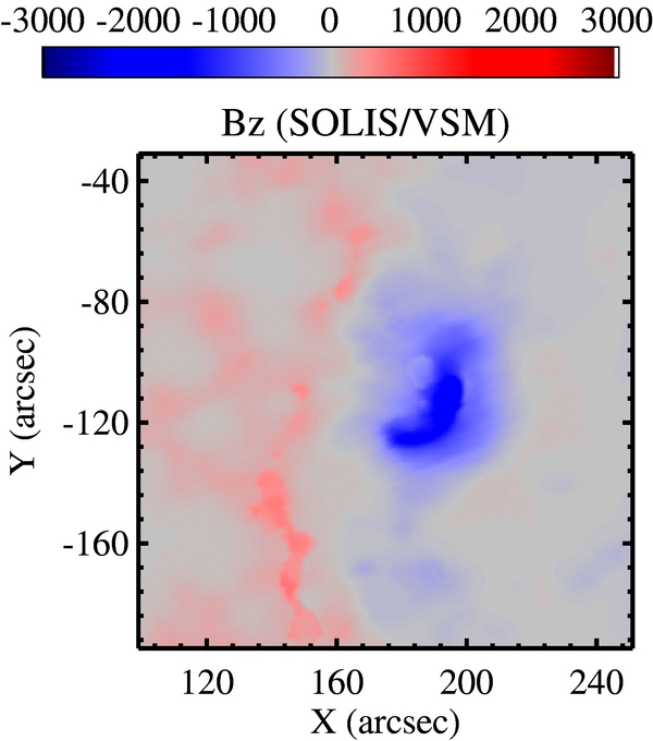
Figure 2. Magnetic field maps of AR 10953 observed by SOLIS/VSM. Red and blue indicate positive and negative polarities, respectively. The dynamic range of display is within ±3000 G.
Download figure:
Standard image High-resolution imageThe vector magnetogram is SOT/SP level 2 data ("20070502_173005.fits"). This file can be downloaded from the LMSAL Web site.3 These level 2 data are inverted with the MERLIN code from full Stokes data observed in the Fe i λ6301.5 and λ6302.5 lines. To solve the 180° ambiguity of transverse field azimuth, we apply the minimum energy method (for more precise information, see Leka et al. 2009 and their Web site4).
The longitudinal magnetogram in the chromosphere is observed in Ca ii 8542 Å line. The file name is "svsm_m2100_S2_20070502_1832.fts." This file can be found on the NSO Web site.5
Magnetic field data are interpolated to have a number of pixels, 256 × 256. The original number of pixels in the vector magnetogram is 512 × 512. Pixel widths are set to be about 0.6 arcsec. Alignment of coordinates between the vector magnetogram and the longitudinal magnetogram is calculated from weighted centers of longitudinal fields.
3. RESULTS
We perform a parameter survey on six free parameters: the initial temperature coefficient (t0), the temperature cooling rate (dT), and the seed of the random numbers, μ3, μ4, and μ5. In this survey, we perform calculations with 86 combinations of these free parameters. These 86 combinations are listed in the electronic edition with examples of parameter combinations listed in Table 1. In Section 3.1, we describe preprocessed maps whose force-freeness is smaller. In Section 3.2, we explain our parameter survey. In Section 3.3, we describe contributions of large and small wave number components to force-freeness.
Table 1. Examples of Free Parameter Combinations
| No.a | log(t0) | dT | log(μ3) | log(μ4) | log(μ5) | Seedb | Cnv.c | r1 | r5 |
|---|---|---|---|---|---|---|---|---|---|
| 0 | −4 | 0.9950 | 7 | 7 | 7 | 3 | 1 | 1.385e+07 | 1.252e+02 |
| 1 | −4 | 0.9950 | 8 | 7 | 7 | 3 | 1 | 6.166e+05 | 1.103e+01 |
| 2 | −4 | 0.9950 | 7 | 8 | 7 | 3 | 1 | 4.560e+06 | 3.793e+01 |
| 3 | −4 | 0.9950 | 7 | 7 | 8 | 3 | 1 | 1.194e+07 | 1.805e+03 |
| 4 | −4 | 0.9995 | 7 | 7 | 7 | 3 | 1 | 2.593e+07 | 2.857e+02 |
Notes. aParameter combination number. bRandom number seed. cCalculation convergence code; 1 = converged.
Only a portion of this table is shown here to demonstrate its form and content. A machine-readable version of the full table is available.
Download table as: DataTypeset image
3.1. Preprocessed Maps
Figure 3 shows a scatter plot of the parameter combinations. r1 and r5 are ratios (initial values/final values) of L1 and L5, respectively. These values are summarized in the online version of Table 1. In this figure, larger values of r1 indicate magnetic fields closer to force free, and those of r5 indicate longitudinal fields closer to the chromospheric field. Therefore, larger values in both r1 and r5 indicate more ideal boundary conditions of NLFFF extrapolations.
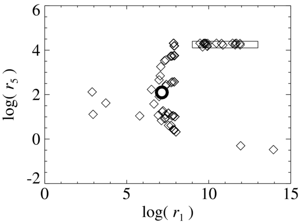
Figure 3. Scatter plot of the parameter survey. The x- and y-axes show variation amplitudes of L1 and L5, respectively. The open circle around the center shows parameter number 0. The rectangle in this plot shows the plot range of Figure 4. These values are summarized in the online version Table 1.
Download figure:
Standard image High-resolution imageFigure 4 shows an enlarged view of the rectangle region in Figure 3. In this figure, numbers in gray show non-converging results. This non-converging indicates L did not converge within iteration limits. In our calculation, maximum iteration limits depend on t0 and dT. We discuss these iteration limits in a later section.
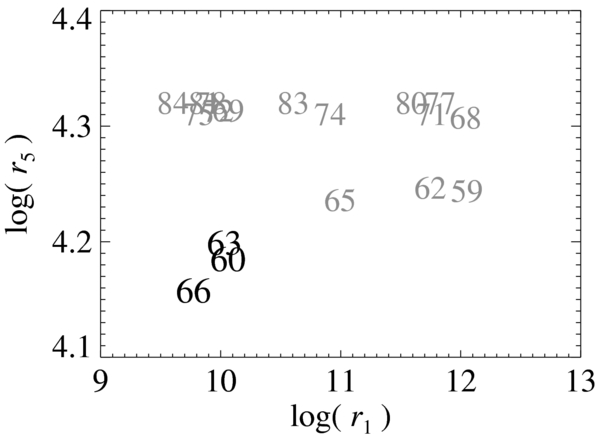
Figure 4. Scatter plot of parameter combinations. The x- and y-axes show variation amplitudes of L1 and L5, respectively. Numeric characters in gray and black indicate parameters of non-convergence and convergence, respectively.
Download figure:
Standard image High-resolution imageAs a result, Figure 4 shows that parameter numbers 60, 63, and 66 show the largest values of r1 and r5. μ4 is the difference between these parameter combinations (μ4 = 103 for 60, 104 for 63, and 105 for 66). The bottom panels of Figure 1 show preprocessed magnetic field maps of parameter number 63. Figure 5 shows variations of the function. In the following, we describe differences in the preprocessed field strengths of these parameter combinations. Magnetic field maps of these parameter combinations are similar to each other.
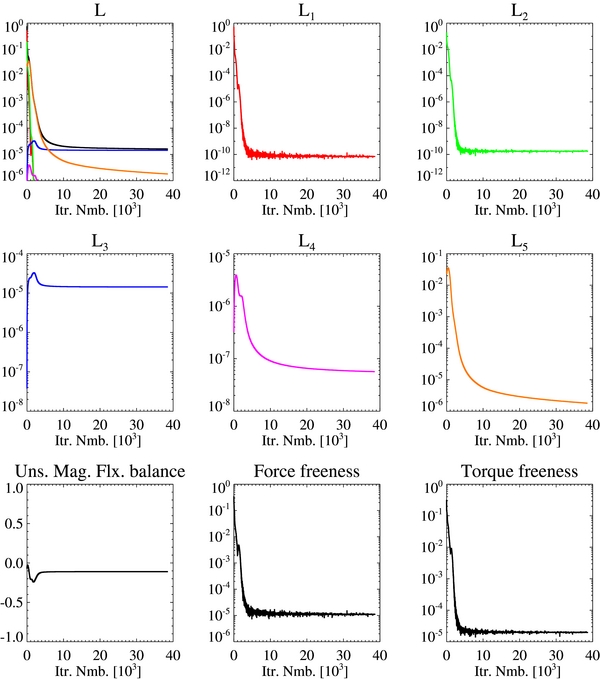
Figure 5. Evolutions of terms of the function (L1–L5), the magnetic flux balance, the force freeness, and the torque freeness in the case of parameter number 63.
Download figure:
Standard image High-resolution imageThe bottom panels of Figure 1 show that the preprocessed map of Bz is very similar to the longitudinal fields shown in Figure 2. It is found that, in 98% of the pixels, unsigned differences of Bchrz − Bz63 are lower than 5 G, where superscript 63 shows the parameter number. More precisely, the standard deviation of Bchrz − Bz63 is 1.9 G. As for parameter numbers 60 and 66, standard deviations of B63z − Bzi (i = 60 and 66) are 0.1 and 0.2 G, respectively.
Figure 6 shows histograms of B63t − Bt60, where Bt = (B2x + B2y)0.5. This figure shows that 90% of all pixels have unsigned differences of Bt less than 15 G. In pixels where |B63z| is larger than 1000 G (a black area in the negative polarity in the bottom right panel of Figure 1), 50% of the pixels have unsigned differences of Bt less than 15 G. Between parameter numbers 63 and 66, 76% of all pixels have unsigned differences of Bt less than 15 G. In pixels where |B63z| is larger than 1000 G, 29% of pixels have unsigned differences of Bt less than 15 G.
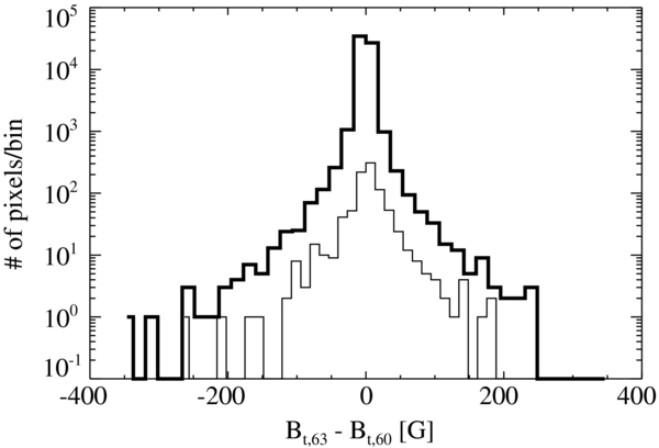
Figure 6. Histogram of B63t − Bt60 (the thick line). The thin line shows the histogram where |B63z| is greater than 1000 G.
Download figure:
Standard image High-resolution imageFor comparison, here we describe results of parameter number 11. This parameter combination lies at the bottom right end of Figure 3 and shows the largest r1 (namely the smallest L1). In this parameter combination, only coefficients of force- and torque-freeness are emphasized. Figures 7 and 8 show preprocessed field maps and profiles of the function. As shown in Figure 7, the resultant fields are very noisy. What is important in this figure is the possibility that noise fields are candidates of local minimum values. This will be discussed in a later section.

Figure 7. Magnetic field maps of preprocessed magnetic fields (parameter number 11). Red and blue indicate positive and negative polarities, respectively. The dynamic range of display is within ±3000 G. White and black show regions where field strengths are larger than +3000 G and smaller than −3000, respectively.
Download figure:
Standard image High-resolution image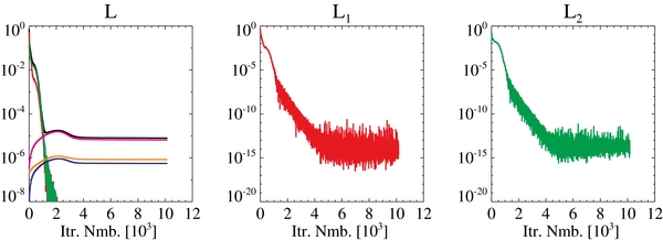
Figure 8. Evolutions of the functions L1 and L2 of parameter number 11.
Download figure:
Standard image High-resolution image3.2. Parameter Survey
Figure 3 is the scatter plot of all parameter combinations. The open circle in this figure shows the standard parameter combination (parameter number 0). As the first step, we irregularly change free parameters. These are parameter numbers 1–14. From these parameter combinations, we find that the initial temperature factor and the seed of random numbers have minor effects on calculation results.
Second, we check variations of temperature cooling rate (dT), μ4, and μ5 in parameter numbers 0, 2–4, and 15–58. Parameters are dT = [0.995, 0.999, 0.9995], μ4, and μ5 = [105, 106, 107, 108]. Figure 9 shows a scatter plot of these parameter combinations. This figure shows a clear dependence of r5 on μ5. Parameter combinations of μ5 = 108 show larger values of r5, which means that parameter combinations of μ5 = 108 are more favorable than the other parameter combinations. Figure 10 is a scatter plot of μ5 = 108. Table 2 shows dT and μ4 of the parameter combinations shown in Figure 10. From Figure 10 and Table 2, the following two points are found: (1) lower μ4 and larger dT lead to larger r1; and (2) in lower μ4, cooling rates (dT) result in smaller differences in r1. Hereafter, we consider only one cooling rate, 0.995.
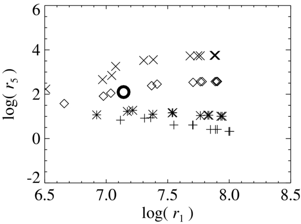
Figure 9. Scatter plot of parameter numbers 0, 2–4, and 15–58. "+," "*," " ," and "×" indicate μ5 = 105, 106, 107, and 108, respectively. The open circle shows parameter number 0.
Download figure:
Standard image High-resolution image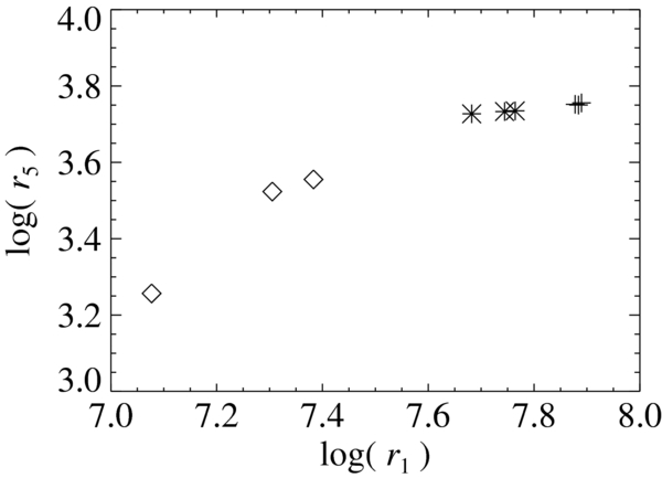
Figure 10. Scatter plot of parameter combinations of μ5 = 108 shown in Figure 9. "+," "*," and " " indicate μ4 = 105, 106, and 107, respectively.
Download figure:
Standard image High-resolution imageTable 2. Parameter Combinations Shown in Figure 10
| No. | dT | log(μ4) | log(r1) | |
|---|---|---|---|---|
 |
3 | 0.995 | 7 | 7.08 |
| 47 | 0.999 | 7 | 7.31 | |
| 31 | 0.9995 | 7 | 7.38 | |
| * | 18 | 0.995 | 6 | 7.68 |
| 49 | 0.999 | 6 | 7.74 | |
| 33 | 0.9995 | 6 | 7.76 | |
| + | 19 | 0.995 | 5 | 7.89 |
| 50 | 0.999 | 5 | 7.88 | |
| 34 | 0.9995 | 5 | 7.88 |
Download table as: ASCIITypeset image
As the third step, we check variations of μ3, μ4, and μ5 in parameter numbers 59–85. In these parameter combinations, parameters are set as follows: μ3 = [105, 106, 107], μ4 = [103, 104, 105], and μ5 = [108, 109, 1010]. As shown in Figure 4, calculations of some parameter combinations converge, while others do not. Therefore, positions of parameter combinations in Figure 4 strongly depend on μ3 and μ5. In the right side of log(r1) = 10.3, μ3 is 105. In the left side, μ3 is 106. In the upper part of log(r5) = 4.25, μ5 is 109 and 1010. In the lower part, μ5 is 108. As described in the previous subsection, μ4 of parameter numbers 60, 63, and 66 are 103, 104, and 105, respectively.
Finally, concerning parameter number 63, we change dT, t0, and the seed of the random numbers: dT = [0.995, 0.999, 0.9995], t0 = [10−4, 10−1, 1]. From these calculations, values of log(r1) are distributed from 9.86 to 9.90, and those of log(r5) are distributed from 4.167 to 4.194. In these calculations, dT and t0 determine r1 and r5, although the ranges of r1 and r5 are small. Seeds of random numbers have minor effects on these results.
We find in the third step that, if μ5/μ3 is greater than 102, the calculations do not converge. As for parameter numbers 60, 63, and 66, values of μ5/μ3 are 102. As for the other parameter combinations shown in Figure 4, values of μ5/μ3 are equal to or larger than 103. We will discuss non-converging parameters in a later section.
3.3. In the Wave Number Space
In Section 3.1, we point out that noisy maps can take smaller force- and torque-freeness, namely smaller L1 and L2, in preprocessing. Here, we quantitatively investigate this tendency of L1 in the wave number space from three magnetic field maps: one is the original vector magnetogram (the top panels of Figure 1), one is the preprocessed map of parameter number 63 (the bottom panels of Figure 1), and another is the noisy map of parameter number 11 (Figure 7).
In order to investigate L1 in the wave number space, we calculate values in the wave number space via Fourier transform as follows:
where  is the field strength in the wave number space, E(m, n) indicates exp (2πi[mx/Nx + ny/Ny]), and m and n are integer numbers (m ⩽ |Nx/2| and n ⩽ |Ny/2|). For precise derivation, see the Appendix.
In the following, we compare summations of Fa, Fb, and Fc in four wave number regions. The powers of four wave number regions are defined as p1 to p4 and are shown in Table 3. Four wave number regions are defined in Table 4. p0 is the total value of p1 to p4. In Table 3, p1 to p4 of the original vector magnetogram shows the single sign (either positive or negative), and p1 indicates that the small wave number component is larger than the other values. On the other hand, p1–p4 of the preprocessed magnetograms show both positive and negative signs, and p1 is not necessarily larger than the other values. As for the preprocessed maps, unsigned values of p0 of parameter number 11 are smaller than those of parameter number 63, while unsigned values of p1–p4 of parameter number 11 are larger than those of parameter number 63. Therefore, in these preprocessed magnetograms, total values of the large wave number components cancel out those of the small wave number components. This tendency is emphasized in the noisy magnetogram (parameter number 11). In Figure 7, noise (namely large wave number components) destructs the magnetic field structures and seem to develop only for decreasing L1 (canceling p1 and p4) in this preprocessing.
Table 3. Total Values of Terms of L1
| No. | p0 | p1 | p2 | p3 | p4 | |
|---|---|---|---|---|---|---|
| ∑Fa | org | 2.52e+4 | 2.42e+4 | 4.08e+2 | 5.38e+2 | 1.01e+2 |
| 63 | 3.97e−1 | 9.02e−1 | −1.88e+0 | 1.53e+0 | −1.55e−1 | |
| 11 | 4.65e−3 | 2.64e+3 | −9.77e+2 | −1.59e+3 | −6.68e+1 | |
| ∑Fb | org | −1.40e+4 | −1.34e+4 | −2.64e+2 | −2.67e+2 | −5.62e+1 |
| 63 | −3.47e−1 | 3.25e−1 | 2.19e+0 | −3.06e+0 | 1.97e−1 | |
| 11 | −9.87e−4 | 6.32e+2 | −2.36e+2 | −4.94e+2 | 9.91e+1 | |
| ∑Fc | org | −5.63e+4 | −5.14e+4 | −2.08e+3 | −2.34e+3 | −4.98e+2 |
| 63 | −4.91e−1 | −1.36e+3 | 5.47e+2 | 6.10e+2 | 2.01e+2 | |
| 11 | 4.46e−3 | 3.57e+4 | −1.08e+4 | −1.49e+4 | −1.01e+4 |
Notes. In the second column, "org" indicates the original vector magnetogram, and "11" and "63" are parameter numbers. p1 to p4 are sub-area integrated values, and p0 = ∑pi.
Download table as: ASCIITypeset image


From these results, we conclude the ideal goals of preprocessing as follows: (1) values of p1–p4 in a preprocessed magnetogram have a single sign; (2) p1 is larger than the other values; and (3) values of p1–p4 are smaller than those in an original vector magnetogram. One cause of the noisy map is clearly perturbations given to magnetic fields in the simulated-annealing method. How to give perturbations is one of our future subjects.
4. DISCUSSIONS
In Section 4.1, we discuss our iteration limit of the simulated-annealing method. In Section 4.2, we discuss broadening of magnetic structures in the chromosphere, which should be considered in an improved preprocessing method. In Section 4.3, we discuss another term describing directions of Bx and By in the chromosphere.
4.1. Iteration Limits
In this study, we limit iteration steps for calculation times. Iteration step limits are set by T and strongly depend on t0 and dT. In the non-converging parameter combinations shown in Figure 4, these limits are about 4.6 × 10⁴ steps. In order to check converging results of these parameter combinations, we perform calculations of three parameter combinations until convergence. Three parameter combinations are 59, 68, and 77, and are shown at the right end in Figure 4.
Calculations of parameter number 59 and 68 converge in 8.3 × 10⁴ and 1.4 × 10⁵ steps, respectively. Concerning parameter number 77, calculation does not converge even in one week. Resultant maps of Bz of parameter numbers 59 and 68 are very similar to Figure 7. However, as for Bx and By, there are noisy regions similar to noisy preprocessed maps of parameter number 11 (Figure 7). Excluding log (r5) of parameter number 68, log (r1) and log (r5) of parameter numbers 59 and 68 are similar values, shown in Figure 4. log (r5) of parameter number 68 becomes 4.56.
From these results and the results described in Section 3.2, we conclude that a larger μ5/μ3 ratio in parameter numbers 59–85 leads to noisy maps, especially in Bx and By. The threshold ratio is μ5/μ3 = 102. In these cases, μ3 is relatively so small that preprocessed Bx and By could end up far from the original ones shown in the top panels of Figure 1.
4.2. Magnetic Structure Broadening in the Chromosphere
Magnetic structures broadening in the chromosphere are a necessary goal of improved preprocessing methods. For example, the upper right panel of Figure 1 shows Bz in the photosphere, and Figure 2 shows it in the chromosphere. Typical spatial scales in these magnetic structures are clearly different. Therefore, one of our subjects of preprocessing is how to broaden photospheric magnetic structures. For this subject, what we need to know is how magnetic structures broaden in the chromosphere.
Here, we smoothed Bz of the photosphere and calculated correlations between this smoothed Bz and Bz of the chromosphere. Bz of the photosphere is smoothed by the Gaussian function as follows:

where G is the two-dimensional Gaussian function. We changed 1σ of the Gaussian function from 1 to 21 pixels. Figure 11 shows these correlations. In this figure, we find that correlations take large values around 5–7 pixels. The width of six pixels is about 3.6 arcsec.

Figure 11. Correlation coefficients with various sizes of 1σ of the Gaussian function. " " and "*" indicate the correlation coefficient and Spearman's rank correlation, respectively.
Download figure:
Standard image High-resolution image
This magnetic structure broadening of 3.6 arcsec should be included in our future preprocessing method. One idea is to set broadening perturbations from this length, and another idea is to include this length as the L4 term that decides smoothness of a preprocessed map. We also need to investigate magnetic structure broadening in other active regions.
4.3. Another Term from Hα Observation
One of the ideas to improve preprocessing methods is to add other pieces of information from the chromosphere. In addition to L1 to L4 terms, Wiegelmann et al. (2008) propose an additional term measuring differences of directions between chromospheric fibrils and transverse fields (Bx and By). Directions of fibrils can be measured from observed Hα images. Minimizing this additional term, we can obtain expected directions of Bx and By in the chromosphere. Wiegelmann et al. (2008) show results of preprocessing including this term and results of NLFFFs extrapolated with preprocessed magnetic fields. Preprocessing including this additional term shows better results than preprocessing without the additional term. It would be promising to add both our and Wiegelmann's additional terms into Equation (1). Multi-wavelength observations including Hα observation would be useful in deciding directions of magnetic fields. Other additional information from the chromosphere could further improve preprocessing.
5. SUMMARY
In this study, we add a new term concerning longitudinal fields in the chromosphere into the function proposed by Wiegelmann et al. (2006). By this term, a preprocessed vector magnetogram is expected to become a more appropriate boundary condition of NLFFF extrapolation than vector magnetograms in the photosphere. We perform a parameter survey with the simulated-annealing method in order to obtain the most appropriate preprocessed result within the limited iteration steps. As a result, we find some parameter combinations in which force- and torque-freeness of the preprocessed vector magnetogram are improved by ∼104. On the simulated-annealing method, t0, dT, and seeds of random numbers would have smaller effects on results than would μ3, μ4, and μ5.
Noise in preprocessed magnetograms is also discussed. In some cases, noise performs an important role in decreasing force- and torque-freenesses. However, noise should be removed in the bottom boundary condition of NLFFFs. Further investigation is needed to remove noise from preprocessed magnetograms.
We are grateful to the anonymous referee for useful comments. Fruitful discussion with S. Inoue is acknowledged. This work was supported by the GEMSIS project of the Solar-Terrestrial Environment Laboratory, Nagoya University. Hinode is a Japanese mission developed and launched by ISAS/JAXA, collaborating with NAOJ as a domestic partner and NASA and STFC (UK) as international partners. Scientific operation of the Hinode mission is conducted by the Hinode science team organized at ISAS/JAXA. This team mainly consists of scientists from institutes in the partner countries. Support for the post-launch operation is provided by JAXA and NAOJ (Japan), STFC (U.K.), NASA, ESA, and NSC (Norway). SOLIS data used here are produced cooperatively by NSF/NSO and NASA/LWS.
Facilities: Hinode - Hinode (Solar-B), SOLIS - Synoptic Optical Long Term Investigations of the Sun
APPENDIX: EQUATIONS IN THE WAVE NUMBER SPACE
Here we show derivations of the equations shown in Section 3.3. Derivations via Fourier transform are as follows:


where  is the field strength in the wave number space, E(m, n) indicates exp (2πi[mx/Nx + ny/Ny]), and m and n are the integer numbers (m ⩽ |Nx/2| and n ⩽ |Ny/2|).
Note that, from Equation (A3) to Equation (A4), terms only concerning m + m' = 0 and n + n' = 0 are left. Summation of the other terms becomes zero.
Footnotes
- 2
- 3
- 4
- 5