


ABSTRACT
This work is devoted to the construction of a data-driven model for the study of the dynamic evolution of the global corona that can respond continuously to the changing of the photospheric magnetic field. The data-driven model consists of a surface flux transport (SFT) model and a global three-dimensional (3D) magnetohydrodynamic (MHD) coronal model. The SFT model is employed to produce the global time-varying and self-consistent synchronic snapshots of the photospheric magnetic field as the input to drive our 3D numerical global coronal AMR–CESE–MHD model on an overset grid of Yin–Yang overlapping structure. The SFT model and the 3D global coronal model are coupled through the boundary condition of the projected characteristic method. Numerical results of the coronal evolution from 1996 September 4 to October 29 provide a good comparison with multiply observed coronal images.
Export citation and abstract BibTeX RIS
1. INTRODUCTION
Observations show that the magnetic field on the solar photosphere changes continuously due to magnetic emergence, cancellation, transport, and dispersal by surface motions such as differential rotation and meridional circulation. Although direct measurement of the coronal magnetic field is not possible, it is generally accepted that this three-dimensional (3D) field is evolving in response to or driven by the evolution of the photospheric field (e.g., Mackay & van Ballegooijen 2006; Yeates et al. 2007, 2008; Wu et al. 2009; Wang et al. 2011). Thus the solar corona also changes dynamically with diverse processes including the interaction of newly emerging structures with the pre-existing field, twisting and shearing of the magnetic field arcades, and magnetic reconnection. It is commonly believed that these processes can drive the field away from the potential or the force-free equilibrium, and may trigger solar eruptions such as flares and coronal mass ejections (Priest 1987; Priest & Forbes 2002; Aschwanden 2004).
Magnetohydrodynamic (MHD) theory is the simplest self-consistent model describing the macroscopic behavior of dynamic coronal evolution. Even an idealized MHD model can provide insight into the complex dynamics in the corona. Most of the existing MHD models of the global solar corona and solar wind using synoptic maps of the observed photospheric magnetic field as input are used to obtain the quasi-steady solutions (Linker et al. 1999; Feng et al. 2007, 2010; Hayashi 2005; Cohen et al. 2007, 2008; Nakamizo et al. 2009). Taking the synchronic frame of the photospheric magnetic field (Zhao et al. 1999) as the bottom boundary, a steady state of the corona has been achieved by using the relaxation method with the potential field and Parker solar-wind solution as the initial values (Hayashi et al. 2008). Besides the solar photospheric magnetic field, other data on the solar surface used to prescribe the bottom boundary conditions in the MHD simulations include the temperature map derived from the multiwavelength observation by the EUV Imaging Telescope (EIT) on SOHO (Hayashi et al. 2006), the electron density and temperature from the differential emission measure tomography (DEMT; van der Holst et al. 2010), and the transverse velocity from helioseismology (Wang et al. 2011). The global distribution for the coronal plasma and magnetic field near 2.5 RS by numerically solving a simplified self-consistent one-dimensional MHD system has been employed to prescribe the coronal plasma parameters and magnetic field on the bottom boundary (Shen et al. 2010, 2011a, 2011b) in order to achieve a realistic ambient solar wind for studying coronal mass ejections. Recently, Hayashi (2012) incorporated the observation of the interplanetary scintillation into determining the conditions of the bottom boundary at 50 solar radii. Such an MHD equilibrium is treated as the reconstructed corona and solar wind, representing a time-average structure or a given state of the corona. Since the evolution of the large-scale corona can be neglected in short timescales of a few hours or days, i.e., much less than a solar rotation period, steady reconstruction of the corona is usually used for modeling the temporary background of transient events. However, the dynamic evolution of the global corona for several months is significantly controlled by the bottom magnetic field changes (Zhao et al. 1999). Time sequences of successive coronal equilibria are trying to keep pace with the time-varying evolution by patching those based on the corresponding synoptic frame of each time, although these coronal steady states cannot change synchronously with the real evolution of the global photospheric magnetic field.
To further follow the time evolution of the global corona, a dynamic model is required. To date, several models exist that aim to depict the dynamic evolution of the corona using observed data as input, e.g., the data-driven MHD model for active-region evolution by Wu et al. (2006), the coupled models for the corona and the emergence flux in the active region by Abbett et al. (2004). All of these models, however, are designed for the local corona, mainly the active regions, with short timescale of minutes or hours. For long-term variation, Mikić et al. (1999) studied the quasi-steady evolution of the large-scale coronal structure using a sequence of synoptic Kitt Peak National Observatory synoptic magnetic maps as input at the bottom boundary to drive their corona model. Lionello et al. (2006) applied a 3D, time-dependent MHD model (Mikić et al. 1999) to studying the changes of the coronal magnetic field in response to differential rotation at the photosphere. However, developing a full MHD dynamic model of the global corona, involving a self-consistent input of time-varying global solar plasma parameters and magnetic field based on continuously observed data, is still difficult for the following reasons.
First, to drive the evolution of the global corona requires continuously observed global maps for the time-varying photospheric field. Unfortunately, there is no observation that can represent a "snapshot" of the entire photospheric field, since the current backside magnetic observations of the Sun have low accuracy for practical use. For instance, the daily synoptic map by SOHO/MDI gives approximately less than a half of the longitudes updated with the newly observed full-disk magnetogram, while the other part is fixed as previous data. Thus, in any daily map, there are always some longitudes left unchanged for nearly half of the Carrington rotation (CR). The maps from the Air Force Data Assimilative Photospheric flux Transport (ADAPT) model (Arge et al. 2010, 2011; Henney et al. 2012; Lee et al. 2012) provide more instantaneous snapshots of the global photospheric field distribution than those from the traditional daily updated synoptic maps. The ADAPT results promise to improve the input of the MHD simulations by incorporating high-quality observations from SOHO/MDI and SDO/HMI (Liu et al. 2012).
Although surface plasma flows can be deduced by the local correlation tracking method with time-varying magnetograms (Welsch et al. 2004), such derived velocity is generally local and far from being of practical use in the numerical models. The temperature map derived from SOHO/EIT input has been tailored only recently by Hayashi et al. (2006) in the steady-state corona model. Using STEREO A and B spacecraft EUVI images taken simultaneously, Vásquez et al. (2010) applied the technique of DEMT to produce maps of 3D extreme-ultraviolet (EUV) emissivity, and of a 3D version of the standard DEM analysis but without projection effects, which in turn allows the derivation of 3D maps of the electron density and temperature (Frazin et al. 2009). Wang et al. (2011) investigated the energy transport across the photosphere during CR 2009 through conducting a 3D MHD simulation, which was driven by the synoptic chart of the global transverse velocity measurements near the photosphere from the Global Oscillation Network Group and the synoptic maps of the full-resolution line of sight magnetic field on the photosphere from Synoptic Optical Long-term Investigations of the Sun (SOLIS). These derived maps of the electron density, temperature, and transverse velocity, of course, will be beneficial to 3D MHD numerical studies of the corona. It should be noted that these maps are obtained under the assumption of little change of the coronal plasma parameters within a CR. Finally, simulating long-term coronal evolution (up to months) is computationally prohibitive, since obtaining 3D MHD solutions is very time consuming due to the time step being constrained by realistic conditions in the coronal base.
The boundary condition is another more critical problem. The bottom boundary coupling the photospheric magnetic field and the global corona model is especially vital to the data-driven dynamic model. The difficulties in dealing with the bottom boundary for the full MHD model involve two aspects: one is that observed data, such as the surface velocity field, plasma density and temperature, and the vector magnetic field, are required, and the other is how to self-consistently incorporate these observations into the MHD code.
Other difficulties arise from aspects of the numerical technique, such as the grid partition and discretization scheme which generally occur with MHD models of the global solar corona/solar-wind. On the one hand, the simplicity of a spherical coordinate grid is destroyed by the problem of grid convergence and grid singularity at both poles (Usmanov 1996; Kageyama & Sato 2004; Feng et al. 2010, 2011). On the other hand, the unstructured grids, although used frequently (Tanaka 1994; Feng et al. 2007; Nakamizo et al. 2009), involve heavy mesh generation and management costs. Moreover, it is not easy to implement the technique of parallelized adaptive mesh refinement (AMR), which is an attractive tool for the compromise between the computational demand of multi-orders of spatial or temporal scales of processes in the corona and limited computational resources (e.g., Powell et al. 1999; Antiochos et al. 1999; Groth et al. 2000; MacNeice et al. 2000; Lynch et al. 2004; DeVore & Antiochos 2005; Welsch et al. 2005; Feng et al. 2011; Tóth et al. 2012). Cartesian geometry, although convenient for AMR, cannot precisely characterize the Sun's spherical surface and the corresponding boundary conditions are hard to prescribe.
Considering all these obstacles, in this work we have developed a new time-dependent model for the dynamic evolution of the global corona that can respond continuously to the changing of the Snapshots of the Entire-surface Photospheric Magnetic Flux (SEPMF). First, to provide the SEPMF in a self-consistent way, a surface flux transport (SFT) model is employed to simulate the photospheric field. The SFT model (DeVore et al. 1984; Wang et al. 1989) describes the evolution of the magnetic flux distribution (i.e., radial magnetic field) in the photosphere as a combined result of the emergence of bipolar magnetic regions, flux cancellation, and transport by surface flows. The SFT model has been successfully used to explain a number of aspects of the Sun's large-scale magnetic field (Wang et al. 1989, 2002; Schrijver et al. 2002; Yeates et al. 2007) and is also applied by Yeates et al. (2008) in their dynamic global model. Second, in order to establish the global corona model, we utilize our recently developed numerical MHD code, AMR–CESE–MHD (Feng et al. 2012a), which is the extension of the conservation-element and solution-element (CESE) method for solar-wind modeling (Feng et al. 2007, 2010) to a general curvilinear AMR grid system (Jiang et al. 2010). Third, to overcome the above problems of grid partitioning for the coronal spherical-shell computational domain, a new type of spherical-coordinate overlapping grid called the Yin–Yang grid (Kageyama & Sato 2004; Feng et al. 2011) is used. Finally, the projected characteristic method (Wang et al. 1982; Wu et al. 2006) is employed to deal with the information deficiency of the bottom boundary in a numerically sound manner.
The rest of this paper is organized as follows. In Section 2 we give a brief description of the model equations, the numerical scheme, and computational grid for the coronal model. Section 3 gives the concise formulation of the SFT model and the method of solving it. Section 4 gives the preliminary simulation results, and concluding remarks are made in Section 5.
2. MHD CORONAL MODEL
This section is devoted to a brief introduction to the MHD coronal model and its AMR implementation on a Yin–Yang overlapping grid.
2.1. Model Equations
The governing equations are a full set of 3D time-dependent MHD equations. Generally, these can be written in conservative form in Cartesian coordinates as
where


with total energy

and total pressure

Here ρ, v, p, and B are the mass density, plasma velocity, gas pressure, and magnetic field strength, respectively. γ is the ratio of the specific heats. r is the position vector originating at the center of the Sun. Note that the MHD equations are solved in the Carrington frame rotating with the Sun so the external force F contains the effects of centripetal and Coriolis acceleration forces. The solar gravitational force is g = −GMS/r3r with G and MS being the gravitational constant and the solar mass, and the angular velocity of solar rotation is Ω with |Ω| = 14.1 deg day−1. Qe stands for the energy-source term for heating and acceleration of the solar wind.
The primitive variables ρ, v, p, B, position vector r, and time t in Equation (1) have been normalized by their corresponding characteristic values ρ0, v0, B20/μ0, B0, L0, and L0/v0, where ρ0, B0, L0 are three properly chosen basic quantities used for nondimensionalization with ρ0 being the plasma density at the bottom of the corona, B0 = 1 G and L0 representing the Sun's radius RS. In this way, the permeability of vacuum μ0 is absorbed into B without its presence in the governing equation.  is the typical Alfvén speed. Following Feng et al. (2010) and Yang et al. (2011), we use the heating term Qe with the form

where the normalized values of the constants are given as  and
and  ; C'a = Ca/max (Ca) with

Here fs is the areal expansion factor of the magnetic flux tubes and θb is the minimum angular separation at the photosphere between an open-field footpoint and its nearest coronal-hole boundary, and the remaining parameters are ϕ = 2 8 and β = 1.25. The same coefficient Ca has been used by McGregor et al. (2011) to derive the Wang–Sheeley–Arge model (WSA) at 0.1 AU.
In the preceding MHD equations, the additional source terms −∇ · B(0, B, 0, v), first proposed by Powell et al. (1999) to hyperbolicize the MHD system, and a diffusive source term ∇(ν∇ · B) for the magnetic induction equation (Marder 1987; Dedner et al. 2002; Tóth et al. 2006; van der Holst & Keppens 2007; Mignone & Tzeferacos 2010), have been added, both of which have some role in mitigating the numerical error of ∇ · B (Feng et al. 2011). Here ν is a spatially varying coefficient properly chosen to maximize the diffusion without introducing a numerical instability. Here, following Feng et al. (2011), ν = 1.3(1/Δx2 + 1/Δy2 + 1/Δz2)−1, where Δx, Δy, and Δz are grid spacings in Cartesian coordinates.
In the MHD computation, a negative pressure or thermal energy e = p/(γ − 1) occasionally arises in the low-β or high speed regions (i.e., e ≪ E). This is because the thermal energy is derived by subtracting the kinetic and magnetic energy from the total energy E, and if e ≪ E, the numerical errors in the total energy and magnetic or kinetic energy, although small, can be large enough to result in negative pressure. Such an unphysical problem leads modelers to develop pressure-positive methods for MHD (Balsara & Spicer 1999; Janhunen 2000; Gombosi et al. 2003).
Here, following Balsara & Spicer (1999), instead of solving the energy equation, we use the thermal energy equation
in unsafe regions such as β < 0.01 or e/E < 0.05.
Our formerly developed AMR–CESE–MHD code (Jiang et al. 2010; Feng et al. 2012a) is employed in the present paper. In this method, the governing MHD equations (1) are transformed from the physical space (x, y, z) to the reference space (ξ, η, ζ) but retain the form of conservation:
with  and J as the determinant of a Jacobian matrix for a nonsingular mapping, x = x(ξ, η, ζ); y = y(ξ, η, ζ); z = z(ξ, η, ζ). The nonsingular mapping J is given analytically or numerically to map a curvilinear computational domain in the physical space to a rectangular grid in the reference space. Then the CESE solver is used to solve the transformed equation (11) in the reference space with simple rectangular-uniform mesh, where a parallel-AMR package, PARAMESH (MacNeice et al. 2000), can be easily implemented. In addition, a variable time-step algorithm is introduced to further reduce the numerical diffusion and save significant computational resources. Because of the versatility of the general curvilinear coordinates, the method can be applied on any form of computational grid so long as it is locally Cartesian and its nonsingular transformation (mapping from physical space to reference space) is given. For details, refer to Jiang et al. (2010) and Feng et al. (2012a). In what follows we report the realization of this method on Yin–Yang overlapping grids.
2.2. The Yin–Yang Overlapping Grid
The Yin–Yang grid, a type of overlapping grid, is synthesized by two identical component grids arranged in a complementary way to cover an entire spherical surface with a partial overlap of their boundaries (Figure 1). Each component grid is a low-latitude part of the latitude–longitude grid without the pole. Therefore, the grid spacing on the sphere surface is quasi-uniform and the metric tensors are simple and analytically known (Kageyama & Sato 2004).
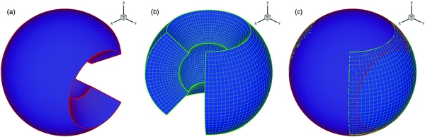
Figure 1. Yin–Yang grids. The component grid Yin (a), Yang (b), and the overlapping grid (c).
Download figure:
Standard image High-resolution imageIn Figure 1, one component grid, say, the "Yin" grid, is defined in spherical polar coordinates by

where δ = 1.5Δθ is a small buffer that minimizes the required overlap. The other component grid, the "Yang" grid, is defined by the same rule of Equation (12) but in another coordinate system that is rotated from the Yin's, and the relation between Yin coordinates and Yang coordinates is denoted in Cartesian coordinates by (xe, ye, ze) = (− xn, zn, yn), where (xn, yn, zn) are the Yin Cartesian coordinates and (xe, ye, ze) are the Yang coordinates.
An exponential relation r = ef(ξ) is used to define the radial variation of the grid, where f(ξ) is a simple function of ξ, and we set (ξ, θ, ϕ) as the coordinates of the reference space using rectangular-uniform mesh (Δξ = Δθ = Δϕ). This gives the cell sizes in the physical space as
A straightforward choice of f(ξ), i.e., f(ξ) = ξ gives Δr = rΔξ = rΔθ, which means that the cells are close to regular cubes in physical space, especially at low latitudes. Other types of f(ξ) can produce stretched or compressed mesh in the radial direction for different applications, such as fitting to active regions.
It should be noted that solving the governing equations in two different physical coordinate systems, (xn, yn, zn) for the Yin grid and (xe, ye, ze) and for the Yang grid (Kageyama & Sato 2004; Feng et al. 2011), will require solution vector transformations between two grids for data communications since expressions of a vector in the two coordinates are different. Moreover, an additional burden of the CESE method is the transformation of the solution derivatives for both the scalars and vectors (Feng et al. 2010). To avoid such cumbersome transformations, here only one physical coordinate system (x, y, z) is used with different component grids mapped to different reference spaces (ξ, θ, ϕ). Specifically, the mappings for the Yin and Yang grids are given by
and
respectively. With these mappings, all the other relations needed in Equation (11) for the establishment of a curvilinear CESE solver can be derived analytically (Jiang et al. 2010; Feng et al. 2012a).
On the boundaries where the grids overlap, solution values on one component grid are determined via interpolation from the other. We use explicit interpolation for simplicity and efficiency in parallel computation, and the grid buffer δ is suitably chosen to perform such interpolation for the overlap area (see Figure 1). In the reference space, a standard tensor-product Lagrange interpolation is used. For instance (see Figure 2 for details), the interpolation of values f at the point M(ξM, ηM, ζM) in the reference space is computed by f(M) = ∑2k = 0∑j = 02∑2i = 0f(i, j, k)PiM(ξ)PMj(η)PkM(ζ), where PMj(x) is the Lagrange interpolating polynomial  with x being ξ, η, or ζ.
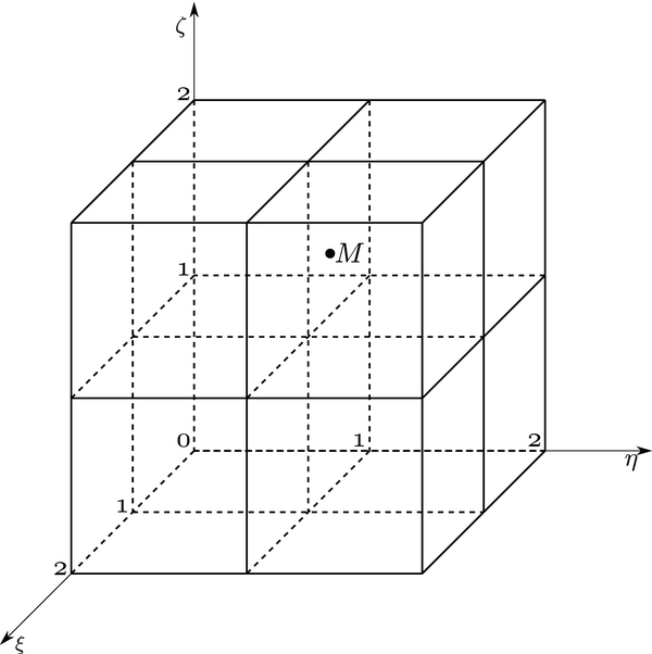
Figure 2. Interpolation of point M in the reference space: M represents a mesh point on the overlapping boundary, for example, of the Yin grid, and the 27 (33) nodes denote the Yang grid's inner mesh points that are closest to M.
Download figure:
Standard image High-resolution imageFinally, to realize the AMR on this bi-component grid and handle the data communications within PARAMESH, we divide the processors into groups with each group associated with one component grid. Each component grid is divided into self-similar blocks and distributed to the corresponding group of processors. Also the load balancing is considered carefully among these grouped processors. The interpolation of the overlapping boundaries is dealt with in a manner similar to the guard-cell filling (an operation designed in PARAMESH for communication between blocks) and arranged to be done simultaneously. A typical structure of the AMR Yin–Yang overlapping grid is given in Figure 3, which clearly shows the resolution-adaption capability of the grid system.
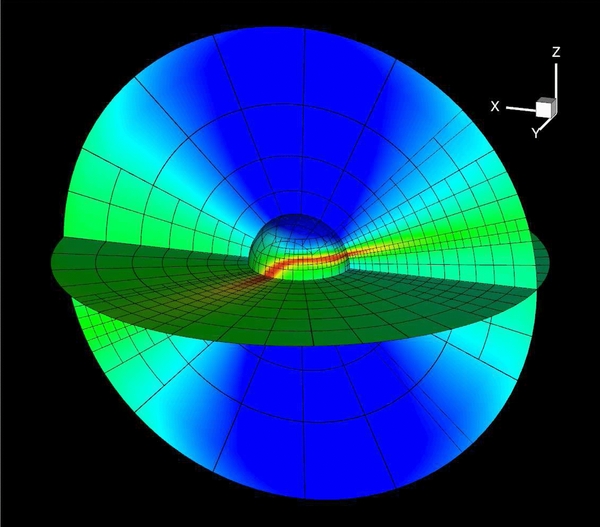
Figure 3. 3D representation of the AMR Yin–Yang grid. The inner sphere is the bottom boundary and two slices of x–z and x–y are shown. Here, the faces of computational blocks are shown without cells. The contours show the interested features captured by the adaptive resolution of the grid system: red indicates high gradient regions with high resolution and blue denotes low gradient regions with low resolution.
Download figure:
Standard image High-resolution image3. THE SURFACE FLUX TRANSPORT MODEL
The SFT model describes the radial component evolution of large-scale photospheric magnetic field with time by using the magnetic induction equation in spherical coordinates:
where the first two terms on the right-hand side of the equation describe the magnetic flux convection by differential rotation and meridional flow. Here the angular velocity of the differential rotation is given by Snodgrass (1983):

and for the meridional flow vθ, we adopt the profile given by Yeates et al. (2007):

where θmin and θmax are the poleward boundaries and C = −36 m s−1 such that the maximum flow at mid-latitudes is 16 m s−1.
The third term on the right-hand side of Equation (16) is the diffusion effect that models the random walk of magnetic flux owing to the changing super-granular convection pattern (Leighton 1964). The diffusivity is also adopted with the same value η = 450 km2 s−1 as in Yeates et al. (2007). The additional source term  can be used to describe the emergence of new magnetic flux, which is important for long-term evolution with several months or years. For short-term evolution or without new sunspots, it is often neglected.
If discretized on the θ–ϕ plane, the SFT equation can be solved numerically by the finite-difference method under the given initial-boundary value condition, i.e., the initial map of Br and a proper boundary condition. The computational domain is the entire photosphere of [0, π] × [0, 2π] and uniformly divided with grid size Δθ = Δϕ = 1°. A forward-time central-space (FTCS) scheme is used, which gives the numerical counterpart of Equation (16) as

Here i, j, and n are the indices for θ, ϕ, and t, respectively, and f denotes the numerical discretization of the right-hand of Equation (16) for short. The reason why such a simple FTCS scheme can be used is that the diffusion effect is far more sufficient for numerical stability. The time step Δt is chosen to satisfy the CFL condition:

where CFL is the Courant number and vmax is the maximum advection speed. Considering the problem of grid convergence at both poles, in the practical computation, the above finite-difference method is only used in the domain of 5° ⩽ θ ⩽ 175°. Then we can use a time step in the order of minutes and we fix it to Δt = 8 minutes while for the polar meshes, values are obtained by simply extrapolating and averaging from the solution value at θ = 5° or 175°. This is reasonable since the measured magnetic fields are least reliable at the poles. Also on the classic synoptic magnetogram that is usually provided in the format of pixels equally spaced in longitude and sine latitude, the polar region θ ⩽ 5°(⩾ 175°) is represented by almost only one pixel in the latitude direction. In the ϕ direction, boundary conditions are naturally periodic.
To initialize the SFT simulation, we produce the SEPMF based on the SOHO/MDI synchronic frames of photospheric magnetic flux, which are available online at http://soi.stanford.edu/magnetic/synoptic/. For details, refer to Hayashi et al. (2008) and X. P. Zhao et al. (2010, private communication).
For a preliminary study, we simulate the evolution from 1996 September 4 to October 29 (near the minimum of solar cycle 23) with the source term  , since no new sunspot was observed during this time interval. The numerical results given in Figure 4 clearly show the shearing and decaying of a typical bipolar active region (NOAA AR 07986 at latitude ∼ − 10°) due to surface motion and diffusion. The SFT model reproduces well the evolution of both the active region and the background field. Note that the SEPMF input for numerical computation have been smoothed to remove noise, which is done by 50 days of diffusion alone in the SFT model. Although many small-scale structures of the active region are smoothed out, the large-scale features with which we are concerned remain in the map. This simulated time-dependent map of Br is employed as boundary input to drive the coronal model. For easy manipulation of the observed data, we do not use the Yin–Yang grid in the SFT model, even though it is more compatible with the coronal grid without data interpolation. Besides the radial magnetic field variation on the bottom boundary specified by the SFT model, the other seven constraints are determined by the combination of the rotation equation of the tangential electric field on the solar surface and the projected characteristics method, which has been described in detail by Wu et al. (2006), Feng et al. (2012b), and Yang et al. (2012).
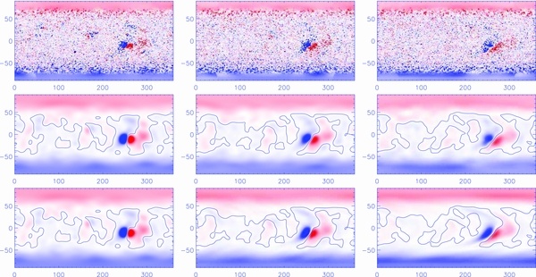
Figure 4. Comparison between the SFT-simulated SEPMFs at times on 1996 September 4, October 2, and October 29 (the three panels in the bottom row) and the observed MDI synchronic frames at the same times (the first two rows; the second row shows the smoothed version of the first row). Red and blue colors indicate positive and negative Br, respectively, with a saturation level of ±20 G. The zero contours of the observed smoothed synchronic frames and the simulated SEPMFs are also plotted for comparison of large-scale structures.
Download figure:
Standard image High-resolution image4. SIMULATION RESULTS
In this section, we present the evolution of the corona from 1996 September 4 to October 29 by coupling the SFT and coronal models.
4.1. Solution Implementation
The computational domain extends from the bottom of the corona to 35 RS and initially, the grid spacing in both θ and ϕ directions is globally 2°. Grid blocks touching the bottom surface are refined with two levels to provide the same resolution (1°) with the SFT map. An MHD equilibrium on 1996 September 4 is employed as the initial input of the data-driven simulation. The equilibrium is obtained by the same method for calculating the quasi-steady corona, i.e., the MHD relaxation of a Parker solar-wind solution and a potential magnetic field. The Parker solution is specified by the solar-surface temperature 1.8 MK and proton number density 2.0 × 108 cm−3, and the potential field is obtained using the synchronic frame on 1996 September 4, i.e., the initial map in the SFT model.
The numerical time-step constraint Δt (i.e., CFL condition) with the grid size (∼4 Mm) and Alfvén speed (∼500 km s−1) at the bottom is about several seconds. Using this time step to model months of evolution will cost tens of days with our present computational facility, which is unbearable for a preliminary study. Thus we artificially accelerate the evolution by inputting the SEPMF at a rate that is enhanced by 10 times compared to real time, as done by Lionello et al. (2005). As a result, the 8 minute cadence SEPMF provided by the SFT model is regarded as 48 s in the coronal model. We fix the time step of the bottom blocks to 4 s. Hence it takes 12 steps to achieve the cadence of the SFT maps, and data needed at the in-between steps are provided by time-linear interpolation of two successive maps. We note that this artificially enhanced variation of the maps gives us credible results since the photospheric fields changed insignificantly in this chosen period. It should also be noted that, in this section, we refer to Carrington longitude simply as longitude for simplicity.
4.2. Large-scale Coronal Structures
Figure 5 compares the simulated results with observed coronal composite images from solar surface to 6 RS. Panels (a)–(c) show the composite images observed on 1996 September 4, October 2, and October 29 from 1.15 to 2.30 Rs by the HAO/MLSO Mark-IV coronameter and from 2.30 to 6.00 Rs by the SOHO/LASCO-C2 coronagraph. The disk images were observed on the same dates by SOHO/EIT at He ii 304 Å.
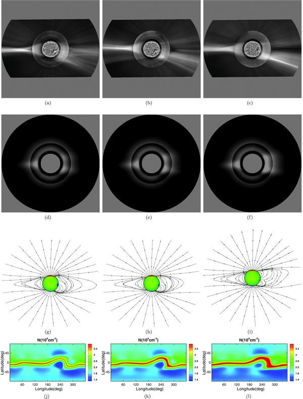
Figure 5. Comparisons of the observed and simulated coronal structures. Panels (a)–(c) give the coronal composite images on September 4, October 2, and October 29. (d)–(f) The simulated pB images for the same dates. (g)–(i) The projections of the magnetic field lines of the same dates. (j)–(l) The pseudo-color global synchronic snapshots of number density N (unit: 106 cm−3) at 2.5 RS with black lines denoting the magnetic neutral lines. In this figure, the observer on the Earth is located roughly at 180° longitude.
Download figure:
Standard image High-resolution imageFigures 5(d)–(f) are the derived white-light polarized-brightness (pB) images from the simulation for the observation dates. These images are also displayed from 1.15 to 6 RS and enhanced inside and outside 2.3 RS separately. The third row of Figure 5 gives the magnetic field lines projected on the sky planes with the color contours of surface Br, and the three panels in the bottom row show the total calculated surface distribution of number density N at 2.5 Rs on 1996 September 4, October 2, and October 29.
In the simulated period, the structure of the coronal streamers changed very little, as shown in Figure 4. The equatorial "jet" that dominates the east limbs of Figures 5(a)–(f) is a typical helmet streamer at solar minimum, showing a simple quasi-dipole magnetic topology. In the west limbs, the presence of multiple bright structures is due to the warp of the magnetic field neutral line around the longitude of ϕ = 270° (see the neutral line plot in the last row). From a detailed examination one can see the gradual separating of the west limb streamers, and these features are well represented by the evolution of the magnetic field lines. Figures 5(j)–(l) also show that the number density in the streamers grows slightly, which is consistent with the pB images.
Figure 6 compares the simulated coronal holes with those from the SOHO/EIT 195 Å observations. The three panels in the top row are the EIT 195 Å Carrington synoptic maps of Carrington rotations 1913, 1914, and 1915. The dark vertical strips in this figure denote the observation gaps. On these maps, the dark regions are typically identified as the coronal holes with lower levels of emission due to lower plasma densities and temperatures. The coronal holes are believed to be associated with regions of an open magnetic field stretched by the solar wind. By tracing the 3D field lines in the numerical results, we produce maps to identify open-field (black) and closed-field regions (white) on the Sun (the second row of the figure). In CR 1913 the most conspicuous observed feature is the elephant-trunk-like northern extending coronal hole (ECH) at approximately 270° longitude, which is also captured by the MHD model. The simulation results show that the longitudinal width of the ECH at 40° latitude decreases from 25° in CR 1913 to 15° in CR 1915. Meanwhile, the longitudinal width of the ECH at the solar equator increases by 10°. It should be noted that the southern ECH also reaches the equator approximately at 240° longitude with a long channel, and it becomes increasingly inclined over time because of the differential rotation included in the SFT model. All these features of the CHs and their evolutions are clearly shown by both the EIT images and the simulated maps. In addition, a visible shrinking of the polar coronal holes during the simulated period from CR 1913 to CR 1915 can be seen in the modeled maps. This is probably due to the combined effect of poleward meridional flows and the diffusive process in the SFT model. The observed images also show such an evolutionary trend, even though it is not as pronounced as the simulation shows.
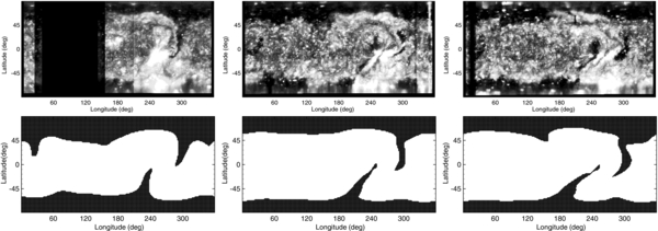
Figure 6. Comparisons of the coronal-hole locations: SOHO/EIT 195 Å synoptic images (the first row) and simulated coronal-hole maps on 1996 September 4 (CR 1913), October 2 (CR 1914), and October 29 (CR 1915). In the second row, dark regions denote the coronal holes.
Download figure:
Standard image High-resolution image4.3. Magnetic Field in the Active Region
Figure 7 shows the magnetic evolution of AR 07896 by plotting the 3D field lines (black lines) over the contours of the radial field (pseudo-color image). The first row gives the MHD results, and the second row the potential field extrapolations of the corresponding SEPMF. From left to right, the time sequence is the same as that of Figure 5.
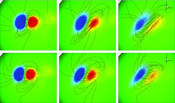
Figure 7. Simulated magnetic evolution of the active region (the first row) and comparison with the potential field extrapolations. From left to right, the images correspond to the results on 1996 September 4, October 2, and October 29. Black lines with arrows denote the magnetic field lines and their directions. The background image stands for the contours of the radial field. Red indicates positive Br and blue indicates negative Br, with a saturation level of ±20 G.
Download figure:
Standard image High-resolution imageAt first glance, one clearly recognizes that the field is getting weaker and the shear is growing stronger, which results from the surface diffusion and the surface flow of the differential rotation and meridional motion. In order to demonstrate the coronal responses to these photospheric physical processes, we show the 3D magnetic field topologies of the same time sequence in Figure 8 with the central meridian of 180° longitude. From this figure, we can find that the closed field lines originating from the edges of the active region extend outward almost to about 10 Rs, the outer boundary of Figure 8, which probably results from the large gradient of the magnetic force due to the strong magnetic field associated with the active region, the artificial heating added in the MHD model, and the enhanced differential rotation (Mackay & van Ballegooijen 2006) included in the SFT model. In Figure 9, we present 3D views of the simulated field lines on the same dates as those in Figure 8, but the longitude of the central meridian is 220°. From this figure, we find that the closed magnetic field lines in the coronal streamers only extend outward to 5–7 Rs. We also note that the closed-field region lies within 5 Rs in Linker et al. (2011), who explored coronal evolution by introducing an artificial surface flow in a small region of the solar surface. The artificial surface flow introduced by Linker et al. (2011) was far below the enhanced differential rotation used in the present paper. Therefore, the strong magnetic field in AR 07896 and the enhanced differential rotation should be two important reasons for the large radial extent of the closed-field regions displayed in Figure 8. In addition, this phenomenon was also investigated in detail by Lionello et al. (2005), who analyzed coronal response to enhanced photospheric differential rotation with the help of the resistive MHD model. Small loop structures near the Sun may be formed through the processes of magnetic reconnection discussed in Lionello et al. (2005) due to unavoidable numerical viscosity and the release of plasmoids during magnetic reconnection that will probably become the near-Sun counterparts of the small-scale transient events observed in interplanetary space (e.g., Kilpua et al. 2009; Foullon et al. 2011). Meanwhile, magnetic reconnection is also required in order to understand the rigid rotation of the coronal holes (Wang et al. 1996; Zhao et al. 1999). However, in-depth analysis is beyond the scope of this paper and will be investigated in our future studies.

Figure 8. 3D views of the field lines in the numerical simulation of the same time sequence in Figure 7 (left to right) with the central meridian located at 180° longitude. Note that this figure is plotted in a view different from Figure 7 to show more clearly the 3D field lines associated with the AR. The field lines in these panels are rendered with different colors and traced from the same footpoints at the coronal base.
Download figure:
Standard image High-resolution image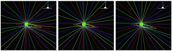
Figure 9. 3D views of the field lines in the numerical simulation on the same dates as those in Figure 8, but the longitude of the central meridian is 220°.
Download figure:
Standard image High-resolution imageSecond, the field lines gradually become aligned to the polarity neutral line (PNL) due to shearing, especially on 1996 October 29 (CR 1915); some field lines are almost parallel to the PNL, which shows the growth of nonpotential energy. This field configuration is also supported by observations. Figure 10 shows the Hα images of the solar disk from Big Bear Solar Observatory (BBSO) and the MDI full-disk magnetogram on 1996 October 23, when the active region is roughly at the central meridian. Note that above the active region a large-scale filament lies along the PNL. To support the filament, the field lines are commonly believed to be approximately along the long axis of the filament (Low 1996), although the fine-structure field could be complicated by multi-twisted ropes (Lionello et al. 2002). Such continuous evolution of nonpotential magnetic field configuration as well as the coronal plasma flows can hardly be reproduced by a static model such as the potential field source surface model or nonlinear force-free models (e.g., Riley et al. 2006; Riley 2007; Wiegelmann 2008), which neglect inertial effects and gas pressure and incorporate no temporal history of the fields.
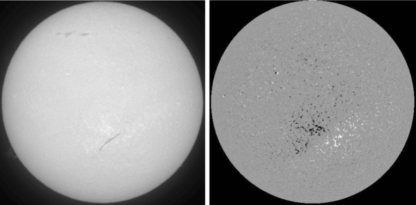
Figure 10. Hα image from BBSO (left) and the MDI full-disk magnetogram (right) on 1996 October 23.
Download figure:
Standard image High-resolution image4.4. Solar Wind at 0.1 AU
In this section, we show the evolution of the solar-wind parameters, e.g., the number density N, the radial velocity vr, and the magnetic flux Br at roughly 0.1 AU (21.5 RS) in Figure 11. These near-Sun solar-wind parameters are important and can serve as boundary conditions for a heliospheric model that is focused on the outer corona and interplanetary space (e.g., Odstrcil et al. 2004a, 2004b; Detman et al. 2006; Taktakishvili et al. 2011). Figure 11 reveals that the neutral line warps around ϕ = 250° with slightly enhanced density, although the variation is small. The velocity evolution shows that the model successfully produces bimodal solar-wind structure with a high speed of ∼600 km s−1 and a low speed of ∼300 km s−1, which is consistent with previous simulations of the empirical model for solar minimum (McGregor et al. 2011). Furthermore, we compare the numerical velocity distribution with those derived by the empirical WSA model (McGregor et al. 2011),

where Ca is defined in Equation (9). Figure 12 presents the results based on the synoptic maps of the observed magnetic field. Basically, the overall structures of the velocity obtained from the MHD simulation in Figure 11 and the WSA model in Figure 12 are roughly consistent. Differences between them are mainly twofold: the MHD results present a slightly lower value (by ∼50 km s−1) of the velocity of the fast solar-wind flow than the empirical WSA model and at the same time gives a much narrower coronal streamer.
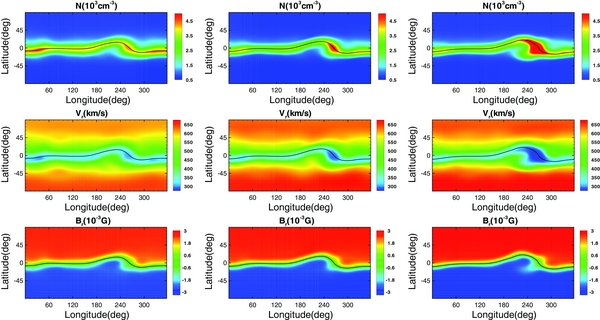
Figure 11. Entire surface distribution of the solar-wind parameters simulated at 0.1 AU on 1996 September 4, October 2, and October 29 from left to right. The first row gives the number density N, the second row the radial velocity vr, and the last row the magnetic flux Br.
Download figure:
Standard image High-resolution image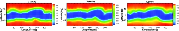
Figure 12. Solar wind velocity at 0.1 AU, computed by the empirical WSA formula (21) of fs and θb based on the Carrington synoptic maps of the observed photospheric magnetic flux in CRs 1913, 1914, and 1915 centered at 1996 September 4, October 2, and October 29, respectively.
Download figure:
Standard image High-resolution image
5. CONCLUSIONS
By combining the SFT model and an MHD coronal model, we developed a dynamic model for the evolution of the global corona driven by the time-varying photospheric magnetic field. The main features of this data-driven model are as follows.
- 1.We employ the SFT model to produce the self-consistent and time-varying SEPMF with the observed synoptic maps, which are used to drive the MHD model.
- 2.The use of two logically Cartesian reference spaces, transformed from the overlapping Yin–Yang grid, can avoid singularities and grid convergence at both poles, and simultaneously simplify the implementation of AMR.
- 3.Coupling of the SFT model and the 3D coronal model occurs via the rotation equation of the tangential electric field and the projected characteristic method. This method can couple the bottom input data, the SFT model, and the global coronal model in a more compatible and reliable way, particularly considering the deficiency of observed information.
A preliminary application of the data-driven model is validated by simulating the coronal evolution from 1996 September 4 (CR 1913) to October 29 (CR 1915). In the simulated interval, the main variation shown in the observed synoptic maps or the SFT simulated SEPMFs is the decay of a bipolar active region in the background of a slowly evolving quasi-dipole field. By comparison with the SOHO/EIT, MLSO, and LASCO images, we show that the model is able to generate the general structures of the global corona, such as coronal streamers, the locations of coronal holes, and their evolutions. Also the nonpotential magnetic configuration overlaying the active region, which is supported by the observation of a quiescent filament in the Hα image, is partially reproduced by the model. However, the radial extent of the closed-field regions associated with the active region which is too large is present in our simulation likely due to the large gradient of magnetic force, the artificial heating added in the MHD model, and the enhanced differential rotation included in the SFT model.
For future wider applications, the emergence of new magnetic flux (i.e., the source term) should be incorporated into the SFT model to maintain observational accuracy over long periods of time, and the insertion of the new flux into the maps should also be done in a self-consistent way to drive the 3D physics-based MHD model. In the present simulation, the ideal MHD is used without the resistive term, because the magnetic topology of the field changes little during evolution. An intrinsic resistivity of the numerical scheme, although small, is sufficient to account for the small change in magnetic topology. A more complex or general field configuration, such as the continuous inserting of newly emerging flux, may require a significant change in topology, which is a basic mechanism for the replacement of old magnetic flux with new flux. To deal with such problems, we require a more physics-based model. Since this paper is devoted to the construction of a basic framework for the data-driven model with a bias on numerical techniques (e.g., the grid systems, the numerical scheme, the computational technique, and the boundary conditions), modeling with more physical considerations will be left to future work.
In the present paper, we have performed a global solar coronal simulation by smoothing out the small-scale information in the active region. However, most of the solar eruptions are closely related to those small-scale fields by the basic processes hidden there, including the building-up of magnetic energy and triggering of instability. Simulations with a local coronal model that is focused on a single active region can possibly provide the details of these processes, but failed to provide the overall picture of the eruptions in the corona. Moreover, the active regions cannot be isolated since they generally interact with overlaying large-scale fields. With the parallel-AMR computational technique and more available observed data, e.g., the full-disk and high-cadence vector magnetograms such as the observation with SDO (Henney et al. 2009; Scherrer et al. 2012; Liu et al. 2012), we hope that our new data-driven model can simultaneously address the small-scale fields of active regions (Jiang et al. 2011) and the global corona and/or interplanetary space (Feng et al. 2012a, 2012b) to possibly provide a numerical tool for the study of the initiation and evolution of solar explosive phenomena and their interplanetary evolution process.
This work is jointly supported by the National Basic Research Program (973 program) under grant 2012CB825601, the Chinese Academy of Sciences (KZZD-EW-01-4), the National Natural Science Foundation of China (41031066, 40921063, 40890162, 41074121, and 41074122), and the Specialized Research Fund for State Key Laboratories. Dr. S. T. Wu is supported by AFOSR (grant FA9550-07-1-0468), AURA Sub-Award C10569A of NSO's Cooperative Agreement AST 0132798, and NSF (grant ATM-0754378). The numerical calculation has been completed on our SIGMA Cluster computing system. The PARAMESH software used in this work was developed at NASA Goddard Space Flight Center and Drexel University under NASA's HPCC and ESTO/CT projects and under grant NNG04GP79G from the NASA/AISR project. The Big Bear Solar Observatory/New Jersey Institute of Technology is acknowledged for the Hα image. SOHO is a project of international cooperation between ESA and NASA. The authors express their heartfelt thanks to the anonymous reviewer for constructive suggestions.