

Abstract
The Comité international des poids et mesures (CIPM) has projected a major revision of the International System of Units (SI) in which all of the base units will be defined by fixing the values of fundamental constants of nature. In preparation for this we have carried out a new, low-uncertainty determination of the Boltzmann constant, kB, in terms of which the SI unit of temperature, the kelvin, can be re-defined. We have evaluated kB from exceptionally accurate measurements of the speed of sound in argon gas which can be related directly to the mean molecular kinetic energy,
 . Our new estimate is kB = 1.380 651 56 (98) × 10−23 J K−1 with a relative standard uncertainty uR = 0.71 × 10⁻⁶.
Export citation and abstract BibTeX RIS
1. Introduction
1.1. Introduction
1.1.1. Background.
The current definition of the kelvin [1, 2] (the fraction 1/273.16 of the temperature of the triple-point of water) has proved adequate for more than 50 years. However, the nature of temperature as an intensive quantity leads to difficulties in 'scaling' the unit to higher and lower temperatures. In this sense the definition itself limits the accuracy achievable at temperatures that differ significantly from the temperature of the triple-point of water (TTPW).
The CIPM now proposes [3] to introduce a new definition of the kelvin, which will simply state that the kelvin has a value consistent with a defined value of the Boltzmann constant, kB. This links the value of the unit of temperature, the kelvin, to the value of the unit of energy, the joule (1 J = 1 kg m2 s−2) and is independent of any particular temperature. In this conception, the Boltzmann constant would be fixed with no associated measurement uncertainty. In order to make the transition from one unit definition to another as seamless as possible it is desirable to have a low-uncertainty estimate of the value of kB in the current unit definition.
1.1.2. Overview of the acoustic resonance technique.
Many techniques can be used to estimate kB, but a recent review [4] concluded that acoustic techniques were likely to achieve the lowest uncertainty. One reason for this is the strikingly simple relationship between the limiting low-pressure speed of sound c0 in a monatomic gas and the root-mean-squared speed of the molecules, vRMS:
 . In terms of macroscopically measurable parameters this becomes
 where γ0 is the ratio of the principal heat capacities of the gas in the limit of low pressure, T is the thermodynamic temperature and M is the molar mass of the gas. The molar gas constant R is defined by R = NAkB where NA is the Avogadro constant. Rearranging for kB we find

Since γ0 = 5/3 exactly for monatomic gases, and NA is known with a relative standard uncertainty uR = 0.044 × 10⁻⁶ [5] experimentally, the challenge is to measure M, T and
 with low uncertainty. Importantly, and in contrast with PVT gas thermometry techniques, the speed of sound is only weakly dependent upon pressure. There is thus no need to determine the pressure with the same or lower fractional uncertainty than is required for our estimate of kB.
Low uncertainty in M requires meticulous gas-handling, and quantification of isotopic variations and chemical impurities, which can also affect γ. Low uncertainty in T is achieved by carrying out the experiment close to the temperature of the triple-point of water, TTPW. The entire experiment can be viewed as a primary measurement of the product kBTTPW, but because TTPW is currently defined to be 273.16 K exactly, measuring the product allows an estimate of kB.
Low uncertainty in
is achieved by measurements in a combined acoustic and microwave resonator (figure 1). The microwave resonances allow estimates of the dimensions of the resonator as a function of temperature and pressure, which may then be combined with measurements of the frequencies of acoustic resonances to yield an experimental estimate for the speed of sound, cExp.

Figure 1. Conceptual illustration of the operation of a combined acoustic and microwave resonator. Microwaves: the radius of the resonator is estimated from microwave measurements of up to eight TM1n resonance triplets. The frequencies must be corrected for the dielectric properties of argon gas. The uncertainty associated with this correction becomes smaller at low pressure. The radius at zero pressure is used in the estimate of the limiting low-pressure speed of sound. Acoustics: The speed of sound is deduced from the frequencies of several radial acoustic resonances and kB is deduced from the zero-pressure limit. In order to obtain this, several pressure-dependent frequency corrections must be applied.
Download figure:
Standard image High-resolution imageWe then deduce the limiting low-pressure speed of sound c0 by extrapolating
 to the limit of P = 0. However, before this is done, both microwave and acoustic resonant frequencies must be corrected for pressure-dependent effects. The acoustic corrections arise mainly at low pressure from the thermal boundary layer (TBL) between the gas and the resonator wall. The microwave corrections are proportional to pressure and arise from the change in the speed of light due to the polarizability of argon.
We examine only the (0, n) acoustic resonances which have a purely radial variation in sound pressure level. We choose these modes because they do not suffer from viscous losses at the boundary with the resonator wall, and thus they have a higher Q-factor than most acoustic modes. Additionally they have a particularly simple interaction with the mechanical vibrational modes of the resonator shell [6] and are relatively unaffected by smooth deviations from sphericity. In our analysis we seek a single value of
to describe all the acoustic data from six resonances, each of which has several corrections which must be made without any adjustable parameters. The extent to which the data are truly self-consistent from mode to mode provides a strong check on several underlying assumptions, making it possible to detect a range of potential systematic errors.
A perfectly spherical resonator is acoustically simple, but unsuitable for simultaneous use as a microwave resonator because no singlet microwave resonances exist. The lowest degeneracy of microwave modes is three, and even tiny manufacturing imperfections and the joint between the two hemispheres will partially split these triplet resonances, distorting the line-shape and introducing uncertainty into the estimation of the mean frequency. It is the mean frequency of the triplet microwave resonances which is related to the radius [7]. The radius estimated by the microwave technique is known as the equivalent radius aeq, defined as the radius of a perfect sphere with the same volume as the experimental quasisphere,
![$a_{{\rm eq}}= \sqrt[3]{3V/4\pi}$](https://content.cld.iop.org/journals/0026-1394/50/4/354/revision1/metro471348ieqn006.gif) .
.
Introducing a triaxial shape modification allows the triplet components to be individually resolved [7] and improves the precision with which the mean frequency, and hence the resonator dimensions, may be determined. Because of the high electrical conductivity of copper the microwave resonances are narrow, allowing the triplet components to be individually resolved with only a small deviation from sphericity (±0.05%). This shape perturbation produces a small, but calculable shift of the acoustic resonances [8–10].
1.2. Experimental details
1.2.1. Measurements.
Our estimate of kB is deduced from three sets of isothermal measurements of cExp(P) carried out close to TTPW. We refer to these as Isotherms 3, 4 and 5. Isotherms 1 and 2 were used for establishing the operation of the cryostat and resonator, and Isotherms 6 and beyond are being used to estimate differences between the thermodynamic temperature and the temperature estimated according to the International Temperature Scale of 1990, T90.
1.2.2. Resonator.
Our speed of sound measurements were carried out inside the NPL–Cranfield resonator NPLC-2 [11] (figure 2). This is constructed from two copper hemispheres whose internal surfaces were cut so that, when assembled, they create a triaxially ellipsoidal inner surface defined by

with a = 62.0 mm, ε1 = 0.0005 and ε2 = 0.001. This produces a resonator with volume of approximately 1 L which we considered large enough to make surface perturbations relatively small while minimizing temperature gradients that might occur across a larger resonator.
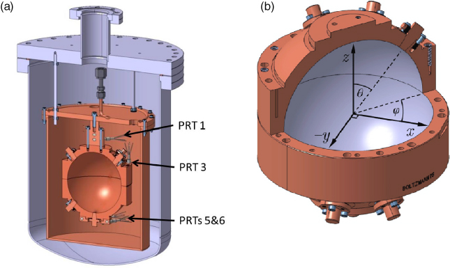
Figure 2. (a) Cross-section through the apparatus showing the NPL–Cranfield resonator NPLC-2 suspended within an isothermal enclosure within an outer 25 L pressure vessel. The pressure vessel was immersed in a stirred liquid bath at a temperature of approximately −0.2 °C. Also visible are some of the PRTs positioned in the neck, the equator and the south pole. In use, the argon gas flows into the resonator at a rate of 7.4 × 10⁻⁷ mol s−1 (1 sccm) and then passes into the surrounding isothermal volume where the pressure is measured. The internal pressure is close to the external pressure, with the small difference being determined from microwave measurements of the dielectric constant of the argon gas. (b) Cut-away view of the resonator sphere showing the showing the coordinate system. Notice the –y-axis is shown. The outer cylindrical surface was cut at the same time as the inner surface so that when the hemispheres are assembled, good alignment between the two outer cylindrical surfaces ensures good alignment of the inner surfaces.
Download figure:
Standard image High-resolution imageEach hemisphere has four blank plugs, which initially protruded beyond the inner surface, but during manufacture these were machined back to make a nearly perfect match with the surrounding quasispherical surface. Probing using a coordinate measuring machine showed that the entire surface of each quasihemisphere was within 1.5 µm of its design form [11]. Our low uncertainty of measurement is largely due to the near-perfect shape and surface condition achieved by fabrication using ultra-precision diamond-turning techniques [12]. After machining, the plugs were removed and modified (figure 3, table 1) to accept microwave antennas, acoustic transducers and gas inlet and outlet tubes.
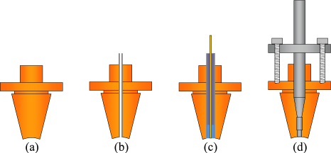
Figure 3. Designs of the four types of plugs. (a) A blank plug. (b) Gas inlet and outlet ducts. (c) Microwave antenna with the central conductor adjusted to be flush with the spherical surface, and the surrounding volume filled with epoxy resin. (d) Acoustic transducer, in this case the microphone, including the pre-amplifier.
Download figure:
Standard image High-resolution imageTable 1. Summary of plugs in NPLC-2. Angles θ and φ refer to the equivalent angles in figure 2.
| Plug | Function | θ | φ | Notes |
|---|---|---|---|---|
| Northern hemisphere | ||||
| 1 | Microwave in | 45° | 45° | In between x-, −y and z-axes |
| 2 | Gas out | 45° | −45° | |
| 3 | Gas in | 45° | 135° | |
| 4 | Blank | 45° | 90° | |
| Southern hemisphere | ||||
| 5 | Acoustics in | 180° | 0 | 'South pole' |
| 6 | Acoustics out | 140.8° | 45° | Position chosen to minimize interference between the (0,2) and (3,1) resonances |
| 7 | Blank | 135° | −90° | |
| 8 | Microwave out | 135° | −45° | In between x, −y and −z axes |
In operation the resonator was suspended from the lid of a copper container designed to create a nearly isothermal environment. The copper container—which had holes to allow gas to enter and leave—was suspended inside a stainless-steel pressure vessel, and the pressure vessel was immersed in a temperature-controlled bath at approximately –0.2 °C.
1.2.3. Acoustics.
Plugs 5 and 6 were removed and replaced with plugs modified to accept Gras type 40DP acoustic transducers with a diameter of 3.2 mm. The inner faces of the plugs were carefully ground to match the curvature of the plugs they replaced as closely as possible. Microwave measurements were made before and after the replacement to assess the perturbation to the inner surface of the resonator (section 2.3.1).
One transducer was used as a sound source by using a transmitter adapter (Gras RA0086). It was polarized to 130 V and driven by a Krohn-Hite 7602 M amplifier with a sinusoidal waveform from an SRS DS345 oscillator with its time-base linked to a 10 MHz rubidium clock (SRS SIM 940). The clock was periodically checked against a 10 MHz signal derived from NPL's primary frequency standard and never found to differ by more than one part in 1011. The same clock was also used to drive the time-base on the Agilent N5230A PNA-L Network Analyser used for microwave measurements.
By linking the other transducer directly to an amplifier (Gras 26AC) we reduced stray capacitance and improved signal-to-noise performance. However, despite lowering the supply voltage, the amplifier dissipated ∼1.7 mW continuously—a significant amount of heat to dissipate close to the resonator. The effect of the power dissipation is discussed in section 2.2.
1.2.4. Gas inlet and outlet.
The inlet duct fitted into plug 3 was constructed out of 0.634 mm diameter tube 124 mm long connected to a 0.900 mm diameter tube 4 m long. This was thermally attached to the copper lid of the isothermal shield in order to temperature-condition the incoming gas. The outlet duct fitted into plug 2 was constructed out of 0.522 mm diameter pipe 62 mm long and led directly to the isothermal enclosure which was at the same pressure as the enclosing pressure vessel. At 100 kPa and a flow rate of 7.4 × 10⁻⁷ mol s−1 (1 standard cubic centimetre per minute (sccm)) the flow speed of gas entering the resonator was approximately 50 mm s−1 and the nominal residence time in the resonator was approximately 17 h. In the same conditions the flow speed of gas in the outlet duct was approximately 78 mm s−1, which we calculated was sufficient to prevent significant back-diffusion of impurities from the outer pressure chamber.
1.2.5. Pressure and flow measurement and control.
The pressure of the gas within the resonator was controlled by measuring the pressure in the vessel containing the resonator with a GE Druck DPI 150 pressure indicator. The measured pressure was compared with a set pressure and the results fed back to a mass-flow controller (MFC1) at the inlet of the gas-handling system. Typically pressure fluctuations had a standard deviation of 0.6 Pa at all pressures. Before the measurements described in this work, we detected that the DPI 150 calibration was drifting by several tens of pascal each day. For subsequent isotherms we used a Ruska 7000 as an additional pressure indicator, and zeroed the device before and after each data acquisition run. The Ruska 7000 was calibrated at NPL before and after this work and the table of corrections was unchanged within the measurement uncertainty of approximately 30 parts in 106, i.e. 3 Pa at 100 kPa.
The flow rate through the resonator was set by a second mass-flow controller (MFC2) at the outlet of the pressure chamber. The combination of the two MFCs allowed stable pressures and flows to be established. In order to ensure good flow control at low flow rates, while allowing the pressure to be changed quickly, MFC1 and MFC2 were each parallel combinations of two MFCs: a low flow (0–10 sccm) and a high flow (0–500 sccm) device. We used a flow rate of 1 sccm for all measurements, and the effect of this flow on the resonant frequencies is discussed in section 2.4.2.
The pressure within the resonator was inferred by accounting for the differences in height and temperature between the Ruska 7000 and the centre of the resonator, and then additionally for the pressure drop as gas flowed through the outlet duct. The impedance of the outlet was measured by holding the pressure in the outer vessel constant, and measuring the change in the dielectric constant of the gas within the resonator as the flow was varied. The inferred pressure within the resonator was checked by dielectric constant measurements (section 2.3.2) and found to be consistent with the Ruska 7000 within approximately 10 Pa at all pressures.
1.2.6. Temperature control.
Temperature control was achieved using feedback from one of two type 5187L Tinsley capsule standard platinum resistance thermometers (cSPRT) installed on the neck supporting the resonator. The cSPRT was read by a Tinsley Senator bridge and the bridge output was used as the feedback signal for a PTC10 temperature-controller. The resonator was heated indirectly by a silicone heater pad attached to the outside of the isothermal enclosure. The remaining cSPRT on the neck and the four cSPRTs on the equator and the south pole were read by an ASL F18 bridge and used to deduce the resonator temperature. The results are described in section 2.2 along with an evaluation of measurement uncertainty.
1.2.7. Data acquisition.
At each pressure we measured the (0, 2) to (0, 9) resonances and extracted estimates of the resonant frequency f(0,n) and half-width g(0,n), taking 40 data points in the range ±3g(0,n), around the peak of each resonance, first with increasing frequency and then with decreasing frequency. The rising and falling data for each frequency were averaged and fitted to a complex Lorenztian function with a linear background:

where the vector symbol indicates that a quantity has both in-phase and out-of phase components. From this analysis f(0,n) and g(0,n) can be deduced.
Additionally each data set was also fitted by a similar function with an additional quadratic term and a comparison made between the fitted results and their associated uncertainties. The linear background fit had the lowest uncertainties for all modes at all pressures with the exception of the (0, 7) and (0, 9) resonances at lower pressures. These modes are affected by broadening of neighbouring non-radial modes, and so for the (0, 7) and (0, 9) modes, the quadratic background fit was used at low pressure.
1.2.8. Corrections to f(0,n).
The experimentally determined acoustic resonant frequencies f(0,n) require several corrections Δf(0,n) before they can be used to make an experimental estimate of the speed of sound, cExp, using

where ξ(0,n) is the appropriate eigenvalue [8, 9], and aeq is the so-called equivalent radius discussed in section 1.2.9.
The corrections Δf(0,n) take account of the perturbing effect of: the ducts bringing gas into and out of the resonator, the acoustic transducers, bulk dissipation in the gas, the effect of the shape deformation, and differences in temperature away from TTPW. These corrections differ from mode to mode, but are small, typically a few parts in 106, and have been extensively discussed in the literature [7, 11, 13–16].
However the correction arising from the TBL between the gas and the walls of the resonator is large. It increases as the pressure falls as
 and for our resonator at one atmosphere amounts to approximately 214 parts in 106 for the (0, 2) resonance (figure 4(a)).
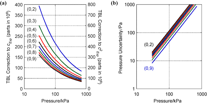
Figure 4. (a) Magnitude of the TBL correction to cExp(P) (left-hand axis) and
(right-hand axis) for the (0, 2) to (0, 9) resonances for a spherical resonator of volume 1 L. Note that the pressure axis is logarithmic. (b) The uncertainty in the pressure measurement (in pascal) required for 0.1 parts in 106 concomitant uncertainty in
. The uncertainty in
arising from the estimation of the TBL is discussed in section 2.4.4. Note that both axes are logarithmic.
Download figure:
Standard image High-resolution imageSince kB is inferred from
 it is doubly sensitive to this correction and in order to evaluate it correctly it is important to measure the pressure with low uncertainty. Figure 4(b) shows the pressure uncertainty required to correct the frequencies of the (0, 2) to (0, 9) resonances with a relative standard uncertainty of uR = 0.05 × 10⁻⁶, which at low pressure would add an additional relative standard uncertainty of uR = 0.1 × 10⁻⁶ on estimates of
used to estimate kB. Pressure errors on the order of 100 Pa such as have been reported in the literature [14, 15] can lead to distortion of
and cause significant errors in the inference of
.
it is doubly sensitive to this correction and in order to evaluate it correctly it is important to measure the pressure with low uncertainty. Figure 4(b) shows the pressure uncertainty required to correct the frequencies of the (0, 2) to (0, 9) resonances with a relative standard uncertainty of uR = 0.05 × 10⁻⁶, which at low pressure would add an additional relative standard uncertainty of uR = 0.1 × 10⁻⁶ on estimates of
used to estimate kB. Pressure errors on the order of 100 Pa such as have been reported in the literature [14, 15] can lead to distortion of
and cause significant errors in the inference of
.
1.2.9. Equivalent radius.
In order to convert measurements of the frequencies of acoustic resonances into estimates of the speed of sound, the 'equivalent' radius aeq of the resonator must be determined (equation (4)). The equivalent radius corresponds to the radius of the perfect sphere with the same volume as our experimental 'quasisphere'
![$(a_{{\rm eq}}=\sqrt[3]{3V/4\pi})$](https://content.cld.iop.org/journals/0026-1394/50/4/354/revision1/metro471348ieqn009.gif) and differs by only a few nanometres from the average radius. In this experiment aeq is deduced from a set of microwave resonances acquired at the same time as the acoustic resonances. Our estimate is the culmination of research executed over several years, both at NPL and at other laboratories world-wide, and is supported by four key results.
and differs by only a few nanometres from the average radius. In this experiment aeq is deduced from a set of microwave resonances acquired at the same time as the acoustic resonances. Our estimate is the culmination of research executed over several years, both at NPL and at other laboratories world-wide, and is supported by four key results.
The first result is the solution of the electromagnetic modes in a triaxial ellipsoid. The first-order solution was calculated by Mehl [7], who also conjectured a second-order solution [17] which was later confirmed by the numerical method of Edwards and Underwood [18]. Collectively these works provide a sound theoretical basis for the inference of aeq from microwave data such as those shown in figure 5. In this work we infer aeq from four distinct microwave resonances (section 2.3), and the level of agreement between these estimates is typically on the order of a few nanometres, less than a part in 107 of the resonator radius.

Figure 5. The TM11 microwave resonance showing the triplet structure caused by the triaxial shape. The blue circles are data points and the red curve is a fit.
Download figure:
Standard image High-resolution imageThe second result is the experimental confirmation of the microwave measurement by comparison with other techniques. In preparation for measurement of the Boltzmann constant, we checked the microwave radius measurement by comparison with other techniques. To achieve this we measured aeq for a second resonator NPLC-1 (nominally identical to NPLC-2) with a coordinate measuring machine [11], with microwave spectroscopy and using pyknometry with water [19]. The experiments revealed no evidence of any systematic deviation with comparison uncertainties of 187 nm (3 parts in 106) and 37 nm (0.6 parts in 106), respectively. This agreement is remarkable because the pyknometry estimate is traceable to SI base units through mass and density standards rather than time and dimensional standards. The pyknometric determination required coating NPLC-1 with benzotriazole [20] to prevent corrosion by the water, a step which introduced additional uncertainties and so this was not undertaken for NPLC-2. These intercomparisons support our understanding that the microwave technique is not subject to any unidentified systematic biases other than those identified from the internal consistency of the microwave data themselves.
The third is the estimation of the perturbation to the measured microwave resonance frequencies when the surface of the triaxial ellipsoid is altered, for example by the insertion of acoustic transducers and microwave probes. In section 2.3.1 we describe the effect of introducing acoustic transducers into the resonator and of modifying the microwave antennas, and show that these are in agreement with expectations.
The final result is an evaluation of the dielectric corrections caused by the presence of argon. An assessment of these corrections provides an important check on our estimate of the gas pressure within the acoustic resonator [21] (section 2.3.2).
We limited our microwave analysis to the TM1n triply-degenerate microwave resonances, because we were able to calculate the antenna perturbations from first principles using a combination of electromagnetic analysis and finite-element modelling [22]. The disadvantage of this choice is that TM modes are more strongly perturbed by possible dielectric layers on the surface of the resonator. Nonetheless, the compromise yielded acceptable results.
1.2.10. Choice of gas.
In principle any pure gas could be used, but for the lowest uncertainty a monatomic gas is necessary, and if the gas is to be flowed through the resonator, the cost of the gas limits the choice to either argon or helium. The advantages of using helium are that it is nearly mono-isotopic, and its thermal conductivity—on which estimates of the TBL depend—can be more accurately calculated [23].
Nonetheless we chose to use argon because its density is more similar to that of air in which acoustic transducers have been designed to operate. This significantly improves the signal-to-noise ratio at a given pressure. Additionally the TBL correction is smaller, the effect of common impurities is less, and the gas is compatible with the quartz Bourdon gauge in our Ruska Model 7000 pressure indicator that we used for traceable pressure measurements.
1.2.11. Previous work.
Our approach builds on techniques developed in our previous work [15, 16] and the two previous lowest uncertainty estimates of kB. The seminal 1988 work by Moldover et al [13] (uR(kB) = 1.8 × 10⁻⁶) used a 3 L stainless-steel spherical resonator and employed two sophisticated techniques for reducing the uncertainty in estimates of M and aeq. They determined M by measuring the difference in speed of sound between their working gas and a sample of nearly mono-isotopic 40Ar. To determine aeq they carried out an audacious pyknometry experiment that involved cooling the resonator to TTPW, filling it with mercury of uniquely characterized density, and then measuring the mass of mercury that just filled the resonator. The LNE 2011 work by Pitre et al [14] (uR(kB) = 1.24 × 10⁻⁶) used a 0.5 L copper quasi-spherical resonator. They determined M by a gravimetrically traceable isotope-ratio mass spectrometry measurement [24] and estimated aeq using simultaneous microwave resonance spectrometry [7, 25].
2. Results
2.1. Molar mass
2.1.1. Introduction.
Our estimate of the molar mass of the argon gas used in this work is based on measurements of its isotopic and chemical composition. We discuss first the isotopic analysis which dominates our uncertainty and then in turn the effect of chemical impurities considered in three categories: noble gas impurities, non-noble gas impurities and water. We then discuss our observations on the variability of the isotopic composition of argon.
2.1.2. Isotopic analysis.
The isotopic measurements were made using the ARGUS mass spectrometer [26] at the Scottish Universities Environmental Research Centre (SUERC). Alongside samples from the argon cylinders used in our experiments, measurements were also made on argon derived from local air [27]. Argon isotope ratios in atmospheric air have been shown to be consistent using samples taken from around the Earth [28] and so the gravimetrically determined values of the atmospheric ratios may be used to correct the ARGUS results.
We used one cylinder of gas for Isotherms 3 and 4, and a second cylinder for Isotherm 5. Gas sampled from these cylinders was fractionally heavier than the argon derived from local air by 0.40(17) and 0.41(17) parts in 106 with a mean value of 39.947 816 g mol−1 (table 2).
Table 2. Summary of isotopic analysis and molar mass of argon used in this work. Uncertainties are shown in brackets below the main entry. The upper part of the table shows the gravimetrically calibrated results for argon isotope ratios in air. The lower part of the table shows results for isotope ratios in the argon samples used in this work (Isotherms 3, 4 and 5).The final entry is for the gas used in Isotherms 6 and 7 which has not contributed to our kB estimate. The isotopic result shows that the molar mass of this gas is heavier by 1.97(24) µmol mol−1 than the average of the gas used in Isotherms 3, 4 and 5. See figure 7, section 2.1.6 for more details.
| Sample |
 |
 |
Molar mass/g mol−1 | Fractional shift in molar mass from Lee/µmol mol−1 |
|---|---|---|---|---|
| Standard measurements for air | ||||
| Lee et al [28] | 298.56 (0.31) | 1583.87 (3.01) | 39.947 7996 (0.000 014 0) | |
| This work | ||||
| Isotherms 3 and 4 | 298.90 (0.24) | 1586.52 (2.36) | 39.947 8155 (0.000 006 75) | +0.40 (0.17) |
| Isotherm 5 | 298.93 (0.24) | 1585.73 (3.47) | 39.947 8161 (0.000 006 75) | +0.41 (0.17) |
| Average of Isotherms 3, 4 and 5 | 298.91 | 1586.12 | 39.947 8158 | +0.41 |
| Additional measurement | ||||
| Isotherms 6 and 7 | 300.45 (0.15) | 1600.35 (2.62) | 39.947 8948 (0.000 006 79) | +2.38 (0.17) |
Mass spectrometers are not equally sensitive to all isotopes, and so our results are referenced to the values of the argon isotope ratios in air recommended by Lee et al [28] who compared argon derived from atmospheric air with gravimetrically specified isotopic mixtures. The molar mass of a sample of pure argon consisting only of 36Ar, 38Ar and 40Ar isotopes can be determined entirely from the known masses of the argon isotopes and the two ratios of the isotopic concentrations R (36Ar : 40Ar) and R (38Ar : 40Ar). Based on the uncertainties in the ratios in [28] the concomitant uncertainty in the molar mass of atmospheric argon is uR = 0.351 × 10⁻⁶. Combining this with a type A estimate of the ARGUS mass spectrometer uncertainty uR = 0.169 × 10⁻⁶ yields the isotopic contribution to the relative standard uncertainty of uR = 0.390 × 10⁻⁶. This is significantly lower than the uncertainty in the molar mass quoted in [28] (uR = 5 × 10⁻⁶) because the uncertainty quoted in [28] has been incorrectly calculated. Their estimate is based on the quadrature sum of the uncertainties in the three isotopic abundances, which implicitly assumes that the isotopic abundances can vary fully independently. In fact in pure argon, there are only two independent measurands. Thus if the abundances of 36Ar and 38Ar are specified, the abundance of 40Ar—which constitutes the balance of the argon—is fully determined.
2.1.3. Noble gas impurities.
Because the source of the argon gas is atmospheric air, the presence of other noble gases as impurities is a possibility. We tested for this using an Agilent 7890A Gas Chromatograph (GC) equipped with an Agilent 5975C Mass Spectrometer Detector (MSD). The separation of the gas components was made on a 50 m × 0.53 mm PLOT MS 5 A capillary column, using helium as the carrier gas. Using atmospheric air as a calibration standard, we established that the amount fractions of Kr and Xe present were below 10 nmol mol−1. For neon we used a gravimetrically spiked sample of 987 nmol mol−1 neon in argon (figure 6) to show that levels of neon in argon must be below 30 nmol mol−1. The GC-MSD used helium as a flow gas and so we could not detect helium explicitly. However, given these results for the noble gases both heavier and lighter than argon, and given the relative concentrations of the noble gases found in the atmosphere—the source of the argon gas—we expect a limit of 10 nmol mol−1 limit to apply for helium (table 3).

Figure 6. The GC-MSD output for (a) a gravimetrically spiked sample of 987 nmol mol−1 neon in argon and (b) the argon from Isotherm 5. In (a) the 20Ne peak can be seen to the side of the much larger doubly-charged 40Ar peak and in (b) there is seen to be no trace of 20Ne in the expected place. We conservatively estimate that the lowest detection limit (LDL) (and thus the maximum possible concentration consistent with these data) is 30 nmol mol−1.
Download figure:
Standard image High-resolution imageTable 3. Concentrations of other noble gases measured in this work compared with quantities present in atmospheric air. Given the non-detection of Ne, Kr and Xe in our sample gases, we cannot envisage any physical mechanism which could have caused helium to be present in our gas at a level greater than 10 nmol mol−1.
| Source | Amount fraction of gas in argon/nmol mol−1 Ar | |||
|---|---|---|---|---|
| Helium | Neon | Krypton | Xenon | |
| Atmosphere [25] | 5.24 | 18 | 1.1 | 0.09 |
| Isotherms 3 and 4 | <10 | <30 | <10 | <10 |
| Isotherm 5 | <10 | <30 | <10 | <10 |
| Maximum error on kB/ppm | 0.009 | 0.015 | −0.011 | −0.023 |
The largest effect on our estimate of M would be if both krypton and xenon were present at the limits of detection, which would shift our estimate by −0.034 parts in 106. If we consider this to establish a range of possible values of ±0.034 parts in 106 about our mean estimate then we can associate this with a standard uncertainty of
 .
.
2.1.4. Non-noble gas impurities.
We ensured the purity of the gas by using high-purity argon gas, then filtering the gas and using getters to remove impurities. Air Products BIP grade argon has the impurity level specified in table 4. After use, each bottle used was returned to Air Products laboratories and confirmed to be within specification. After leaving the cylinder, the gas reached the resonator via all-metal regulators, mass flow controllers, stainless steel pipes and valves, all of which were baked, mostly at 140 °C. Before entering the resonator the gas passed through two point-of-use purifiers (SAES GC50 heated getters). Together these devices can be expected to remove all non-noble gases to levels below 10 nmol mol−1. Monte Carlo simulation of the effect of a range of impurities at this level introduces a relative standard uncertainty to the molar mass of uR = 0.002 × 10⁻⁶. The relative standard uncertainty in M/γ is the same when rounded to three decimal places.
Table 4. Specification of argon purity. The first column shows the cylinder specification for gas sampled directly from the cylinder. The second and third columns show the specification for input and output of the SAES GC50 getter. In our system we used two GC50 getters in series.
| Impurities | Cylinder specification/nmol mol−1 Ar | GC50/nmol mol−1 Ar | |
|---|---|---|---|
| Inlet | Outlet | ||
| O2 | <10 | 2000 | <10 |
| H2O | <20 | 2000 | <10 |
| CO | <500 | 500 | <10 |
| CO2 | <500 | 500 | <10 |
| H2 | NA | 100 | <10 |
| CH4 | <100 | 300 | <10 |
| N2 | <5000 | 5000 | <10 |
2.1.5. Water.
Because of its ubiquitous presence in gas-handling systems we consider water separately. After finding unexpected amounts of water in a previous experiment [29], we installed a custom-designed bakeable trace-moisture sensor. During Isotherm 3 this indicated levels of moisture below 100 nmol mol−1 at all pressures, and for Isotherms 4 and 5 the amount fraction of water was below 10 nmol mol−1 at all pressures. In the worst case (100 nmol mol−1) this might have shifted our estimate of kB by 0.008 parts in 106.
2.1.6. Variability.
After the work reported here was completed we made acoustic measurements on a further seven cylinders of gas, using changes in the resonant frequency of the (0, 3) acoustic mode at a pressure of 200 kPa and TTPW (a condition of excellent signal-to-noise ratio) as a quick diagnostic for variability in
and hence M/γ. Figure 7 shows the observed variability scaled to the result using gas from Isotherm 5. The resonant frequency was approximately 6104 Hz and one scale division on the graph corresponds to a change in frequency of 0.003 Hz. Each data point is the average of typically a few hundred measurements each taking approximately 5 min. The relative standard uncertainty of each estimate is typically 0.1 parts in 106, which is approximately the size of each point on the graph. The long term reproducibility can be gauged from two measurements on the gas labelled 'Isotherm 8' made three months apart. In between the two measurements the apparatus had been heated to 30 °C and the pressure repeatedly cycled from 100 kPa to 700 kPa.
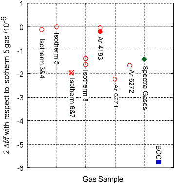
Figure 7. The observed variability of the speed-of-sound squared in argon compared with gas used in Isotherm 5. The data were estimated by measuring the resonant frequency of the (0, 3) resonance with the gas close to the temperature of the triple-point of water and at a pressure of 200 kPa. The graph shows twice the fractional shift in the resonant frequency expressed as parts in 106. Plotting the data in this way means the vertical axis is equivalent to the fractional change in molar mass of the gas.
Download figure:
Standard image High-resolution imageThe open red circles show data from Air Products BIP argon. The observed changes are equivalent to a range of 2.3 parts in 106 in M/γ. The green diamond shows data for Spectra Gases Spectra Grade gas imported from the USA. The blue square shows gas from BOC 6N grade gas and has an equivalent shift of 5.8 parts in 106 in M/γ.
At first we did not understand the origin of this variability and we checked for several possible effects. We observed no variation of
between gas sampled from a full bottle and the same bottle when it was nearly empty. The abbreviation 'BIP' stands for built-in purifier—a molecular sieve built into the outlet valve of the gas cylinder. To check for possible isotopic fractionation effects, Ar 4193 was first measured directly (open circle) and then after being decanted into a separate bottle (filled circle), leaving 30 min for isotopic equilibration. The small difference observed is close to the uncertainty of measurement and is clearly not the origin of the observed variability.
We tackled the possibility of chemical contamination by installing a cold trap, replacing the getters, and adding an additional large capacity cold getter and particle filter (SAES Microtorr MC1902F). None of these steps affected the observed frequency beyond the change detection-limit of 0.1 parts in 106. The gas used in Isotherms 6 and 7 was then subject to a mass spectroscopic examination at SUERC (table 2) and the molar mass of the gas was found to be heavier than the gas used in Isotherm 5 by 1.97(17) parts in 106. The expected shift in resonant frequency is shown as a cross on figure 7 and coincides almost exactly with the measured shift in 2Δf/f of 2.0(1) parts in 106. Further studies will be undertaken in due course, but we consider that this convincingly explains the observed variability in the speed of sound as being solely due to isotopic variability.
This observation supports previous reports of isotopic variability in argon [15, 24]. The similarity of the isotopic ratios of gas from Isotherms 3 and 4 and Isotherm 5 is not a coincidence. Investigation revealed that the bottles have the same 'batch number' and so are likely to have been filled at nearly the same time from gas with similar composition. The fact that independent measurements of their molar masses differ by only 0.01 parts in 106 suggests that the estimated type A uncertainty of the ARGUS mass spectrometer of uR = 0.169 × 10⁻⁶ may be conservative.
2.1.7. Overall estimate of uncertainty in molar mass.
Our measurements have found no evidence for impurity gases which might significantly affect the molar mass. So our overall uncertainty in (M/γ) is uR(M/γ) = 0.390 × 10⁻⁶, the quadrature sum of the terms arising from isotopic measurements uR = 0.390 × 10⁻⁶ and the detection limits of other impurity gases uR = 0.022 × 10⁻⁶ (table 5).
Table 5. Uncertainty contributions to the estimate of the molar mass M and the ratio M/γ.
| uR(M) ×10−6 | uR(M/γ) ×10−6 | Comment | |
|---|---|---|---|
| Isotopic | 0.390 | 0.390 | SUERC |
| Noble gases | 0.020 | 0.020 | GC-MSD measurements |
| Non-noble gases | 0.002 | 0.002 | Gas and getter specification |
| Water | 0.055 | 0.008 | Trace moisture measurements |
| 0.390 | Quadrature sum | ||
2.2. Temperature
2.2.1. Introduction.
Our link to the current SI definition of temperature is through realization of TTPW and the calibration of six capsule standard platinum resistance thermometers (PRTs) at that temperature. The two TPW cells used for this work were compared with NPL's reference TPW cells in November 2009 and the realized temperatures differed from the mean value of the reference cells by +10(42) µK and +9(42) µK. One of the cells used in this work was also compared with cells from across Europe in February 2010 and was 31(50) µK above the CCT-K7 key comparison reference value [30].
Electrically, the measurement of a PRT with uncertainty below 1 mK is challenging: for a measuring current of 1 mA and a resistance of 25 Ω, the voltage signal is 25 mV. For an uncertainty of 0.1 mK this must be determined with a resolution below 10 nV. To minimize transfer uncertainty between the calibration condition and the measurement, we used the same standard resistors and resistance bridge (ASL F18) for calibration and experimental measurements. Additionally the thermometers were transferred from the TPW cell directly into the apparatus without the disconnection of even a single electrical lead. This procedure significantly reduces measurement uncertainty because any error in the calibration caused by (say) an error in the estimated resistance of the standard resistor, or some aberrant behaviour of the bridge, will be automatically compensated in the measurement condition.
2.2.2. Thermal gradient.
With no power dissipated in the resonator, we found that the resonator was—as expected—nearly isothermal with temperature differences between thermometers of at most 20 µK. However the dissipation of microwave power warmed the equatorial thermometers (PRTs 3 and 4) relative to the neck thermometer PRT 1 by 77(10) µK and dissipation in the acoustic pre-amplifier caused a further warming of 280(10) µK and also gave rise to a temperature gradient across the resonator. The estimated uncertainty of 10 µK is a bridge reading uncertainty and is used in all estimates of temperature differences in this section to distinguish between experimental and model 'measurements', which are shown without an uncertainty indication
After acoustic measurements were completed, the pre-amplifier dissipation was estimated to be approximately 1.7 mW by measurements of the dc current consumption and voltage. Using this as a gauge allows us to estimate the likely microwave dissipation as ∼0.5 mW, which may be compared with the dissipation due to the thermometers of 6 × 25 µW = 0.15 mW.
To improve our understanding of the heat flow through the resonator, we constructed a simplified thermal model in Comsol (figure 8). Temperature differences were estimated using 1000 times the nominal heat flux (1.7 W instead of 1.7 mW) in order to improve the stability of the numerical solution. The heat sources were modelled as 1.7 mW dissipated in a stainless steel cylinder attached to the sphere in the same location as the preamplifier, and 0.5 mW uniformly distributed across the inner surface of the sphere. The model considered the effect of gas within the resonator, but neglected gas outside the resonator, the holes in the flanges and the thermal impedances at mating surfaces.

Figure 8. The results of modelling the temperature gradients within the sphere. (a) A 3D model showing the location of the thermometers and the pre-amplifier. Modelled temperatures are shown as differences from the mean inner-surface temperature in microkelvin. (b) The model results for the inner surface of the resonator. (c) An unfolded map of the inner surface showing the hot spot and the pole-to-pole gradient. Note that this presentation exaggerates the area of regions near the north and south poles. (d) Graph showing more fairly the model results for the distribution of surface temperatures on the inner surface of the resonator, and the distribution of temperatures within the gas. Also shown is the model expectation for the results from the equatorial thermometers PRTs 3 and 4.
Download figure:
Standard image High-resolution imageThe model describes the temperature gradients within the resonator only within a factor 2 (table 6). So for example the measured difference between the equatorial thermometers (PRTs 3 and 4) and 'south pole' thermometers (PRTs 5 and 6) was 91(10) µK compared with a model estimate of 65 µK. This difference might reflect small differences in the structure around the pre-amplifier. Similarly, the difference between the equatorial thermometers (PRTs 3 and 4) and 'neck' thermometer (PRT 1) was measured to be 357(10) µK compared with a model estimate of 186 µK. This extra temperature difference could possibly have arisen from the mating surface between the neck and the sphere. This was a copper–copper junction with one surface diamond-turned and the other conventionally machined, but no thermal paste was used. Nonetheless, despite its shortcomings, we consider the model to be useful in interpreting the experimental data.
Table 6. Modelled and measured temperature differences (in microkelvin) within the sphere shown as shifts from the average of the equatorial thermometers. The lower two rows show the modelled differences between the equatorial thermometers. PRT 2 was used a control thermometer and so its temperature was not recorded.
| n | Model | Measured | |
|---|---|---|---|
| Neck | 1 | −186 | −357(10) |
| Equator | 3 & 4 | 0 | 0 |
| South pole | 5 & 6 | +65 | +91(10) |
| Average over inner surface | +10 | ||
| Average of gas | +10 |
For example, experimentally we noted that when power is dissipated within the resonator the temperature difference between the neck thermometer PRT 1 and the equatorial thermometers (PRTs 3 and 4) was larger than the temperature difference between the equatorial thermometers and the 'south pole' thermometers (PRTs 5 and 6). This can be understood qualitatively in terms of the cross-sectional area of copper through which the heat must flow to leave the resonator, and the model also reproduces this behaviour.
The model predicts that PRT 1 should be approximately 90 µK hotter than the 'north pole' on the inner surface—and so it is only a poor indicator of the 'north pole' temperature. In contrast the model predicts that PRTs 5 and 6 should be 4 µK cooler than the temperature of the inner surface at the 'south pole'. And significantly, the model predicts that PRTs 3 and 4 differ by only 10 µK from the average temperature of the entire inner surface of the resonator which is also (within 1 µK) equal to the volumetric average temperature of the gas within the resonator. The model thus informs our choice of basing our central estimate of the gas temperature on the average of the equatorial thermometers, PRTs 3 and 4.
The model also allows us to estimate the distribution of temperatures across the inner surface of resonator and also within the gas (figure 8). Because PRT 1 in the neck is only a poor indicator of the temperature at the 'north pole' of the inner surface, we have chosen to estimate the range of temperatures within the sphere as twice the temperature difference between the equatorial thermometers (PRTs 3 and 4) and the south-pole thermometers (PRTs 5 and 6). As we mentioned above, the model predicts this difference should be 65 µK and the experimental difference is 91(10) µK.
Figure 8(c) shows the modelled distribution of temperature across the inner surface of the surface of the sphere. It is clear that there is a 'hot spot' near the microphone where the temperature exceeds the average temperature of the sphere by up to 143 µK. The region in excess of 100 µK corresponds to an area of approximately 16 mm radius around the microphone plug, and so corresponds to approximately 1.6% of the inner surface area. If we model the volume of gas heated by this area as a hemisphere of radius 16 mm, then this corresponds to approximately 0.3% of gas within the resonator. In fact the thermal model indicates that the heated volume is not quite so large.
Figure 8(d) shows the distribution of temperature sampled fairly over the inner surface of the sphere, and also from within the volume of gas in the sphere. In the model 95% of the inner surface of the resonator is within ±86 µK of the mean temperature, a distribution which may be characterized as approximately normal with a standard deviation of 41 µK. Volumetrically, 95% of the gas is within ±63 µK of the mean temperature, a distribution which may be characterized as approximately normal with a standard deviation of 31 µK.
Although the temperature gradient is larger than we would have planned, we consider that neither the 'hot spot' nor the gradient are likely in themselves to affect the inference of
. The TBL is negligibly affected by temperature deviations at this level, and because the propagation equations for sound are linear for these sub-part-per-million deviations, we expect that the resonant frequencies will closely reflect the average temperature of the gas. Experimentally we consider that the main consequence of the gradient is to introduce an additional uncertainty reflecting possible differences between the average gas temperature and the temperature of PRTs 3 and 4. Based on the experimental 91(10) µK difference between the equatorial thermometers (PRTs 3 and 4) and the south-pole thermometers (PRTs 5 and 6) we consider it likely that the mean gas temperature must lie in the range ±91 µK about the average of the equatorial thermometers (PRTs 3 and 4). If we model this as a range of uniform probability this results in an additional uncertainty component u(T) = 53 µK. We consider this a relatively conservative estimate, even given the shortcomings of the thermal model.
The overall uncertainty of the temperature is estimated as the quadrature sum of eight terms (table 7) with the four dominant contributions being: the realization of the TPW (42 µK), the overall temperature calibration uncertainty (65 µK), the effect of the temperature gradient across the resonator (53 µK) and the correction of the thermometer readings for self-heating (29 µK). Our final standard uncertainty is u(TTPW) = 99 µK (uR(TTPW) = 0.364 × 10⁻⁶).
Table 7. Uncertainty contributions to the estimate of the temperature.
| Temperature | /mK | uR/10−6 | Comment |
|---|---|---|---|
| Realization of TPW | 0.042 | 0.154 | International and national comparisons |
| Temperature calibration | 0.065 | 0.238 | From calibration certificate |
| Calibration drift | 0.011 | 0.040 | Estimated from differences between thermometers with acoustics and microwaves off |
| Bridge reading | 0.010 | 0.037 | SD ∼ 0.03 mK: Standard error of averaged bridge output |
| Gas temperature | 0.053 | 0.194 | Estimated from gradients in operating condition |
| Correction to TPW | 0.001 | 0.004 | Experiments generally within 1 mK of TPW |
| Self-heating correction | 0.029 | 0.106 | Extrapolation to 0 mA |
| Standard resistor stability | 0.010 | Estimated from resistor calibration history | |
| 0.099 | 0.364 | Quadrature sum | |
2.3. Equivalent radius
2.3.1. Surface perturbations.
We need to estimate the radius aeq seen by the acoustic sound field in the experimental configuration, i.e. with tubes carrying gas in and out of the resonator, with microwave antennas and with acoustic transducers. To achieve this we monitored the microwave spectrum as we inserted the acoustic transducers. Our estimate of aeq involves four key measurements summarized in figure 9 and described in detail below. These measurements show how estimates of aeq inferred from different microwave modes varied as we inserted acoustic transducers into the resonator.
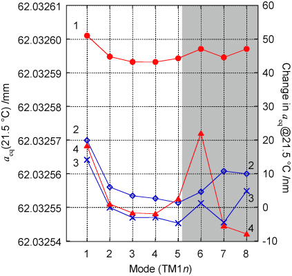
Figure 9. Estimates of the radius aeq at around room temperature deduced from eight TM1n modes as acoustic transducers and microwave antennas are modified in four stages described in the text. Measurements were taken in vacuum at several temperatures close to room temperature, but for the purposes of comparison they have been adjusted to show the value expected at 21.5 °C.
Download figure:
Standard image High-resolution imageMeasurement 1. In this measurement the resonator has two microwave probes and a gas evacuation line. We estimated aeq from each of the eight detectable TM microwave modes below 20 GHz. The maximum difference between the eight estimates for aeq in vacuum is 7 nm (u = 2.6 nm) (figure 9—label 1). This level of agreement arises from the exceptionally perfect realization of the resonator shape.
Measurement 2. Two blank plugs were removed and replaced with the plugs modified to accept acoustic transducers. Upon re-insertion, the difference in plug protrusion produced a small local deviation from the ellipsoidal form. From the change in the microwave frequencies, we estimated the change in aeq was Δaeq = −42 nm (figure 9—label 2).
Prior to assembly—when we still had access to the inner surface of the resonator—we had measured the volume perturbation caused by the imperfect fit of the acoustic transducer plugs. We did this using a quick-setting silicone compound to create a negative impression of the plug and the surrounding copper surface (figure 10). Using a confocal microscope to examine the moulding we estimated a volume change to be equivalent to Δaeq = −32(10) nm, consistent with the microwave result.
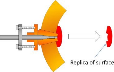
Figure 10. Illustration of how the perturbation caused by protrusion of the acoustic transducers was measured using a quick-setting silicone compound.
Download figure:
Standard image High-resolution imageMeasurement 3. The plugs carrying the acoustic transducers were withdrawn and replaced. With the exception of TM17, the resulting radius estimates (figure 9—label 3) were within approximately 5 nm of measurement 2. This allowed us to assess the reproducibility with which the transducers could be inserted. The origin of the anomalous change in the TM17 is discussed below.
Measurement 4. The plugs carrying the microwave probes were then removed and the volume around the bare-wire antennas filled with epoxy resin to ensure the equivalence of the microwave and acoustic volumes (figure 9—label 4). Aside from the TM16 mode, the radius estimates were mostly in agreement with measurement 3, confirming both the positional reproducibility of the plugs and the correction applied for the epoxy filling. The magnitude of this correction was 4 nm for the TM11 mode, and less than 1 nm for the other modes.
At the level of parts in 107 the microwave resonant frequencies can be perturbed by surface effects within the resonator, interference from neighbouring non-triplet modes, and resonances in the cable and the connectors. The observed dispersion (figure 9—label 4) is not caused by random noise, but is characteristic of the configuration of the resonator and its associated cables. As we have noted previously [11] surface perturbations affect TM11 modes more strongly than higher TM1n modes. However, at higher frequencies, the shorter wavelength of the microwaves results in a high density of standing-wave modes, in both the cable and connectors, and within the resonator itself. These can resonantly couple to the cavity at specific frequencies, causing spurious perturbations. These perturbations can be easily detected because they affect each component of a triplet differently—both in terms of its frequency and its half-width. So, for example, by considering the spacing of the modes within the triplet—which affects estimates of the geometrical parameters  1 and 2—it is possible to detect whether a radius estimate has been spuriously affected. These spurious interferences are the responsible for the anomalous high frequency results shown in traces 3 and 4 of figure 9.
When measured in the cryostat rather than a test vessel, the microwave cables are longer and attenuation is increased at higher frequencies, degrading the high-frequency signal-to-noise ratio. For these reasons we estimated aeq with the acoustic transducers inserted using the average of the TM12 to TM15 modes, which have a standard deviation of 2.0 nm. If we include the TM11 mode in the average, the estimate for aeq is shifted by 5 nm, and we use this to evaluate the uncertainty associated with the variation of aeq with mode. The effect of including or excluding the TM11 mode is included in the uncertainty assessment (table 8).
Table 8. Uncertainty contributions to the estimate of the equivalent radius.
| aeq | /nm | uR/10−6 | Comment |
|---|---|---|---|
| Statistical | 0.3 | 0.005 | From the intercept of aeq versus pressure |
| Acoustic transducers | 2.0 | 0.032 | Standard deviation of five modes |
| Acoustic transducers | 5.0 | 0.081 | Shift on inclusion of TM11 |
| Frequency reference | 0.0 | 0.000 | Rubidium clock was stable to 1 part in 109 |
| Resonance fitting | 1.0 | 0.016 | Estimated from covariance |
| Surface conductivity | 2.5 | 0.040 | Uncertainty in skin depth as discussed in [11] |
| Waveguide correction | 7.2 | 0.116 | Perturbation by waveguides as discussed in [11] |
| Dielectric layer | 7.0 | 0.113 | Estimated maximum thickness [11] |
| 11.712 | 0.189 | Quadrature sum | |
Our radius estimate together with its overall uncertainty is shown in figure 11 in comparison with the microwave data from which it was derived.

Figure 11. The radius estimated in vacuum from each of the TM11 to TM15 mode triplets. The values are shown together with our best overall estimate of aeq(P = 0) and overall standard uncertainty u(aeq) = 11.7 nm (table 8).
Download figure:
Standard image High-resolution image2.3.2. Dielectric corrections for argon.
The steps described in section 2.3.1 are relevant to determining the radius of the resonator in vacuum. Microwave measurements were made throughout all the isotherms which allowed estimates of aeq to be made as a function of gas temperature and pressure. However determining aeq requires compensating for the frequency shift arising from the dielectric constant of argon [31]. This correction is large—approximately 274 parts in 106 for a gas pressure of 100 kPa—and so amounts to approximately 1918 parts in 106 for a gas pressure of 700 kPa. To correct for this requires knowledge of the gas density which is estimated from independently acquired pressure and temperature data and the known virial coefficients and dielectric constant for argon. If the pressure is estimated incorrectly then the apparent radius will show anomalous variations [21].
Figure 12 shows the corrected radius estimate as a function of pressure. The data are clearly linear with residuals (figure 13) on the order of 1 nm. These results correspond to measurements taken over three months during which the resonator was cycled in pressure. It is clear that the resonator is remarkably dimensionally stable. The residuals also allow us to estimate how wrong our pressure measurements could be.

Figure 12. Estimates of the equivalent radius aeq at TTPW measured during Isotherms 3, 4 and 5.
Download figure:
Standard image High-resolution image
Figure 13. The residuals of a linear fit to the estimated radius as a function of pressure, aeq(P) shown in figure 12. The data were acquired over a period of three months during several pressure excursions over the entire pressure range. The residuals can be interpreted as either a radius error (left-hand axis) with a standard uncertainty of 1.1 nm or a pressure error (right-hand axis) with a standard uncertainty of 6.3 Pa. The data point at 0 Pa corresponds to a measurement made in vacuum and so has no dielectric correction. The shaded band shows the estimated range of possible pressure errors based on our traceable pressure calibration.
Download figure:
Standard image High-resolution imageOur Ruska 7000 pressure indicator was calibrated before and after these experiments against a pressure balance with a relative standard uncertainty of uR ∼ 3 × 10⁻⁵ (∼3 Pa at 100 kPa and ∼21 Pa at 700 kPa). On recalibration after this work, the table of corrections showed changes of less than 10 Pa at all pressures. To eliminate drift of the pressure indicator during the experiments, it was re-zeroed against a turbo-molecular pump at each new pressure setting. After correction for the aero-static head, this gives us a traceable pressure measurement in the volume outside the resonator. To obtain the pressure measurement within the resonator we applied a correction based on measurements of changes in dielectric constant as a function of gas flow.
If our pressure estimate exhibited an offset then the extrapolation of the pressure data in figure 12 (aeq = 62.010 539 8 mm) would not fall close to the zero pressure datum taken in vacuum—i.e. P < 10 Pa. Similarly, if our pressure estimate exhibited a non-linear error, the residuals to a straight-line fit would not be randomly distributed. Re-casting the residuals as being due to pressure errors (figure 13 right-hand axis) we can eliminate the possibility of any non-linear errors in pressure measurement, and find the dispersion is characterized by a standard deviation of 6.3 Pa, consistent with our pressure calibration. As mentioned in section 1.2.8, this is of particular significance at low pressures, in ensuring that the TBL correction to the acoustic resonant frequencies is made correctly and consistently between different isotherms taken several months apart.
The contraction of 2.3 parts in 106 seen in figure 12 is approximately 25% greater than would be expected from the compressibility of the copper walls of the resonator. The difference could arise because our resonator is a composite object, or because the dielectric constant of argon is in error by approximately 3 parts in 104. In either case, it makes no difference to our estimate of
, but would be a small additional source of uncertainty in estimating the virial coefficients of argon.
2.3.3. Summary.
The overall uncertainty in the radius was estimated as the quadrature sum of eight terms (table 8). The three dominant contributions were: uncertainty in the correction for the microwave antennas (7.2 nm), the dispersion of radius values caused by inserting the acoustic transducers (5.0 nm) and the uncertainty in the effect of dielectric surface layers (7.0 nm).
2.4. Speed of sound
2.4.1. Introduction.
Our estimate of the limiting low-pressure speed of sound is deduced using data from Isotherms 3, 4 and 5. For each isotherm we held the temperature close to TTPW as we reduced the pressure from 700 kPa to 100 kPa in 50 kPa steps. At each pressure we made 10 measurements of the (0, 2) to (0, 9) acoustic resonances with a gas flow of 7.4 × 10⁻⁷ mol s−1 (1 sccm) through the resonator. After the main measurements, we extended our study to the lower pressure range between 100 kPa and 30 kPa in 10 kPa steps, with increased data coverage at each pressure to reduce the statistical uncertainty.
Our experimental estimates
are deduced according to equation (4) by first correcting the resonant frequencies f(0,n) for known perturbations, then dividing by the appropriate eigenvalue ξ(0,n), then multiplying by the estimated radius aeq(P).
The speed of sound in argon depends on pressure through non-linearities in the dependence of gas density on pressure. The virial equation of state predicts a polynomial dependence of
 with pressure [13] which we curtail at order 3 due to the small size of higher-order terms in this pressure range. However, the experimental estimates
derived from the resonator display a more complex pressure dependence.
with pressure [13] which we curtail at order 3 due to the small size of higher-order terms in this pressure range. However, the experimental estimates
derived from the resonator display a more complex pressure dependence.
Firstly, the term linear in pressure (coefficient A1) depends not only on changes in gas density, but also on the interaction between the radially symmetric acoustic oscillations and the 'breathing' resonance of the shell of the resonator [6, 32] which occurs at approximately 14.2 kHz, between the (0, 6) and (0, 7) resonances. This introduces a mode dependence into the A1 terms from different (0, n) resonances. Neglecting the (0, 6) which is drastically broadened by the shell effect, the extent of the shell-induced variability in
 is approximately ±100 parts in 106 for modes (0, 2)–(0, 5) and (0, 7)–(0, 9). This amounts to approximately 5% of the 1980 parts in 106 due to the virial properties of argon. Moldover et al [13] used a maximum pressure of 500 kPa and a stainless steel resonator for which the shell correction is approximately 3 times smaller. For the (0, 2) to (0, 6) resonances Moldover was able to apply an analytical correction (amounting to 20 parts in 106 at most), removing the need to separately fit each mode. We chose to make the resonator from copper to enable precision fabrication, simultaneous precision microwave measurements and to benefit from the excellent thermal conductivity of copper. This has resulted in a concomitantly larger shell correction which must be 'fitted' rather than corrected for. Our modelling indicates that this does not affect estimates of
.
is approximately ±100 parts in 106 for modes (0, 2)–(0, 5) and (0, 7)–(0, 9). This amounts to approximately 5% of the 1980 parts in 106 due to the virial properties of argon. Moldover et al [13] used a maximum pressure of 500 kPa and a stainless steel resonator for which the shell correction is approximately 3 times smaller. For the (0, 2) to (0, 6) resonances Moldover was able to apply an analytical correction (amounting to 20 parts in 106 at most), removing the need to separately fit each mode. We chose to make the resonator from copper to enable precision fabrication, simultaneous precision microwave measurements and to benefit from the excellent thermal conductivity of copper. This has resulted in a concomitantly larger shell correction which must be 'fitted' rather than corrected for. Our modelling indicates that this does not affect estimates of
.
Secondly, the TBL correction contains a 'thermal accommodation' term which depends on the extent of the equilibration of argon molecules with the wall of the resonator. This cannot be predicted a priori but may be evaluated by fitting an additional A−1P−1 term [13, 15]. In order to arrive at a form to which we can fit the data, we note that over the limited pressure range of this work, the A3 term cannot be well estimated, and so before fitting our data, we subtract an estimate of the term derived from work at higher pressure [14, 33, 34]:

2.4.2. The effect of gas flow.
We chose to flow gas through the resonator so as to avoid possible outgassing effects on gas purity. Aside from a small change in pressure caused by the flow impedance of the tubes carrying gas in and out of the resonator we had not anticipated any flow-dependent effects. However Pitre et al [14] did observe an anomalous change in resonant frequencies as a function of flow and so we carried out an investigation (figure 14) and observed an effect similar in magnitude to that observed by Pitre et al [14]. However we observe an increase of frequency with flow while Pitre et al observe a decrease. We have not established any definitive cause of this effect, but we agree with Pitre (private communication) that it may be connected with the formation of vortices as the gas enters the resonator.

Figure 14. The effect on the frequency of the (0, 3) resonance at pressures of 300 kPa and 700 kPa shown relative to the minimum resonant frequency. The units of flow are standard cubic centimetres per minute (sccm) and 1 sccm = 7.4 × 10⁻⁷ mol s−1. The arrow shows the flow rate used in this work. We conclude that at 1 sccm, any frequency effect is negligible.
Download figure:
Standard image High-resolution imageAt a flow rate of 1 sccm the effect of flow is small, if not zero. Consequently we have chosen not to make a correction and also not to add an additional uncertainty component because the component (uR ∼ 0.02 × 10⁻⁶) would have a negligible impact on the overall uncertainty, changing
 by ∼0.001 × 10⁻⁶. Our experimental approach of using the lowest possible flow contrasts with Pitre et al [14] who used flow rates varying between 1 sccm and 60 sccm, using an empirical fitting function to estimate the zero-flow value.
2.4.3. Data reduction and fitting procedure.
We have adopted a fitting procedure which shows that the data are demonstrably consistent with the model assumptions. To achieve this we combined
data from Isotherms 3, 4 and 5 into a single data model. First, repeated measurements on a particular resonance at a particular pressure were averaged and the type A standard uncertainty calculated (figure 15). We then created a pooled relative standard uncertainty value
 based on the type A uncertainties to yield a single type A uncertainty applicable to every mode at a particular pressure. We then fit all the data to a single model as discussed in section 2.4.1.

Figure 15. The type A standard uncertainty of each mode at each pressure. In our analysis the pooled uncertainty (shown as a thick dotted line) was used. In order to obtain statistical consistency, the pooled uncertainty was inflated by a factor 2.28 (shown as a full line). The data are shown with the vertical axis scaled logarithmically for (a) all the data considered collectively, and (b) to (h) for each mode in turn, with data identified by isotherm.
Download figure:
Standard image High-resolution imageThe pooled estimate for
 was estimated as the square root of the average of the variances of each estimate for
at each pressure. As figure 15 shows, the pooled estimate of the type A uncertainties averages modes which have a low type A uncertainty with modes which have a higher type A uncertainty. Each individual type A estimate is derived from data taken over a few hours, but the pooled estimate is used to estimate the random variability of data taken several months apart. So it is not surprising that that
was estimated as the square root of the average of the variances of each estimate for
at each pressure. As figure 15 shows, the pooled estimate of the type A uncertainties averages modes which have a low type A uncertainty with modes which have a higher type A uncertainty. Each individual type A estimate is derived from data taken over a few hours, but the pooled estimate is used to estimate the random variability of data taken several months apart. So it is not surprising that that
 is an underestimate of the scatter of the data at a particular pressure, and needs to be 'inflated' to fairly describe the fit to the data. The pooled estimate changes abruptly at 100 kPa because at lower pressures we took more data, which reduces the standard uncertainty considerably.
Isotherms 3 to 5 each yield 13 data pairs P,
 for each of the (0, 2) to (0, 5) and (0, 7) to (0, 9) resonances, the (0, 6) data being excluded because of the strong shell interaction. In addition, after Isotherm 5 we acquired lower pressure data (30 kPa to 90 kPa in 10 kPa steps) from all resonances. After initial consideration, we also eliminated the (0, 5) data from all isotherms because on examining the residuals to initial fits, the (0, 5) residuals were clearly not normally distributed. The effect of this choice is discussed below. The residuals of an initial fit to the data (277 points) showed 14 anomalous data points. The 600 kPa data for all modes for Isotherm 5 (6 points) were eliminated because the wrong flow setting had been used. The low-pressure data from the (0, 7) resonance (5 points) were eliminated because the excess half-widths were too large due to interference from broadening of neighbouring modes. Additionally we removed a further three unexplained anomalous points.
Our final data set had 263 points and our model had nine free parameters. Using information provided by a chi-squared test, the pooled standard uncertainty was found to be too small to model the data, but when increased by a factor 2.28, 96% of the 263 points fell within ±2 standard uncertainties of the fit, indicating that the data are consistent with the model. The fit yielded an estimate of
with a relative standard uncertainty of
 , indicating a very high degree of self-consistency among the modes and between isotherms taken three months apart. The normalized residuals of fits to the data are shown in figure 16. Given that we chose to use a pooled uncertainty rather than a conservative value, this seems reasonable. However, it does indicate that other factors may be giving rise to some variability among the data.
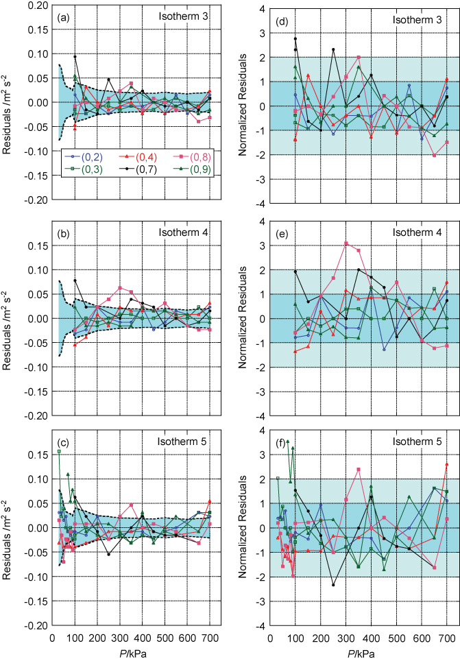
Figure 16. Residuals of the fit to the data using the parameters in table 9. The residuals from Isotherms 3, 4 and 5 are shown separately, but the fit has been made to all the data collectively. The legend in (a) applies to all panels. (a), (b) and (c) show the residuals in
and the inflated uncertainty estimate described in figure 15 is shown as a dotted line and a shaded band. (d), (e) and (f) show the residuals in
normalized to the inflated uncertainty estimate. The darker shaded band (±uR) corresponds to the shaded band in panels (a), (b) and (c). The lighter shaded band corresponds to ±2uR within which 96% of the residuals lie.
Download figure:
Standard image High-resolution imageTable 9 shows the parameters of the best fit to the data from Isotherms 3, 4 and 5. To assess the effect of uncertainty in the A3 term, the entire data analysis procedure was calculated twice, first with our central estimate A3 = 1.45 × 10⁻⁹ m2 s−2 kPa−3 subtracted from the data and then with a second estimate A3 = 1.20 × 10⁻⁹ m2 s−2 kPa−3 subtracted. This change increased the value of
by 0.213 parts in 106. However following Pitre et al [14], the uncertainty in A3 is smaller than this shift and is best estimated by the standard deviation of the three literature values [33, 34]: u(A3) = 0.09 × 10⁻⁹ m2 s−2 kPa−3. We thus scaled this shift by 0.09/0.25 to arrive at the concomitant uncertainty
 parts in 106.
Table 9. Column 1 shows the best fit parameters to our data set and their standard uncertainties. Columns, 2 to 5 show the effect of changing some parameters and refitting the dataset. The shifts in
(shown in parts in 106) are used to estimate the type B uncertainty to associate with each term (table 10). Column 2 shows the results of changing the A3 term from our central estimate of A3 = 1.45 × 10⁻⁹ m2 s−2 kPa−3 to A3 = 1.20 × 10⁻⁹ m2 s−2 kPa−3. Column 3 shows the results of changing the estimated thermal conductivity of argon λ to λ + u(λ). Column 4 shows the results of a revised estimate of the TBL correction recalculated with P + u(P). Column 5 additionally shows the effect of a worst case pressure error consistent with our calibration. This consists of a 6.3 Pa offset and linear error resulting in a pressure error of 13.5 Pa at 700 kPa. At the resolution shown, the addition of the linear term makes no difference to any of the terms in table.
| 1 | 2 | 3 | 4 | 5 | ||
|---|---|---|---|---|---|---|
| Central estimate | Effect of A3 uncertainty | Effect of thermal conductivity uncertainty | Effect of pressure offset | Effect of pressure offset + linear | Units | |
| Δλ | 0 | 0 | +u(λ) = 0.1% | 0 | ||
| ΔP | 0 | 0 | 0 | +u(P) = 6.3 | (6.3 + 1.02) × 10−5P | Pa |
| A3 | 1.45 × 10⁻⁹ | 1.20 × 10⁻⁹ | 1.45 × 10⁻⁹ | 1.45 × 10⁻⁹ | 1.45 × 10⁻⁹ | kPa−3 m2 s−2 |
| A−1 | 37.9(11) | 37.1(11) | 37.6(10) | 38.4(11) | 38.4(11) | kPa m2 s−2 |
|
|
94 756.245(17) | 94 756.265(17) | 94 756.229(17) | 94 756.235 (17) | 94 756.235(17) | m2 s−2 |
 |
0 | +0.213 | −0.169 | −0.106 | −0.106 | parts in 106 |
| A1(0, 2) | 0.221 588(65) | 0.221 449(65) | 0.221 627(64) | 0.221 628(65) | 0.221 628(65) | kPa−1 m2 s−2 |
| A1(0, 3) | 0.220 508(65) | 0.220 369(65) | 0.220 552(64) | 0.220 547(65) | 0.220 547(65) | kPa−1 m2 s−2 |
| A1(0, 4) | 0.217 721(65) | 0.217 583(65) | 0.217 768(64) | 0.217 761(65) | 0.217 761(65) | kPa−1 m2 s−2 |
| A1(0, 7) | 0.246 135(65) | 0.245 996(65) | 0.246 185(64) | 0.246 175(65) | 0.246 175(65) | kPa−1 m2 s−2 |
| A1(0, 8) | 0.234 000(65) | 0.233 861(65) | 0.234 051(64) | 0.234 040(65) | 0.234 040(65) | kPa−1 m2 s−2 |
| A1(0, 9) | 0.231 544(65) | 0.231 405(65) | 0.231 595(64) | 0.231 584(65) | 0.231 584 (65) | kPa−1 m2 s−2 |
| A2 | 5.0847(66) × 10−5 | 5.1179(66) × 10−5 | 5.0804(65) × 10−5 | 5.0809(66) × 10−5 | 5.0809(66) × 10−5 | kPa−2 m2 s−2 |
To assess the effect of our choice to exclude the (0, 5) data we reanalysed all the data including the entire (0, 5) dataset from Isotherms 3 to 5. No parameters were strongly affected and the estimate of
was increased by 0.10 parts in 106, within the standard uncertainty of 0.18 × 10⁻⁶. The (0, 5) resonance did not appear in any way anomalous during Isotherms 1 and 2, but the (0, 7) resonance did. We consider that the most likely explanation of this is that small mechanical modifications made to the resonator support after Isotherm 2 affected either the position of the main shell resonances or another 'parasitic' mechanical resonance.
From the A−1 term we estimate the thermal accommodation factor h = 0.777(13) using
where K = 0.254 26 Pa for a resonator of aeq = 62 mm. This value is typical of those reported in the literature [15].
From the six
 parameters we estimated the second acoustic virial coefficient of argon to be 5.438(12) cm3 mol−1 using the procedure described by Pitre et al [35] to subtract the effect of the shell. This is approximately 0.4% higher than Pitre et al's estimate of 5.4157(1) cm3 mol−1. The analysis estimates the shell breathing-mode frequency to occur at approximately 14.2 kHz.
2.4.4. Uncertainty in the TBL.
In our previous work [16] we estimated the sensitivity of estimates of
to type B errors in the estimation of the TBL. In that work we considered the effect on estimates of the TBL of errors in temperature, pressure, molar mass, radius, thermal conductivity, viscosity, the second and third virial coefficients of argon and their first and second derivatives with respect to temperature. A similar calculation for this resonator reveals that the only significant contributions to the uncertainty in the TBL correction arise from uncertainty in the thermal conductivity of argon, λ and the pressure P.
To estimate the impact of uncertainty in λ we re-estimated the correction due to the TBL for each mode and each pressure using values of λ which had been changed by one standard uncertainty. We estimated λ in the limit of zero pressure from the work of May et al [36] which has a relative standard uncertainty of 0.084%. Corrections for the pressure dependence were made using viscosity virial coefficients [37] leading to an overall relative uncertainty of u(λ) = 0.1% (figure 17). Refitting the modified dataset (table 9) resulted in a fractional change in our estimate of
of 0.169 parts in 106. Our estimate of λ was deduced in a similar manner to Pitre et al [14], but at 100 kPa our estimate (16.409(16) mW m−1 K−1) differs from the estimate of Pitre et al (16.419(4) mW m−1 K−1) by 0.01 mW m−1 K−1. This difference is within our uncertainty estimate but outside Pitre et al's uncertainty estimate. In addition to using an uncertainty estimate which is four times larger than Pitre et al's, we also estimate the sensitivity of
to changes in λ to be more than twice as large as Pitre et al.

Figure 17. The values of thermal conductivity used in the calculation of the TBL. The shaded band shows the range ±0.1%, our estimated uncertainty. Also shown is the value quoted by Pitre et al [14].
Download figure:
Standard image High-resolution imageTo estimate the impact of uncertainty in pressure we re-estimated the correction due to the TBL for each mode and each pressure using values of P which had been changed in two ways. The first change was an offset of u(P) = 6.3 Pa in line with the standard deviation of the data shown in figure 13. The second change was an offset plus a linear error derived from the table of corrections for the pressure meter, u(P) = (6.3 + 1.02) × 10−5p. This correction forms the boundary of the shaded region in figure 13. Refitting these modified datasets (table 9) resulted in fractional changes in our estimate of
of 0.106 and 0.106 parts in 106 respectively. Interestingly, to the number of significant figures shown in the table, the additional linear error in pressure had no effect on the fitted parameters. Our calculated sensitivity to pressure errors is 21 times larger than Pitre et al's.
From these changes in λ and P we estimate type B uncertainties (table 9) which we add in quadrature with the type A statistical uncertainty and A3 uncertainty estimates.
Our final estimate of the limiting low-pressure speed of sound squared in argon is
 with an overall relative uncertainty
 where the dominant term
 arises from uncertainty in aeq (section 2.3).
The fitting procedure is implemented in a Matlab script which reads data from an Excel spreadsheet. The spreadsheet and script file are available for downloading as supplementary material from stacks.iop.org/Met/50/354/mmedia.
2.4.5. Excess half-widths.
The TBL both shifts the frequencies of acoustic resonance, thus affecting our estimate of
, and also broadens them by an equal amount. So analysis of the half-widths (g) of the resonances provides a check on the TBL correction to the frequencies (f) [21]. Figure 18 shows the difference (Δg/f) between the experimentally measured half-widths (gExp/f) and the theoretical estimates (gTheory/f) plotted normalized to the resonant frequency.
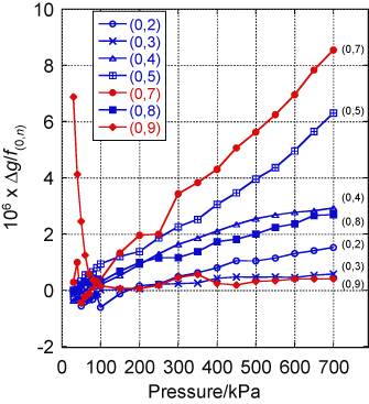
Figure 18. Difference Δg/f between experimental and theoretical half-widths of resonances from Isotherm 5 calculated using the second-order theory of Gillis [38] and expressed as a fraction of the resonance frequency, f. Notice that the (0, 7) and (0, 9) resonances have half-widths that increase rapidly at low pressure. These resonances were affected by broadening of nearby non-radial resonances. All the other resonances show a trend with extrapolations to zero within the uncertainty with which the theoretical half-width can be evaluated.
Download figure:
Standard image High-resolution imageThe low-pressure increase of the excess half-width for the (0, 7) and (0, 9) resonances is caused by the broadening of neighbouring non-radial resonances. The increase at high pressure is related to the interaction of the acoustic resonances with the shell resonance. The trend of the excess half-widths is to zero—within the uncertainty with which the half-width can be estimated.
We have evaluated gTheory using a theory correct to second-order in the ratio of the TBL to the radius [38]. This theory predicts a mode-dependent line-narrowing compared with first-order theory, but no shift in the resonant frequencies. Without the second-order correction, our data would appear to give a negative excess half-width, i.e. the acoustic line widths would appear to be narrower than predicted by the first-order theory.
The acoustic resonance line-widths are related to the dissipation of acoustic energy within the resonator. The fact that—in the limit of zero pressure—we have no excess line-width confirms that there are no unaccounted-for dissipative mechanisms operating in the resonator, at least within the uncertainty with which the theoretical half-widths may be predicted.
2.4.6. Summary.
Table 10 shows the three terms that contribute to the final estimate of the uncertainty in our estimate of the limiting low-pressure speed of sound squared,
. The dominant uncertainty is that due to uncertainty in the resonator size.
Table 10. Summary of the terms contributing to our uncertainty estimate for
.
|
|
/m2 s−2 | uR/10−6 | Comment |
|---|---|---|---|
| Statistical | 0.017 | 0.181 | k = 1 parameter uncertainty from fit |
 |
0.036 | 0.378 | 2 × Total aeq uncertainty |
| A3 uncertainty | 0.007 | 0.077 | Effect of u(A3) term from [31] or [32] |
| λ uncertainty | 0.016 | 0.169 | Effect of a thermal conductivity error of 0.1% |
| P uncertainty | 0.010 | 0.106 | Effect of a pressure offset of 6.3 Pa |
| 0.045 | 0.470 | Quadrature sum | |
2.5. Boltzmann constant
Our results from sections 2.1 to 2.4 are combined using equation (1) to yield estimates for R and kB. The relative standard uncertainty in R is estimated as the quadrature sum of the relative standard uncertainties in M,
and T. The standard uncertainty in kB additionally includes the standard uncertainty in NA (table 11). We find R = 8.314 478 7(59) J K−1 mol−1 which corresponds to kB = 1.380 651 56(98) × 10−23 J K−1. When restricted to two significant figures, both values have the same relative standard uncertainty uR = 0.71 × 10⁻⁶.
Table 11. Estimates of R and kB and associated uncertainty. The last column labelled 'weight' shows the percentage contribution of each term to the overall uncertainty.
| Estimate | uR/10−6 | Weight | ||
|---|---|---|---|---|
| M | g mol−1 | 39.947 816(17) | 0.390 | 30.0% |
| T | K | 273.160 000(99) | 0.364 | 26.1% |
|
|
m2 s−2 | 94 756.245(45) | 0.470 | 43.6% |
| R | J K−1 mol−1 | 8.314 478 7 (59) | 0.711 | |
| NA | mol−1 | 6.022 141 29 (27)×1023 | 0.044 | 0.4% |
| kB | J K−1 | 1.380 651 56 (98) × 10−23 | 0.712 | |
2.6. Uncertainty table
For convenience, all the component uncertainty tables for molar mass (table 5), temperature (table 7), equivalent radius (table 8) and speed-of-sound squared (table 10) are shown together in table 12.
Table 12. A combined uncertainty table. The 'weight' column shows the fraction of the overall uncertainty attributable to each component.
| Molar mass/gamma | Weight | uR/10−6 | Comment | |
|---|---|---|---|---|
| Isotopic type A | 5.6% | 0.169 | From the standard deviation of SUERC isotope ratios | |
| Reference to Lee et al | 24.3% | 0.351 | From the uncertainty in the estimation by Lee et al of the argon isotope ratios in air [28] | |
| Noble gas impurities | 0.1% | 0.020 | Based on GC-MSD measurements | |
| Non-noble gas impurities | 0.0% | 0.002 | Based on gas and getter specifications | |
| Water | 0.0% | 0.008 | Based on trace moisture measurements | |
| 30.0% | 0.390 | 0.3902 (Additional digits) | ||
| Temperature | Weight | /mK | uR/10−6 | Comment |
| Realization of TPW | 4.7% | 0.042 | 0.154 | International and national comparisons |
| Temperature calibration | 11.2% | 0.065 | 0.238 | From calibration certificate |
| Calibration drift | 0.3% | 0.011 | 0.040 | Estimated from differences between thermometers with acoustics and microwaves off |
| Bridge reading | 0.3% | 0.010 | 0.037 | SD ∼ 0.03 mK: Standard error of averaged bridge output |
| Gas temperature | 7.4% | 0.053 | 0.194 | Estimated from gradients in operating condition |
| Correction to TPW | 0.0% | 0.001 | 0.004 | Experiments generally within 1 mK of TPW |
| Self-heating correction | 2.2% | 0.029 | 0.106 | Extrapolation to 0 mA |
| Standard resistor stability | 0.0% | 0.010 | Estimated from resistor calibration history | |
| 26.1% | 0.099 | 0.364 | 0.3637 (Additional digits) | |
| aeq | Weight | /nm | uR/10−6 | Comment |
| Statistical | 0.0% | 0.3 | 0.005 | From the intercept of aeq versus pressure (figure 12) |
| Acoustic transducers | 0.8% | 2.0 | 0.032 | SD of five modes |
| Acoustic transducers | 5.2% | 5.0 | 0.081 | Shift on inclusion of TM11 |
| Frequency reference | 0.0% | 0.0 | 0.000 | Rubidium clock was stable to 1 part in 109 |
| Resonance fitting | 0.2% | 1.0 | 0.016 | Estimated from covariance |
| Surface conductivity | 1.3% | 2.5 | 0.040 | Uncertainty in skin depth as discussed in [11] |
| Waveguide correction | 10.6% | 7.2 | 0.116 | Perturbation by waveguides as discussed in [11] |
| Dielectric layer | 10.1% | 7.0 | 0.113 | Consequence of the use of TM modes only [11] |
| 28.1% | 11.712 | 0.189 | 0.1889 (Additional digits) | |
|
|
Weight | /m2 s−2 | uR/10−6 | Comment |
| Statistical | 6.5% | 0.017 | 0.181 | k = 1 parameter uncertainty from fit. |
|
|
0.036 | 0.378 | 2 × total aeq uncertainty | |
| A3 uncertainty | 1.2% | 0.007 | 0.077 | Effect of u(A3) term from [33] or [34] |
| λ uncertainty | 5.6% | 0.016 | 0.169 | Effect of a thermal conductivity error of 0.1% |
| P uncertainty | 2.2% | 0.010 | 0.106 | Effect of a pressure offset of 6.3 Pa |
| 15.4% | 0.045 | 0.470 | 0.4703 (Additional digits) | |
| Avogadro constant | /mol−1 | uR/10−6 | Comment | |
| NA | 0.044 | CODATA 2010 [5] | ||
| Overall | Weight | uR/10−6 | Additional digits | |
| M/γ0 | 30.0% | 0.390 | 0.3902 | |
| T | 26.1% | 0.364 | 0.3637 | |
|
|
43.6% | 0.470 | 0.4703 | |
| NA | 0.4% | 0.044 | 0.0440 | |
| Total R | 0.711 | 0.7111 | ||
| Total kB | 0.712 | 0.7125 | ||
3. Discussion
3.1. Comparison with previous work
3.1.1. Overall results.
In this section we refer to previous works using the labels used by CODATA [5]. Table 13 and figure 19(a) show our result alongside the previous two most accurate estimates of kB. Our estimate is 0.93 parts in 106 above the NIST 1988 value [13] but the difference is not statistically significant, being only half the standard uncertainty in the difference. Our result is 2.74 parts in 106 above the LNE 2011 value [14] and the difference is significant, being twice the standard uncertainty in the difference. Our result is 2.00 parts in 106 higher than the CODATA 2010 value [5] because the CODATA 2010 value is heavily weighted by the LNE 2011 result.
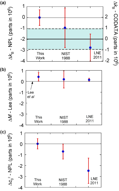
Figure 19. Differences in (a) kB, (b) M and (c)
between this work, NIST 1988 and LNE 2011. The vertical scale has the same magnitude for all graphs. (a) The final result with published uncertainty. The results are plotted as parts in 106 difference between (on the left-hand scale) our result and (on the right-hand scale) CODATA 2010 recommended values. The shaded band is the CODATA combined uncertainty at k = 1. (b) The molar mass estimates of the three works plotted as differences from the recommended values of Lee et al for atmospheric argon. (c) Estimates of
plotted as differences from this work.
Download figure:
Standard image High-resolution image
Table 13. Comparison of estimates of kB, M and
between this work, NIST 1988 and LNE 2011. The uncertainty in
for this work is from table 12, and the uncertainties in other works are from intermediate steps in their publications. LNE 2011 contains a small error in the reported value of
but the result has been checked with the author. The results are plotted in figure 19.
| This work | NIST 1988 | LNE 2011 | ||
|---|---|---|---|---|
| kB | J K−1/10−23 | 1.380 651 56 (98) | 1.380 6503 (25) | 1.380 6478 (171) |
| Fractional difference/10−6 compared to this work | 0.00(71) | −0.93(180) | −2.74(116) | |
| M | g mol −1 | 39.947 816(16) | 39.947 807(32) | 39.947 805(6) |
| Fractional difference/10−6 compared to Lee et al (21) | +0.40, +0.41(17) | +0.18(79) | +0.14 (15) | |
|
m2 s−2 | 94 756.245(40) | 94 756.178(65) | 94 756.011(110) |
| Fractional difference/10−6 compared to this work | 0.00(42) | −0.70(69) | −2.47(116) |
When comparing results which are all close to the limits of what is technically possible, it is important to consider not just the simple combination of component uncertainties, but also the overall robustness of conclusions against possible systematic effects. Each of the three kB estimates in table 13 (figure 19) is the result of combining estimates of the three factors in equation (1): T,
, M. In turn below we consider differences between our work and others in the estimation of these factors with particular focus on the cause of the difference between this work and that of LNE 2011.
All the works were carried out close to TTPW and used broadly similar techniques to transfer the TTPW to their apparatuses. To explain the difference between this work and LNE 2011 by a temperature error alone would require an error of 0.76 mK which is unlikely in either work. From the results for
and M (table 13, figures 19(b) and (c)) it is clear that the molar mass estimates are similar, but that the estimate for
from LNE 2011 is significantly lower than this work or NIST 1988.
3.1.2. Speed of sound.
Our combined microwave and acoustic measurements permit four distinct types of internal consistency checks in our estimate of
which increase the overall robustness of our conclusion [21].
Firstly, we estimate
by extrapolation of c2(P) data from six acoustic resonances varying in frequency from 3.6 kHz to 21.1 kHz. We thus span a wide range of systematic corrections, most notably that due to the TBL. The relative standard uncertainty associated with mode-to-mode variability of
is uR = 0.181 × 10⁻⁶, which indicates an exceptional level of self-consistency, approximately two times better than LNE 2011.
Secondly, the equivalent radius of the resonator, aeq, which is a key input to our estimate of
, is the result of an exceptional series of characterizations and checks. To explain a discrepancy between this work and LNE 2011 would require an error of approximately 1.35 parts in 106 or 85 nm on the radius compared with our uncertainty estimate of 11.7 nm. We consider such an error is inconceivable.
Thirdly, we used microwave resonances to additionally measure the dielectric permittivity of the argon gas, providing a self-consistency check on our pressure measurements meaning errors were unlikely to exceed u = 6.3 Pa, which reinforces our traceable calibration estimate of uR ∼ 3 × 10⁻⁵. In this way we avoided uncertainties arising from the pressure errors on the order of 100 Pa reported in LNE 2011. This is critical at low pressures where pressure-dependent corrections are largest.
The sensitivity of an individual estimate of
 from a single mode at a single pressure can be inferred from figure 4(b). But the sensitivity of
to such errors is difficult to assess analytically, because it depends in a non-linear fashion on the choice of modes used in the fit, the pressure range over which data are acquired, and the weighting of data from different pressures and modes. We are currently investigating the relative significance of these factors.
from a single mode at a single pressure can be inferred from figure 4(b). But the sensitivity of
to such errors is difficult to assess analytically, because it depends in a non-linear fashion on the choice of modes used in the fit, the pressure range over which data are acquired, and the weighting of data from different pressures and modes. We are currently investigating the relative significance of these factors.
Fourthly, the extent to which the experimental half-widths match the theoretically expected half-widths gives us an insight into the possibility of unexpected physics taking place within the resonator (section 2.4.4). Our agreement with the second-order theory of Gillis [38] rules out a wide range of possible confounding mechanisms that might affect our inference of kB. Both LNE 2011 and NIST 1988 reported positive excess half-widths on the order of 1 part in 106 when compared with first-order theory.
3.1.3. Molar mass.
Our estimate is the result of a campaign of measurements over two years involving measurements at NPL, SUERC [19] and Air Products Ltd, the supplier of our argon gas. The differences in molar mass (table 13, figure 19) between this work, NIST 1988 and LNE 2011 are small compared with the variability reported in the literature [15, 24, 27, 28]. We consider it unlikely that this could be the origin of the discrepancy, but our estimate does rely on the estimate of molar mass of atmospheric argon made by Lee et al [28]. If that estimate were to be revised then our estimate for kB would need to be adjusted accordingly.
3.2. Summary
The significant difference between this work and LNE 2011 stems mainly from a difference in the estimate of
, and the origin of this discrepancy is not currently understood.
Examination of the contributions to measurement uncertainty in kB (table 12) shows that the largest single component (24.3%) is the uncertainty of the molar mass of atmospheric argon. If techniques such as those used by Valkiers et al [14, 15, 24] had been used, or if a comparison of the molar masses against mono-isotopic 40Ar [13] had been undertaken, this could have been reduced considerably. In fact this measurement could still be made post hoc if resources became available. It is difficult to see how the temperature calibration uncertainties (11.2%) could be reduced significantly, but the temperature gradient (7.4%) could have been eliminated by more careful design. In the estimation of the radius, it is difficult to see how uncertainties in the waveguide correction (10.6%) could be easily reduced. The uncertainty associated with possible dielectric layers on the surface of the resonator (10.1%) could be further investigated by use of 'loop' antennas to exploit TE as well as TM modes.
Acknowledgments
This work was funded by the Pathfinder programme of the UK's Department for Business, Innovation and Skills and by the iMERA and EMRP joint research programmes of the European Union. The SUERC Noble Gas Laboratories are supported by NERC Services and Facilities. Neil Downie and Gordon Ferrier of Air Products assisted with multiple measurements of BIP argon. The authors are grateful to Gordon Edwards, Stephanie Bell, Martin Milton, Richard Brown and Richard Rusby for discussions, and to colleagues throughout NPL too numerous to mention individually. The authors are also grateful to Roger Read and Alan Heaume of Cranfield University for their work creating the inner surface of the NPL–Cranfield quasispheres. In addition this work has benefitted greatly from the kind cooperation of Laurent Pitre, Roberto Gavioso and Eric May. The authors are grateful to the referees whose comments have substantially improved the manuscript.