

Abstract
This study investigates the relationship between the peak temperature elevation and the peak specific absorption rate (SAR) averaged over 10 g of tissue in human head models in the frequency range of 1–30 GHz. As a wave source, a half-wave dipole antenna resonant at the respective frequencies is located in the proximity of the pinna. The bioheat equation is used to evaluate the temperature elevation by employing the SAR, which is computed by electromagnetic analysis, as a heat source. The computed SAR is post-processed by calculating the peak spatial-averaged SAR with six averaging algorithms that consider different descriptions provided in international guidelines and standards, e.g. the number of tissues allowed in the averaging volume, different averaging shapes, and the consideration of the pinna. The computational results show that the SAR averaging algorithms excluding the pinna are essential when correlating the peak temperature elevation in the head excluding the pinna. In the averaging scheme considering an arbitrary shape, for better correlation, multiple tissues should be included in the averaging volume rather than a single tissue. For frequencies higher than 3–4 GHz, the correlation for peak temperature elevation in the head excluding the pinna is modest for the different algorithms. The 95th percentile value of the heating factor as well as the mean and median values derived here would be helpful for estimating the possible temperature elevation in the head.
Export citation and abstract BibTeX RIS
1. Introduction
International safety guidelines and standards for protecting humans from radio frequency (RF) fields have been established by the International Commission on Non-Ionizing Radiation Protection (ICNIRP) (1998) and the IEEE International Commission on Electromagnetic Safety (ICES) (IEEE-C95.1 2006, IEEE-C95.1-2345 2014). The peak specific absorption rate (SAR) averaged over 10 g of tissue is used as a metric for localised exposures for frequencies up to 3 GHz in IEEE-C95.1 (2006) and 10 GHz in ICNIRP (1998). The limit for public exposure in unrestricted environments in both the standard and the guideline is 2 W kg−1, whereas the limit for occupational exposure in restricted environment is 10 W kg−1. In the guidelines and standards, the spatial-averaged SAR is used as a surrogate for the temperature elevation, which may induce physiological effects in and cause damage to humans after excessive exposure. Extensive studies have been conducted for temperature elevations in the brain and eye (Kojima et al 2004, van Rhoon et al 2013, Adibzadeh et al 2015b), and the effectiveness of SAR for human protection has been discussed (van Rhoon et al 2011).
There are several differences between the SAR metrics in the two international guidelines and standards (ICNIRP 1998, IEEE-C95.1 2006), although their scientific rationales are identical. Harmonisation exists among the international guidelines and standards at least in terms of the SAR averaging mass, as the IEEE revised the mass from 1 g (IEEE-C95.1 1999) to 10 g (IEEE-C95.1 2006). One of the rationales for this revision was that temperature elevations under the exposure limits in the brain (Van Leeuwen et al 1999, Wang and Fujiwara 1999, Bernardi et al 2000, Gandhi et al 2001, Hirata et al 2003, Hirata and Shiozawa 2003, Hirata et al 2006a) and the eye (Hirata et al 2000, Hirata et al 2002, Hirata 2005) were shown to be small using computer simulations in anatomically based human head models (IEEE-C95.1 2006). However, discrepancies between the two standards and guidelines are still observed in the applicable upper frequency and averaging schemes. In IEEE-C95.1 (2006), the frequency range between 3 and 6 GHz is considered as the transition range. Moreover, schemes for spatially averaging the SAR (including the shape of the averaging volume) are different in the two standards and guidelines, in addition to the handling of the pinna region.
Much attention has been paid to the effective frequency region where the peak value of the 10 g-averaged SAR is appropriate as a metric for estimating the local temperature elevation. After the current version of the IEEE standard was issued in 2006, this research topic was investigated by different groups using high-resolution human head models (e.g. Hirata and Fujiwara 2009, Laakso 2009, McIntosh and Anderson 2010). In particular, the spatial-averaged SAR over 10 g of tissue is a good metric for estimating the temperature elevation over the head for frequencies up to approximately 6 GHz (Hirata and Fujiwara 2009); in other words, the averaged SAR over 10 g is a surrogate for the temperature elevation as listed in WHO (2010). Different averaging masses are used in the regulations in some countries; e.g. 1 g used in United States (FCC 1997). The SAR averaged over a mass larger or smaller than approximately 10 g results in lower correlation with the temperature elevation (Hirata and Fujiwara 2009).
For frequencies higher than those mentioned above, the power density is currently used as a metric (ICNIRP 1998, IEEE-C95.1 2006). These frequencies (above 6 GHz) will be used in fifth-generation mobile communication and therefore are receiving much consideration. However, the averaging scheme of the power density is not well defined and is also inconsistent between the guidelines. Additionally, the temperature elevation in the human tissue has not been well evaluated in anatomically based models for frequencies higher than 6 GHz, except in a few studies (Laakso 2009, McIntosh and Anderson 2010). In these circumstances, verification of the applicability of the peak spatial-averaged SAR as a surrogate for the peak temperature elevation is of interest even at frequencies higher than 6 GHz.
In this study, different human head models are used for investigating the relationship between the peak spatial-averaged SAR and the peak temperature elevation in the frequency range of 1–30 GHz. In particular, six averaging algorithms for mass-averaged SAR are considered in order to obtain insight into this relationship for frequencies above 6 GHz. The averaging algorithms are selected on the basis of the description in the ICNIRP guidelines and the IEEE standard. It should be noted that the correlation between the spatial-averaged SAR and the temperature elevation is not considered voxel-by-voxel over the head, unlike in previous studies (Hirata et al 2008, Hirata and Fujiwara 2009); instead, spatial peak values for the spatial-averaged SAR and temperature are considered. Note that the uncertainty and variability for a specific product (e.g. mobile phone) have not been discussed in this study as the main purpose of this study is to discuss the appropriateness of the peak spatial averaged SAR as a metric for the temperature elevation in the international safety guidelines and standards; see their philosophy (e.g. ICNIRP 2002).
2. Model and methods
2.1. Head models
In this study, both simplified (multi-layer cubes) and realistic (MRI-based) anatomical models were considered. Specifically, a seven-layer model, consisting of the skin (1.5 mm), fat (1.5 mm), muscle (2.5 mm), skull (4.5 mm), dura (1.0 mm), cerebrospinal fluid (1.0 mm), and brain (sufficiently thick), was considered as the model of the head (Drossos et al 2000).
MRI-based human voxel models for different ages, genders, and races were considered as realistic anatomical models. This study employed the Japanese male model TARO and female model HANAKO (Nagaoka et al 2004). In addition, the European models of Virtual Family (Duke, Billie) (Christ et al 2010) and NORMAN (Dimbylow 1997) were considered. These models have a resolution of a few millimetres and are segmented into 51–80 anatomical tissues and organs. All the models were truncated at the bottom of the neck because the rest of the body does not affect the human interaction with the dipole antenna.
2.2. Electromagnetic dosimetry
The finite-difference time-domain (FDTD) method (Taflove and Hagness 2003) was used to conduct electromagnetic dosimetry on a human body exposed to microwaves emitted from a dipole antenna. The SAR is defined as

where |E| is the peak value of the electric field at position r and σ and ρ are the conductivity and mass density, respectively, of the tissue. The dielectric properties of the tissues were determined with a 4-Cole–Cole dispersion model (Gabriel et al 1996), where the upper frequency at which the measured data were considered is 20 GHz. As the frequency increased, the penetration depth of the electromagnetic wave decreased, indicating that most of the energy is absorbed in the skin layer at high frequencies. At a frequency of 20 GHz, the difference between the skin dielectric properties of the two research groups is a few percent, as summarised in Sasaki et al (2014). Note that the conductivity of the child tissue was assumed to be identical to that of the adult because the variation in human tissues is within a few percent across age (Wang et al 2006).
A major source of the computational error in the FDTD method is the discretization error, which depends on the ratio between the cell size and the wavelength in biological tissue. A well-known rule to suppress the numerical dispersion error in FDTD simulations is that the maximum cell size should be smaller than one tenth of the wavelength; the numerical error is less than 10% for the local 10 g averaged and the whole-body averaged SAR under this condition (Pickwell et al 2004, Dimbylow and Bolch 2007, Kühn et al 2009, Laakso 2009). The original resolution of TARO, HANAKO, and NORMAN is 2 mm. Thus, each voxel was further divided into 64 voxels with a resolution of 0.5 mm up to 10 GHz and into 512 voxels with a resolution of 0.25 mm above 10 GHz to keep the computational accuracy as high as possible. An in-house smoothing algorithm with manual editing was applied in order to maintain the reliability of the models (Nagaoka et al 2005). Similarly, the finest resolution of Duke and Billie is 0.5 mm and thus one cell was divided into 64 with a resolution of 0.25 mm for frequencies higher than 10 GHz. Even if we changed the resolution of the model resolution higher than 0.25 mm, almost identical results were obtained even at 30 GHz. Another factor affecting the numerical error is the reflection error of the absorbing boundary, but it is negligibly small as reported in previous studies (Lazzi et al 2000, Findlay and Dimbylow 2006, Laakso et al 2007, Kühn et al 2009). Our computational results are shown to be in good agreement with those by other research groups via inter-comparison (Dimbylow et al 2008).
2.3. Thermal dosimetry
The temperature in the human model is computed by solving the bioheat equation (Pennes 1948). This equation, which takes into account various heat exchange mechanisms such as heat conduction, blood perfusion, and electromagnetically induced heating, is represented by the following expression:

where T is the temperature of the tissue, TB is the blood temperature, C is the specific heat of the tissue, K is the thermal conductivity of the tissue, Q is the metabolic heat generation, and B is the term associated with blood perfusion. Furthermore, r and t are the position vector and time, respectively.
The temperature elevation due to handset antennas can be considered to be small enough that it does not activate the thermoregulatory response, because the temperature elevation at the SAR limit (2 W kg−1 for the general public) is less than 0.5 °C (<3 GHz) (Hirata and Fujiwara 2009). Additionally, the blood temperature is assumed to be spatiotemporally constant because the power absorption due to antennas (the typical output power of handset antennas is less than a few hundred milliwatts) is much smaller than the metabolic heat generation of a male adult (~100 W), resulting in a marginal body-core temperature elevation. Then, the blood temperature in (2) is simplified as constant ( = 37 °C). The boundary condition for (2) is given by

where H, Ts, and Te respectively denote the heat transfer coefficient, the surface temperature of the tissue, and the temperature of air (independent of the position). Samaras et al (2006) pointed out the weakness of the boundary condition (3) for the bioheat equation when applied to the human model with the stair-casing approximation. Improved algorithm for reducing computational error has been proposed (Neufeld et al 2007, Laakso 2009). Such an algorithm would be essential when calculating the temperature itself. However, that error marginally influences temperature elevation, as shown in Wang and Fujiwara (1999). Thus, we used the conventional formula.
The bioheat equation subjected to the boundary condition was solved to obtain the thermally steady-state temperature elevation. Thus, the left-hand-side term of (2) was assumed to be zero and all the right-hand-side terms were independent of t. The equation was discretised using a finite difference method and solved by applying the geometric multi-grid method (Laakso 2009). The following were the parameters of the multi-grid method: the number of grid levels was 6, with the resolution halved for each level; the thermal properties of each lower-resolution grid were the arithmetic averages of those of the higher-resolution grid; the pre- and post-smoothing operations consisted of four and one iterations, respectively, of the Gauss–Seidel method; and finally, the prolongation and restriction operations were full weighting and linear interpolation. The iteration was continued until the relative residual of the solution was less than 10−7.
The thermal parameters used in this study are the same as those in Hirata and Shiozawa (2003). These parameters were borrowed primarily from Duck (1990). Dominant factors affecting the temperature elevation for localized exposure is the blood flow rate (Hirata et al 2006a, Laakso and Hirata 2011). According to our recent study, the variation of the temperature elevation due to variability in the measured blood perfusion rate is ±20% for frequencies 1–3 GHz, gradually decreases with the increase of the frequency, and is ±10% at frequencies above 10 GHz (Ota et al 2014). The heat transfer coefficient between the skin and air and that between the eye surface and air were set to 5.0 and 15 W (m2 · °C)−1, respectively, which are the typical values at a room temperature of 23 °C (Fiala et al 2001).
Our computational scheme for thermal computation was in good agreement with measured results for human exposure to ambient heat (Hirata et al 2015) as well as small animals exposed to microwaves (Hirata et al 2006b, Hirata et al 2011). In addition, our computational results for handset antennas were in good agreement with those by other groups for frequencies below 3 GHz, as summarized in IEEE-C95.1 (2006) and plane wave exposure (Hirata et al 2013) in comparison with Bakker et al (2011).
2.4. Exposure scenarios
Figure 1 shows the exposure scenarios considered in this study. As shown in this figure, a separation distance of 15 mm was chosen from the closest model surface excluding the pinna and the half-wave dipole antenna. The reason the dipole antenna was chosen is that commercial communications systems for frequencies in the 6 GHz band or higher are currently not well established. In addition, the dipole antenna is often considered in human exposure standards; for example, WHO (2010) cites only one paper that derived the correlation between SAR and temperature elevation (Hirata and Fujiwara 2009). The lengths of the antenna were adjusted to 151, 76, 51, 38, 31, 25, 21, 17, 14, 13, 11, 8.5, 6.5, and 4.3 mm for 1, 2, 3, 4, 5, 6, 7, 8, 9, 10, 12, 15, 20, and 30 GHz, respectively, so that it would resonate at the corresponding frequencies. The positions of the centre of the dipole antenna relative to the pinna are shown in figure 1. For comparison, the output power of the antenna is taken as 1 W. Note that the typical output powers of the mobile terminals in a few GHz band are less than a few hundred milliwatts.

Figure 1. Positions of feeding points of the dipole antenna relative to the head. The black circle is defined as the reference position.
Download figure:
Standard image High-resolution image2.5. Dose metrics
As a metric for the dosimetric evaluation, the peak value of the SAR averaged over 10 g of tissue was considered in the international guidelines and standards (ICNIRP 1998, IEEE-C95.1 2006). The SAR averaging schemes in the standards and guidelines differ in three aspects: the number of tissues allowed in the averaging process, the shape of the averaging volume, and the inclusion or exclusion of the pinna in the averaging volume. Based on these differences, six algorithms for SAR averaging, labelled algorithms (I)–(VI), were then considered, and their properties are listed in table 1. When considering the cubic averaging shape (algorithms (I) and (II)), the algorithm specified in the IEEE C95.3 standard (2002) was applied to clarify the treatment of the air region and the pinna. The pinna is treated separately from the head (IEEE-C95.1 2006) with a basic restriction of 4 W kg−1, which is twice as large as the head and trunk and identical to that of the limbs. In contrast, no clear definition of the tissue number (stated to be contiguous) is provided in the ICNIRP guidelines (1998). Therefore, averaging algorithm (I) may correspond to that prescribed in the IEEE standard, whereas algorithms (IV) and (VI) correspond to the scheme in the ICNIRP guidelines. The peak temperature elevation in the pinna is not considered when algorithms (I), (III), and (V) are employed, because the SAR in the pinna is not considered.
Table 1. Considered averaging algorithm schemes for the SAR calculation.
| No of tissues | Ave. shape | Pinna | |
|---|---|---|---|
| (I) | Unlimited | Cube | Excluded |
| (II) | Unlimited | Cube | Included |
| (III) | One | Arbitrary | Excluded |
| (IV) | One | Arbitrary | Included |
| (V) | Unlimited | Arbitrary | Excluded |
| (VI) | Unlimited | Arbitrary | Included |
In this study, we mainly focused on the heating factor, which is defined as the ratio of the peak temperature elevation to the peak 10 g-averaged SAR.
2.6. Correlation between SAR and temperature elevation
When the peak temperature evaluation is considered at the thermal steady state, it is appropriate to express the approximate peak temperature elevation in the head or brain as

where SAR, ΔT, and α are the SAR averaged over 10 g of tissue (W kg−1), the peak temperature elevation estimated by the regression line (°C), and the slope of the regression line (°C · kg W−1) which corresponds to the heating factor, respectively, and are determined by using the method of least squares (Sachs 2012). Note that the intercept of the regression line is set to zero because there is no temperature elevation without microwave power absorption. To evaluate the effectiveness of the estimation scheme for the peak temperature elevation, the coefficient of determination R2 is introduced as
where ΔTi is the peak temperature elevation for the ith scenario,  is the mean value of ΔTi, and
  is the value of ΔTi estimated from the regression line.
In addition to the coefficient of determination, the coefficient of variation (CV) is introduced to discuss the variability of the heating factor at various frequencies. The coefficient of variation is defined as the ratio of the standard deviation of  to
to  .
.
3. Computational results
3.1. SAR and temperature elevation in TARO for different SAR averaging algorithms
Figure 2 shows the distributions of the SAR and temperature elevation at frequencies of 2 and 8 GHz. The dipole antenna is located at the reference position (black circle in figure 1) and oriented in the up–down (superior–inferior) direction. As shown in figure 2, the distribution of the temperature elevation is smoother than that of the SAR. The penetration depth of the temperature elevation is larger than that in the SAR. These differences are due to the fact that the heat diffusion length is larger than the penetration depth of the electromagnetic wave (Hirata et al 2006a, Samaras et al 2007), which is on the order of a few millimetres at these frequencies.
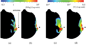
Figure 2. Distributions of SAR and temperature elevation in the head model of TARO resulting from dipole antenna. SAR at (a) 2 GHz and (b) 8 GHz, and temperature elevation at (c) 2 GHz and (d) at 8 GHz.
Download figure:
Standard image High-resolution imageFigure 3 shows the frequency dependence of the peak value of the SAR averaged over 10 g of tissue in TARO obtained using different averaging algorithms when the dipole antenna is located at position (e) and oriented in the up–down (superior–inferior) direction. As shown in figure 3, the different averaging algorithms yield different SAR tendencies, with the highest average SAR values appearing above 15 GHz for the cases in which the pinna is considered. This is because more than 60% of the power is absorbed around the pinna at frequencies higher than 7 GHz (see figure S1 (stacks.iop.org/PMB/61/5406/mmedia)). As the frequency increases, the penetration depth of the electromagnetic field decreases. The SARs computed with algorithms (III) and (V) and those with algorithms (IV) and (VI) are different at lower frequencies, but almost coincide with each other at frequencies higher than 12 GHz.
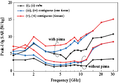
Figure 3. Peak SAR averaged over 10 g of tissue by different averaging algorithms.
Download figure:
Standard image High-resolution image3.2. Variability of heating factor in head models
In this section, the SAR and temperature elevation in five head models are computed for the dipole antenna located at the reference position in figure 1 and oriented in the up–down (superior–inferior) and front–back (anterior–posterior) directions; thus, 10 scenarios were considered for each frequency.
As shown in figures 4(a), (c) and (e), a comparison of the results of the anatomically based and multi-layer cube models using averaging algorithms (I), (III), and (V) reveals that the heating factors of the cube models are lower. The difference between the anatomically based and multi-layer models is more obvious for algorithms (III) and (V) than for algorithm (I). Figure 4 also demonstrates that the mean and median values of the heating factor peak at approximately 12 GHz for averaging algorithms (I) and (II) and approximately 6–10 GHz for the remaining algorithms. This broader frequency range may be attributable to the averaging shape of the SAR.
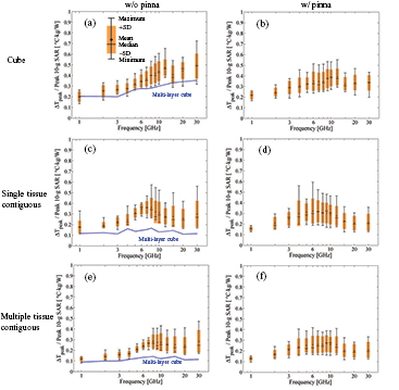
Figure 4. Heating factors for different human head models in the case of averaging algorithms (a) (I), (b) (II), (c) (III), (d) (IV), (e) (V), and (f) (VI). The antenna feeding position is the black circle in figure 1. The minimum, median, mean, and maximum values and the standard deviation of the heating factors are plotted.
Download figure:
Standard image High-resolution imageAs shown in figure 4(a), the median and mean values of the heating factor for averaging algorithm (I), which is similar to the averaging algorithm in the IEEE standard (IEEE-C95.1 2006), was rather flat (0.20–0.27 °C · kg W−1) for frequencies up to 4 GHz, and then it increased gradually with a further increase in frequency but became unstable at frequencies higher than 12 GHz. As can be confirmed from figure 5(a), a similar CV is observed for algorithm (II).

Figure 5. Coefficient of variation for different averaging algorithms with different (a) head models (antenna placed in the reference position) and (b) antenna feeding positions (TARO model).
Download figure:
Standard image High-resolution imageFigures 4(c) and (d) show the heating factors for averaging algorithms (III) and (IV), which permit any averaging volume shape but only a single type of tissue. One notable difference is the variability at 4 and 6 GHz in figure 4(d). It can be confirmed from figure 5(a) that the CV is largest at frequencies of 4 and 6 GHz. The CVs for algorithms (III) and (IV) are comparable to each other at frequencies higher than 10 GHz.
Figures 4(e) and (f) show the heating factor when any number of tissues is allowed in the averaging volume. As shown in figures 4(e) and (f), the tendencies of the heating factors are similar to those in the case of averaging algorithms (III) and (IV). However, the CVs of algorithms (V) and (VI) are smaller than those of algorithms (III) and (IV) at most frequencies.
At frequencies higher than 10 GHz, the CVs of algorithms (I) and (II) are smaller than those of algorithms (III)–(VI). The heating factors of algorithms (I) and (II) increase with increasing frequency for frequencies higher than 4 GHz.
3.3. Variability of heating factor in head models according to antenna position
Figure 6 demonstrates the effect of varying the antenna position (see figure 1) on the heating factor by using the head models Duke, TARO and NORMAN for averaging algorithms (I)–(VI). The reason for choosing these three models is that they are developed with different tissue classification algorithms. Comparing figure 6 with figure 4, similar mean and median values of the heating factors are observed in the two figures (see also figure S2). The antenna feeding point is a larger cause of variability in the heating factor than the model anatomy, which can be confirmed by comparing the respective CVs in figures 5(a) and (b). The variability becomes greater with increasing frequency. As with the case of model variability in section 3.2, the CVs of algorithms (I) and (II) are smaller than those of algorithms (III)–(VI) at frequencies higher than 10 GHz.
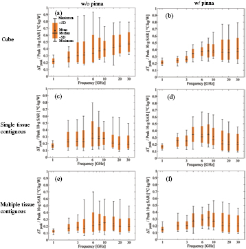
Figure 6. Heating factors and their variability with antenna positions in TARO and NORMAN for averaging algorithms (a) (I), (b) (II), (c) (III), (d) (IV), (e) (V), and (f) (VI). The minimum, median, mean, and maximum values and the standard deviation of the heating factors are plotted.
Download figure:
Standard image High-resolution image3.4. Heating factor statistics in different head models and at antenna positions
The statistical variation of the heating factor is discussed to give insight into the international standards and guidelines. At each frequency, we considered 40 cases: two polarizations in five head models at the reference point and 11 feeding positions (including the reference point) in three head models for vertical polarization. The upper frequency where the SAR is applicable is 3 GHz in the IEEE standard and 10 GHz in the ICNIRP guidelines. Thus, a total of 120 cases (40 cases at 1, 2, and 3 GHz) were considered for the former, whereas 280 cases (40 cases at 1, 2, 3, 4, 6, 8, and 10 GHz) were considered for the latter. As mentioned above, the intercept of the regression line was set as non-existent. All the data (up to 30 GHz, 400 cases) were considered when discussing the upper applicable frequency of the SAR. Similarly, in figure S4, the data of 200 cases (40 cases at 1, 2, 3, 4, and 6 GHz) were also plotted for frequencies up to 6 GHz, which is the upper transition frequency of IEEE.
As shown in figure 7, the R2 values for algorithms (I) and (V) are comparable to each other and show modest correlations (0.25 < R2 < 0.64) between the SAR and temperature elevation. On comparison, algorithm (V) shows a better R2 value than algorithm (III), suggesting that the inclusion of multiple tissues in the averaging volume provide better correlation. It can be expected from figure 5 that the CV for algorithm (V) is smaller than that for algorithm (III).
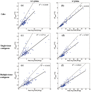
Figure 7. Relationship between the peak SAR averaged over 10 g of tissue and the peak temperature elevation for frequencies from 1 to 3 GHz for algorithms (a) (I), (b) (II), (c) (III), (d) (IV), (e) (V), and (f) (VI). The solid and dotted lines represent the regression line derived from the method of least squares and the line with the slope of the 95th percentile value of the heating factor.
Download figure:
Standard image High-resolution imageAs shown in figure 8, a modest correlation was observed between the SAR and temperature elevation for frequencies up to 10 GHz in comparison with algorithms (I), (III), and (V) where the SAR and temperature in the pinna are not considered. Strong correlations (R2 > 0.64) were observed between peak temperature elevation including the pinna and peak SAR with algorithms (II), (IV), and (VI), in which the SAR and temperature elevation in the pinna is considered, suggesting that the peak temperature elevation in the pinna can be estimated from the peak SAR when considering the pinna. Conversely, the SAR computed with algorithms (II), (IV), and (VI) may not be reasonably used to estimate the peak temperature elevation in the head excluding the pinna (see figure S3,); R2 was in the range between 0.0801–0.354.
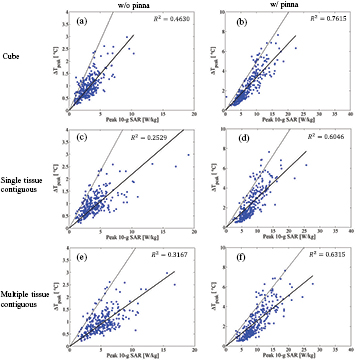
Figure 8. Relationship between the peak SAR averaged over 10 g of tissue and the peak temperature elevation for frequencies from 1 to 10 GHz for algorithms (a) (I), (b) (II), (c) (III), (d) (IV), (e) (V), and (f) (VI). The solid and dotted lines represent the regression line derived from the method of least squares and the line with the slope of the 95th percentile value of the heating factor.
Download figure:
Standard image High-resolution imageAs shown in figure 9, the values of R2, except for those of algorithms (III) and (V), became small when the data for frequencies from 1 to 30 GHz were considered. The decrease in R2 values in comparison with the case where the target frequency range was 1–10 GHz, except for the algorithms (III) and (V), is expected from figure 5 that the CVs at frequencies higher than 10 GHz are larger than those at lower frequencies. The increase in the R2 values in algorithms (III) and (V) may be coincidental, but the mean and median values of the heating factor are rather uniform in the frequency range considered herein.

Figure 9. Relationship between the peak SAR averaged over 10 g of tissue and the peak temperature elevation for frequencies from 1 to 30 GHz for algorithms (a) (I), (b) (II), (c) (III), (d) (IV), (e) (V), and (f) (VI). The solid and dotted lines represent the regression line derived from the method of least squares and the line with the slope of the 95th percentile value of the heating factor.
Download figure:
Standard image High-resolution imageThe 95th percentile values of the heating factor are listed in table 2 for the above three frequency ranges. By multiplying the values presented in this table and the SAR averaged over 10 g of tissue, the temperature elevation in the head can be conservatively estimated. The 95th percentile value of the heating factor at frequencies under 3 GHz was the lowest and increased when the target frequencies extended to 10 and 30 GHz. This is because the SAR concentrates around the antenna due to both the shallower penetration depth of electromagnetic waves and smaller antenna dimensions, and thus the SAR averaged over the volume of 10 g of tissue may not be sufficient.
Table 2. 95th percentile value of the heating factor for different averaging algorithms and frequency ranges.
| Frequency range | Algorithm | 95 percentile value of the heating factor |
|---|---|---|
| 1–3 GHz | (I) | 0.4264 |
| (II) | 0.3249 | |
| (III) | 0.4515 | |
| (IV) | 0.3530 | |
| (V) | 0.2677 | |
| (VI) | 0.2835 | |
| 1–10 GHz | (I) | 0.5677 |
| (II) | 0.4934 | |
| (III) | 0.4675 | |
| (IV) | 0.4877 | |
| (V) | 0.3784 | |
| (VI) | 0.4008 | |
| 1–30 GHz | (I) | 0.6564 |
| (II) | 0.5114 | |
| (III) | 0.4621 | |
| (IV) | 0.4948 | |
| (V) | 0.3809 | |
| (VI) | 0.4159 | |
3.5. Heating factor in the brain of different head models
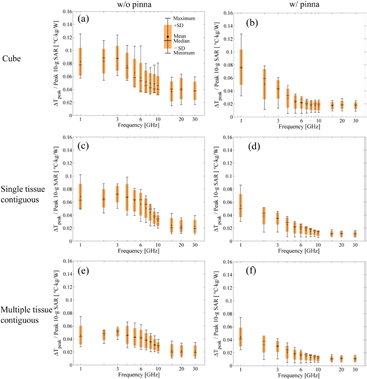
Figure 10 shows the heating factor in the brain of the different head models. Note that the peak 10 g-averaged SAR was calculated using averaging algorithms (I) and (IV). The same scenarios as in figure 4 were considered; the SAR and temperature elevation in five head models were computed for the dipole antenna located at the reference position and oriented in the up–down and front–back directions; 10 scenarios were considered for each frequency.
Figure 10. Variability of the heating factors in the brain of different human head models in the case of averaging algorithms (a) (I), (b) (II), (c) (III), (d) (IV), (e) (V), and (f) (VI). The antenna feeding position is the black circle in figure 1 and two polarizations are considered. The minimum, median, mean, and maximum values and the standard deviation of the heating factors are plotted.
Download figure:
Standard image High-resolution image
As shown in figure 10, the brain temperature reduced with an increase in the frequency, which is attributable to the decrease in the penetration depth of the electromagnetic fields. However, the brain temperature did not converge to zero, because the heat generated around the surface may diffuse up to a few centimetres into the head. A similar tendency was also observed for the other averaging algorithms, but to avoid repetition, these results are not shown here.
4. Discussion and concluding remarks
The heating factors obtained using different SARs as calculated using different averaging algorithms showed different frequency dependences and values. All the three factors considered as not being harmonised in the current standards and guidelines (ICNIRP 1998, IEEE-C95.1 2006), i.e. the number of tissues, averaging shape, and consideration of the pinna, are not negligible when discussing the appropriate averaging scheme to correlate the temperature elevation.
When the pinna is included in the SAR computation (averaging algorithms (II), (IV), and (VI)), the peak SAR value becomes large (see figure 3). However, the heating factor does not always become large, because the temperature elevation in the pinna also becomes large. When the SAR in the pinna is not considered, the heating factor (averaging algorithms (I), (III), and (V)) increases at higher frequencies. The SAR in the pinna contributes to the elevation of the temperature elsewhere in the head owing to heat conduction. Specifically, in TARO, the ratio of the power absorption in the pinna to that in the entire head is 10% at 1 GHz, 28% at 2 GHz, and more than 50% at frequencies higher than 5 GHz. The amount of power absorbed in the pinna is significantly affected by the shape of the pinna and its surrounding structure and anatomy (see figure S1).
The variability in the heating factors calculated with six averaging algorithms is investigated for the two main factors for a total of 300 exposure scenarios. From our computational results, the CVs obtained from the SAR averaging algorithms where the averaging shape is a cube are smaller than those for an arbitrary shape. For an arbitrary shape of the SAR averaging volume, CVs become large at frequencies higher than 10 GHz.
The strong correlation between the peak 10 g-averaged SAR calculated with algorithms (I) and (V) and the temperature elevation was observed for frequencies up to 3 GHz, as reported in previous studies (Hirata et al 2006a, McIntosh and Anderson 2010), supporting the description in the IEEE standard (2006). A modest correlation was observed when a frequency range of up to 10 GHz was considered for averaging algorithms (I) and (V). When considering the pinna, algorithm (VI) provided a better correlation with the temperature elevation than algorithm (IV), suggesting that multiple tissues would be better suited rather than a single tissue in the SAR averaging region. The values of R2 obtained when calculating the SAR with algorithms (III) and (V) for frequencies from 1 to 30 GHz were better than those for frequencies from 1 to 10 GHz. These results may be coincidental, but they are not surprising because the mean and median values of the heating factor calculated with algorithms (III) and (V) are frequency-insensitive. For any averaging scheme, conservative estimates for the temperature elevation could be obtained by multiplying the 95th percentile value of heating factor by the limit of the SAR.
An additional point to be stressed is that the heating factor in the head models changes gradually around the border frequencies (3 and 10 GHz), unlike the allowable output power from an antenna array derived from current guidelines and standards, which drops by an order of magnitude at the border frequency (Colombi et al 2015). Discussion on whether the incident power density or the peak spatial-averaged SAR is a better metric to correlate with the peak temperature elevation remains a topic for further research. Note that SAR measurement methods above 6 GHz is outside of the scope of this study.
As easily expected, the heating factor in the brain decreases with an increase in the frequency. The heating factor, however, does not decrease exponentially at higher frequencies, because of the heat conduction from the surface of the human head.
The main purpose of this study was to discuss the applicability of the peak spatial averaged SAR as the metric for the temperature elevation in the international safety guidelines/standards. Thus, the uncertainty and variability for product safety testing (e.g. different mobile phones) have not been discussed in this study; these issues are mainly discussed in International Electrotechnical Commission and IEEE ICES Technical Committee 34. Investigation on the uncertainty and variability is needed for the product safety when more detailed specification of wireless devices are clarified (see e.g. Hadjem et al 2005, Gosselin et al 2011, and Adibzadeh et al 2015a for frequencies lower than 3 GHz). Note that the metric used here is the ratio of the temperature elevation to the SAR, which is insensitive to antenna types and pinna conditions at least for frequencies lower than 3 GHz (Hirata and Shiozawa 2003), although the SAR varies to such factors.
In conclusion, when correlating the peak temperature elevation and the peak SAR, the averaging algorithms are the key factors. The SAR averaging algorithms excluding the pinna are essential to estimate the peak temperature elevation in the head excluding the pinna. In addition, allowing multiple tissues in the SAR averaging volume provided a better correlation than restricting the averaging volume to single tissue. For frequencies up to 3–4 GHz, strong correlations between the SAR and temperature elevation were obtained for different algorithms, whereas the correlations were at most modest at higher frequencies. The 95th percentile value of the heating factor and the mean and median values provide a conservative estimation of the peak temperature elevation for different frequencies and SAR averaging algorithms. The heating factors presented in this study may not be applicable for the temperature elevation higher than 1 °C (see section 2.3), because vasodilation have been suggested to cool down the temperatuure elevation even for localized exposure (Alekseev et al 2005).
Acknowledgment
This study was partly supported by the Ministry of Internal Affairs and Communications.